Geometric Targets for UAS Lidar

Abstract

Lidar from small unoccupied aerial systems (UAS) is a viable method for collecting geospatial data associated with a wide variety of applications. Point clouds from UAS lidar require a means for accuracy assessment, calibration, and adjustment. In order to carry out these procedures, specific locations within the point cloud must be precisely found. To do this, artificial targets may be used for rural settings, or anywhere there is a lack of identifiable and measurable features in the scene. This paper presents the design of lidar targets for precise location based on geometric structure. The targets and associated mensuration algorithm were tested in two scenarios to investigate their performance under different point densities, and different levels of algorithmic rigor. The results show that the targets can be accurately located within point clouds from typical scanning parameters to <2 cm $\sigma ,$ and that including observation weights in the algorithm based on propagated point position uncertainty leads to more accurate results.

1. Introduction

Airborne lidar, or laser scanning, from small unoccupied aerial systems (UAS) has gained a reputation as a viable mapping tool for both academic researchers and commercial users within the past decade (e.g., [1,2,3]). Accompanying the release of the lightweight Velodyne VLP-16 in 2014 was the emergence of highly-accurate, lightweight navigational hardware, eliminating the need for auxiliary sensor data, such as computer vision techniques used in the earliest UAS lidar studies [4]. These two core components form a payload that is functionally similar to the conventional airborne lidar payloads aboard piloted aircraft, but at a fraction of the weight and cost. Commercial outfits (e.g., LiDARUSA, YellowScan, Phoenix LiDAR Systems) have offered turnkey UAS lidar systems which utilize the VLP-16 since at least 2015 [2]. From an accessible platform, the UAS, users can now collect an established and familiar data product, the lidar point cloud, which is compatible with existing data processing workflows and analysis.

As with all geospatial data, it is important to characterize the spatial accuracy of lidar products to inform their appropriate use. Similarly, a measure of accuracy is important for rigorously adjusting lidar data, correcting for systematic errors, and fusing it with other geospatial datasets, such as photography [5]. Accuracy assessment of geospatial data typically involves the use of check-points, independently surveyed targets, or features within the captured scene, to produce statistical measures of accuracy often reported using the root mean square error (RMSE). However, comparison of lidar point clouds relative to check points can be problematic since individual lidar points are never exactly coincident with surveyed reference points. Often, only the elevation errors of points or derived raster digital elevation model (DEM) cells in the neighborhood of a reference surface are used, neglecting any measure of horizontal errors. This is the case for both conventional occupied-platform lidar and UAS lidar [6].

Historically, the development of accuracy assessment methods for lidar was limited due to the relatively sparse spatial density of the points [7]. Continual advancements in technology have led to rapidly-increasing point densities, with contemporary large systems capable of collecting over 1 million point measurements per second, thus allowing for the use of artificial targets for full 3D accuracy assessment of the data. Targets designed to intercept several points enable a more holistic assessment of the positional accuracy of point clouds and are more appropriate for characterizing accuracy for applications that involve using several points to reconstruct and measure features, such as the synthesizing and measurement of buildings, roadway structures, and tree morphology models.

Hardware calibration is a critical component of processing lidar data and consists of estimating systematic parameter errors associated with the physical alignment of sensor mechanisms [8]. These include the lever arm and boresight parameters: the location and angular orientation, respectively, of the scanner head relative to the navigation reference point of the system, usually the inertial measurement unit (IMU). In addition to these, other parameters are often captured in the calibration procedure associated with, for example, biases in the laser scanning mechanism.

Like calibration, lidar strip adjustment is used to bring collection units, swaths associated with flight lines, into alignment. The adjustment is often generic [9]. That is, it does not attempt to model actual physical parameters due to the inaccessibility of requisite data, such as vehicle trajectories. The effects of errors in physical calibration parameters as well as errors not modeled in calibration, e.g., biases in trajectory due to navigation solution drift, may be absorbed into the geometric transformation parameters.

Both calibration and strip adjustment algorithms often use the identification of points associated with geometric primitives, such as planes or lines in the scene, to detect discrepancies between overlapping collection units to be used as observations in optimization schemes for resolving the parameters. However, many scenes do not have planar surfaces or features composed of these primitives, or the features are not distributed in an optimal geometric configuration to best resolve the parameters. Some algorithms avoid the use of primitives by using the points themselves, diminishing structural requirements on the scene. These include iterative closest point (ICP) and iterative closest plane variants [10]. These methods can be time-consuming, and require close initial approximations. Furthermore, some scenes are dynamic and complex, such as forests in windy conditions, and the fundamental assumption that features or points are in the same place from collection unit to collection unit is violated. Effects are amplified for smaller mapping regions and higher point densities associated with UAS lidar. They can be mitigated by using large portions or all of the point cloud in the adjustment, but at the cost of processing time. Artificial lidar targets may provide a way to address these issues associated with calibration and strip adjustment.

Past studies on lidar targets employed a variety of different approaches. The study presented in [11] used circular targets with a bright white center on a dark black background to exploit point intensity data in determining which points fell within the central circle. A method similar to the generalized Hough-transform circle-finding method was used to find the horizontal location of the circle within the point cloud, and the average point height was used to estimate the vertical component. The estimated positioning accuracy of the elevated 2 m diameter targets was around 5–10 cm and 2–3 cm for the horizontal and vertical components, respectively, at a lidar point density of 5 pts/m². The study in [12] used white L-shaped targets painted on asphalt to similarly locate 3D positions within lidar-derived intensity images using least-squares matching [13]. The study in [14] used retro-reflective targets in a hexagonal configuration to find a location within a relatively sparse point cloud (approximately 2 pts/m²) to aid in boresight calibration, with reported location precision of 5 cm and 4 cm in the vertical and horizontal components, respectively. The dimensions of a proposed, but not yet implemented, foldable 3D target were illustrated by [15], designed to use solely the point positions, and not intensity.

The current applied methods for targets in UAS lidar primarily employ bright flat targets which make use of the intensity value of lidar returns available in most scanners. For example, [16] used ICP to align UAS lidar swaths, ground control points (GCPs) marked with flat sheet targets to apply an absolute correction, and targeted and untargeted ground-surveyed checkpoints for accuracy analysis. The method in [17] used the average location of points striking reflective ground targets for accuracy assessment. That study described critical issues with this approach, including assumed distribution of points striking the target and effects of the laser beam divergence leading to bias and/or lower accuracy of measured locations in the point cloud compared to expectations from stochastic modeling. Similarly, [17] used reflective ground targets manually measured in UAS point clouds, but details of the method were not described. There is not much exploration of mensuration uncertainty, the uncertainty of target location within the point cloud, in the literature, and thus a direct comparison of the various targeting methods is not possible.

Often, the use of intensity is not a robust solution for artificial targeting in laser scanner data. For example, the Velodyne VLP-16 is one of the most commonly-used UAS laser scanning systems. As reported by [18] and in the present authors’ experience, the VLP-16 intensity reading quality is highly dependent on range and the incidence angle of the beam with the intercepting object. Additionally, intensity is recorded at a lower quantization level than larger and more-expensive laser scanners [19]. At the low altitudes associated with UAS platforms, incidence angles for small homogenous areas and objects in the scene can have very diverse incidence angles, and therefore objects with similar reflectivity can yield substantially diverse intensity readings when surveyed in the typical boustrophedonic overlapping-swath flight pattern. It is often difficult, for example, to locate points from overlapping swaths associated with a white paper plate on healthy grass based on intensity from the VLP-16 as illustrated in Materials and Methods section. Use of very bright objects may be one approach to addressing this issue. However, [18] indicates that high-intensity VLP-16 readings are associated with range bias on the order of a centimeter, which has also been observed by the present authors. In addition to issues associated with locating target points by intensity, the flatness of targets can also be problematic. As [4] mentioned, non-uniform point distribution on the target can lead to poor, biased resolution of the horizontal reference point of the target, often located in the center of extreme target points, e.g., x = (max_x − min_x)/2. This is the case for both automatic methods and manual methods, where an operator estimates the center location of the target and interpolates the elevation of the target center based on surrounding points. To address these issues, this study introduces an alternative to intensity-based artificial targets for UAS lidar. More specifically, this study presents:

• The description of a developed small-UAS laser scanning system;
• The design of geometric structure-based targets which can be used for accuracy assessment, calibration, and strip adjustment;
• Mensuration algorithms for precise target location within point clouds;
• Two case studies illustrating the efficacy of the targets and associated algorithms for accuracy assessment.

While the accuracy results of the UAS system are presented and are of interest, they are not the focus of the paper. Instead, we focus on the methods to achieve the accuracy assessment, which can be used for other similar UAS laser scanning systems. It should be noted that UAS lidar accuracy may vary depending on site location, control configuration and accuracy, system characteristics, and mission planning.

2. Materials and Methods

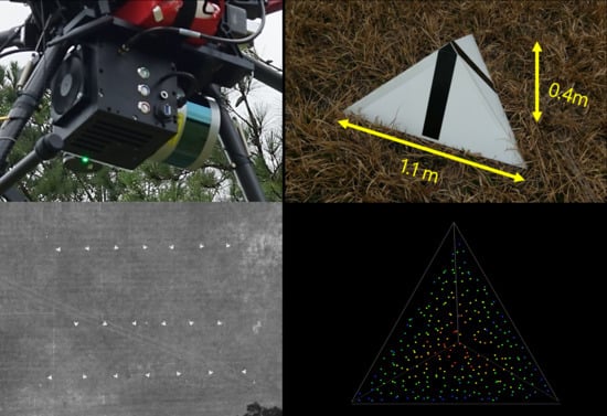
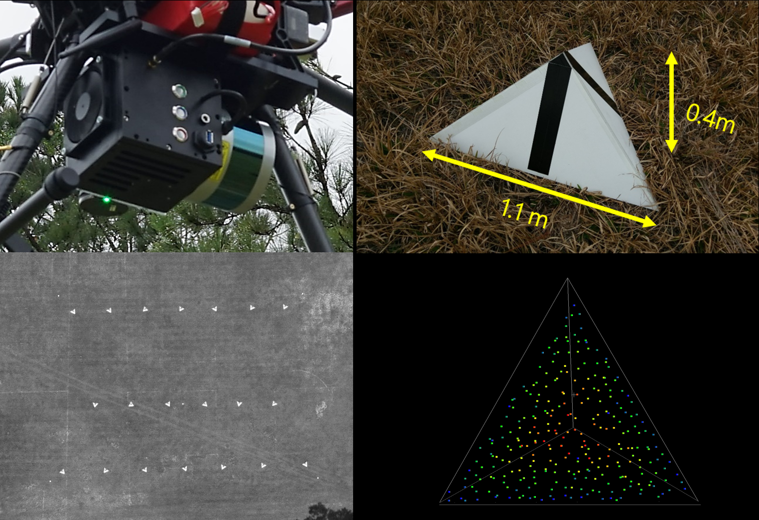
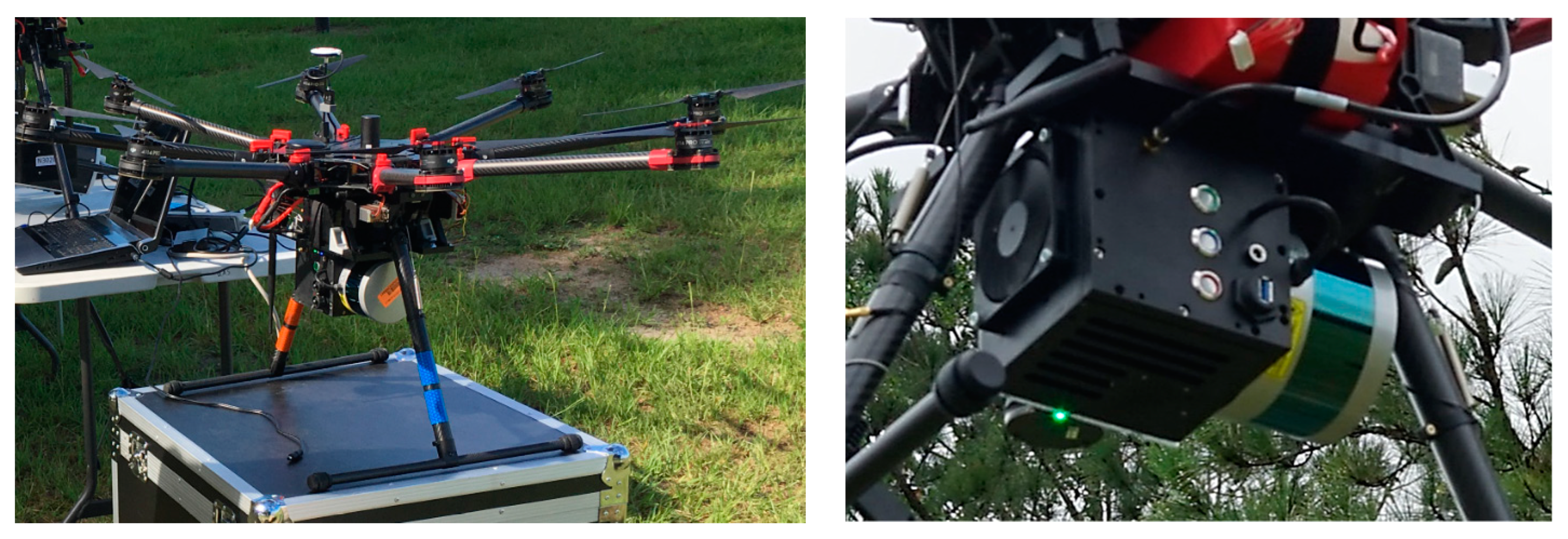
The UAS laser scanning system used in this study (Figure 1) comprised a DJI s1000 octocopter with a sensor payload consisting of a Velodyne VLP-16 Puck Lite laser scanner head, NovAtel OEM615 Global Navigation Satellite System (GNSS) receiver, STIM300 IMU, Garmin GPS18x—for time stamping outgoing lidar pulses, a NovAtel GPS-702-GG antenna (Experiment Site 1 only), and a Maxtena M1227HCT-A2-SMA antenna (Experiment Site 2 only). Although this system was designed and built by our team, it can be considered typical, with various commercially-available turnkey analogues. Similarly, processing algorithms to generate point clouds from raw laser scanner and navigation sensor data, calibrate the sensor, and perform strip adjustment were developed internally. They can also be considered standard, except that they were designed to use our developed targets, and had the capability to propagate and carry forward uncertainties from the navigation and scanner observations to the point cloud. This allowed the estimated standard deviations of the X, Y, and Z components of each point in the point cloud to be stored and accessed, a benefit that we explored in our target mensuration experiments.

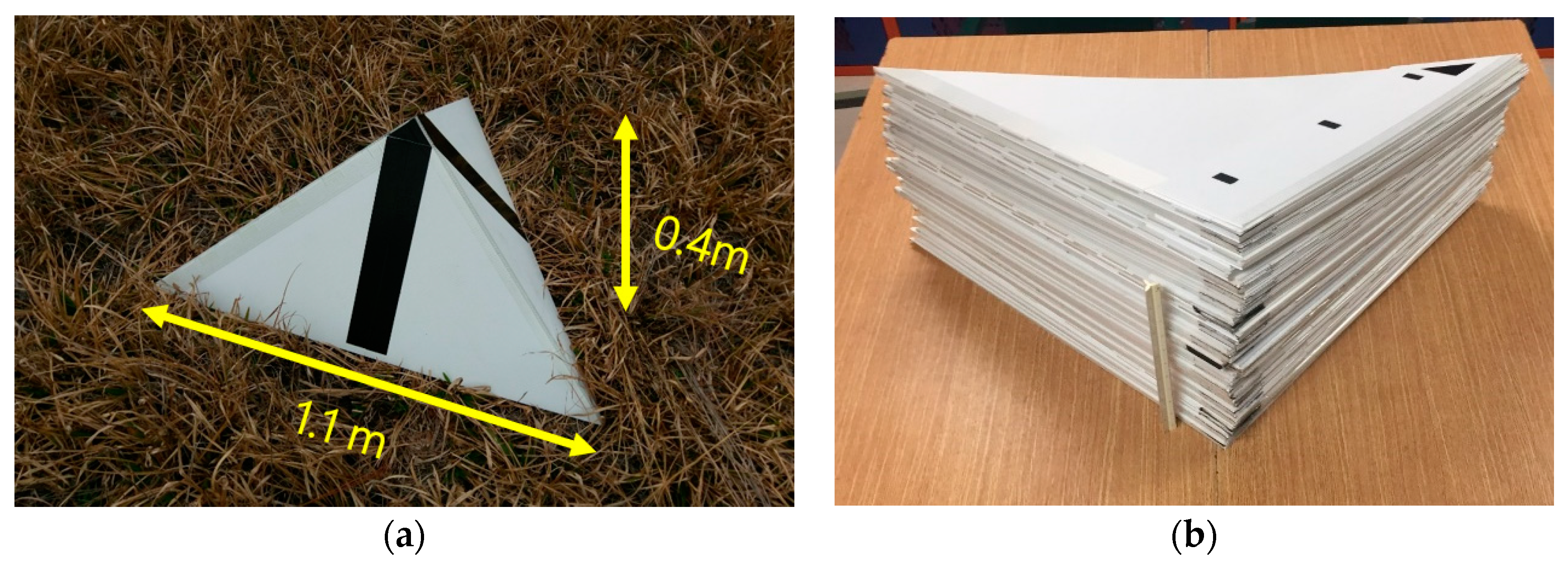
A primary objective of this study was to create portable, inexpensive, and multimodal (measurable in both lidar point clouds and imagery) targets capable of establishing accurate 3D locations within a point cloud from associated point observations with practical densities and distributions associated with UAS–lidar systems. The resulting design is shown in Figure 2. The targets were foldable, corner-cube trilateral pyramids made from white corrugated plastic. The base of the pyramid was 1.1 m and the peak was 0.4 m above the ground when deployed. The reference location, to where ground-survey and point cloud coordinates were measured, was where the three planes intersected at the peak. The targets’ foldability allowed for easy transport and storage. Figure 2b shows a stack of 22 targets, which could be easily carried by a single person. Black tape was placed on the pyramids to allow for measurement of the reference point, the intersection of the centerline of the three black lines, in photography taken from any perspective showing at least two sides of the target.

The mensuration algorithm for locating targets in the lidar point cloud was an iterative least-squares process to fit a known target template, three intersecting planes based on the design dimensions of the target, to points associated with it using rigid-body six-parameter transformation (3D rotation followed by translation) [20]. The template’s untransformed coordinate system origin was located at the reference point at the tip of the pyramid, the base was parallel with the horizontal plane (close to what will likely be the fitted pose, hastening convergence), and one of the edges was aligned such that y = 0 (Figure 3). This edge orientation was arbitrarily chosen, with any orientation leading to convergence of the mensuration algorithm, meaning that actual targets need not be aligned with any particular orientation when placed in the field.

The first step was to identify and isolate points associated with the target. In this study, segmentation of target points was done manually, based on the relative height of the points above the ground. Automatic extraction of these points was feasible by using a random sample consensus (RANSAC) [21] variant of the mensuration algorithm, which is proposed for future work. Nevertheless, manual segmentation was straightforward due to the structure of the targets. Figure 4 and Figure 5 illustrate the identifiability of target points based on height compared to that based on intensity. The mensuration algorithm presented here allowed the use of any subset of the points on the target, as long as some points on each facet were found. The distribution of the points did not bias the estimated target location, a quality that is explored in the Appendix A. This allowed the user to be conservative in the confident identification of target points, reducing the possibility of blundered selection of non-target points.

The target transformation parameters were initialized by setting the orientation angles equal to zero: $\omega =0$, $\phi =0$, and $\kappa =0$, where $\omega$, $\phi ,$. $\kappa$ are sequential rotations about the target $X, Y$, and $Z$ axes, respectively. Translation $\mathit{T}={\left(T_X, T_Y, T_Z\right)}^{\mathrm{T}}$ was initialized to be equal to the coordinates of the highest of the target points.

Each iteration of the least-squares solution begins with identifying the closest facet, $f_{\min }$, of the template in its current pose for each point. This is accomplished by finding the minimum dot product of the unit normal vectors of each facet $f$, ${\mathit{n}}_f={\left(n_{f,x},n_{f,y},n_{f,z}\right)}^{\mathrm{T}}$ with $\left({\mathit{x}}_p-\mathit{T}\right)$, where ${\mathit{x}}_p={\left(x_p,y_p,z_p\right)}^{\mathrm{T}}$ is the position of the point $p$. Jacobian matrix $\mathit{J}$. is formed (Equation (1), where $m$ is the number of points), containing the partial derivatives of the distance, $d_i$, of each point $i$ to its associated plane with respect to the six transformation parameters:

$$\mathit{J}=\left[\begin{array}{cccccc}\partial d_1/\partial \omega & \partial d_1/\partial \phi & \partial d_1/\partial \kappa & \partial d_1/\partial T_X& \partial d_1/\partial T_Y& \partial d_1/\partial T_Z\\ \partial d_2/\partial \omega & \partial d_2/\partial \phi & \partial d_2/\partial \kappa & \partial d_2/\partial T_X& \partial d_2/\partial T_Y& \partial d_2/\partial T_Z\\ ⁝& ⁝& ⁝& ⁝& ⁝& ⁝\\ \partial d_m/\partial \omega & \partial d_m/\partial \phi & \partial d_m/\partial \kappa & \partial d_m/\partial T_X& \partial d_m/\partial T_Y& \partial d_m/\partial T_Z\end{array}\right]$$

(1)

Finally, a vector containing the negatives of the point-to-plane distances is formed, $\mathit{\epsilon }=-\mathit{d},$ enabling the least-squares solution to the linearized observation equations using Equation (2):

$$\Delta ={\left({\mathit{J}}^{\mathrm{T}}\mathit{J}\right)}^{-1}{\mathit{J}}^{\mathrm{T}}\mathit{\epsilon }$$

(2)

In Equation (2), $\Delta$ contains corrections to the current approximations of the transformation parameters. The process is repeated until convergence of the standard deviation of unit weight, with the final resolved translation components, $\mathit{T},$ serving as the estimated position of the reference point.

If propagated uncertainties for point coordinates are available, the algorithm has the same steps, except that the solution is:

$$\Delta ={\left({\mathit{J}}^{\mathrm{T}}\mathit{W}\mathit{J}\right)}^{-1}{\mathit{J}}^{\mathrm{T}}\mathit{W}\mathit{\epsilon }$$

(3)

In Equation (3), $\mathit{W}={\left(\mathit{A}\mathbf{\Sigma }{\mathit{A}}^{\mathrm{T}}\right)}^{-1},$ where $\mathit{A}$ is the Jacobean matrix with rows containing the partial derivatives of the distances of each point, $d_p,$ to their associated planes with respect to ${\mathit{x}}_p$:

$$\frac{\delta d_p}{\delta {\mathit{x}}_p}={\mathit{n}}_{f_{\min }}$$

(4)

$\mathbf{\Sigma }$ is the covariance matrix associated with lidar point coordinate uncertainty. The effect of including this weighting in the mensuration algorithm was explored in the experiments for Site 2.

The covariance matrix of the target template transformation parameters, ${\mathbf{\Sigma }}_{\Delta \Delta }$, may be calculated using Equation (5). The elements of ${\mathbf{\Sigma }}_{\Delta \Delta }$. associated with the translation components, $T_X, T_Y, T_Z,$ can be used as estimates of the target mensuration uncertainty:

$${\mathbf{\Sigma }}_{\Delta \Delta }={\left({\mathit{J}}^{\mathrm{T}}\mathit{W}\mathit{J}\right)}^{-1}$$

(5)

Note that in this study, point position uncertainties were based on propagated variance from navigation parameters and scanner-head hardware. Inter-state correlations among these components were not resolved (i.e., the weight matrix associated with point-to-plane distances, $\mathit{W},$ was a diagonal matrix), and thus it was expected that propagated uncertainties of the target positions would be optimistic, since the assumed independence of point positions, and therefore point-to-plane distances, was violated. Obtaining estimates of the inter and intra-state correlation among navigation and scanner head parameters was not readily achieved, as they are not fully available in commercial navigation processing software and from scanner hardware vendors, respectively. Still, the outcomes from this study presented in the Results and Analysis section suggest that the propagated uncertainties used, even without accounting for correlation among parameters, were valuable.

Since lidar points near target edges may have convoluted echoes and lead to spurious observations, each point is tested for edge proximity. If a point is closer to an edge than a selected tolerance it is removed from the solution. In this study, points were culled if they were closer than one fourth of the beam diameter to an edge, a tolerance found empirically to improve the fidelity of the observations without overly decreasing redundancy. Similarly, points were removed if their orthogonal projection onto their associated facet-planes fell outside of the facet triangle. Points were tested in each iteration of the solution after the first two iterations were completed (the algorithm requires at least three iterations before convergence is established). The distance of a lidar point $p$ to a target edge $e_{i,j}$ associated with vertices ${\mathit{v}}_i$ and ${\mathit{v}}_j$, where ${\mathit{v}}_i={\left(x_{{\mathit{v}}_i},y_{{\mathit{v}}_i},z_{{\mathit{v}}_i}\right)}^{\mathrm{T}}$, is:

$${\mathit{d}}_{p, e_{i,j}}=\frac{\Vert \left({\mathit{x}}_p-{\mathit{v}}_i\right)\times \left({\mathit{x}}_p-{\mathit{v}}_j\right)\Vert }{\Vert {\mathit{v}}_i-{\mathit{v}}_j\Vert }$$

(6)

The projection of a point $p$ onto the plane containing target vertices ${\mathit{v}}_i$, ${\mathit{v}}_j,$ and ${\mathit{v}}_k$. associated with the closest target facet $f_{\min }$ is:

$${\mathit{x}}_p^{\prime }={\mathit{x}}_p-{\mathit{n}}_{f_{\min }}\left({\mathit{n}}_{f_{\min }}·\left({\mathit{x}}_p-{\mathit{v}}_i\right)\right)$$

(7)

If ${\mathit{x}}_p^{\prime }$ is inside of the triangle formed by ${\mathit{v}}_i$, ${\mathit{v}}_j,$ and ${\mathit{v}}_k$, the barycentric coordinates of ${\mathit{x}}_p^{\prime }$ with respect to the triangle will all be positive. This condition is used to test if the orthogonal projections of points fall on their associated target facets.

Two separate study areas were used to illustrate the efficacy of the pyramidal target methods. The first (Site 1) was used to illustrate precision and how lidar point density affects target mensuration within the point cloud, and the other (Site 2) to illustrate the benefit of using error propagation to locate targets.

Site 1 was located in Jonesville, Florida, at a recreation/sports park. Site 2 was located within Ordway Swisher Biological Station (OSBS), a 9500-acre University of Florida research facility in Melrose, Florida, which is primarily used for ecosystem monitoring and management research. The planned mission parameters are shown in

Table 1. Mission parameters for the accuracy test flights.

	Flight Lines			Combined Point Cloud
Site	# Flight Lines	Length/Spacing	Repetitions	Density *	Spacing
Site 1: Jonesville	3 North-South	70 m/25 m	2 at 40 m AGL 1 at 30 m AGL	3000 pts/m2	1.8 cm
Site 2: OSBS	3 North South	200 m/25 m	1 at 30 m AGL	800 pts/m2	3.5 cm

* Single-swath point density is essentially the same for 30 m flying height at both sites.

.

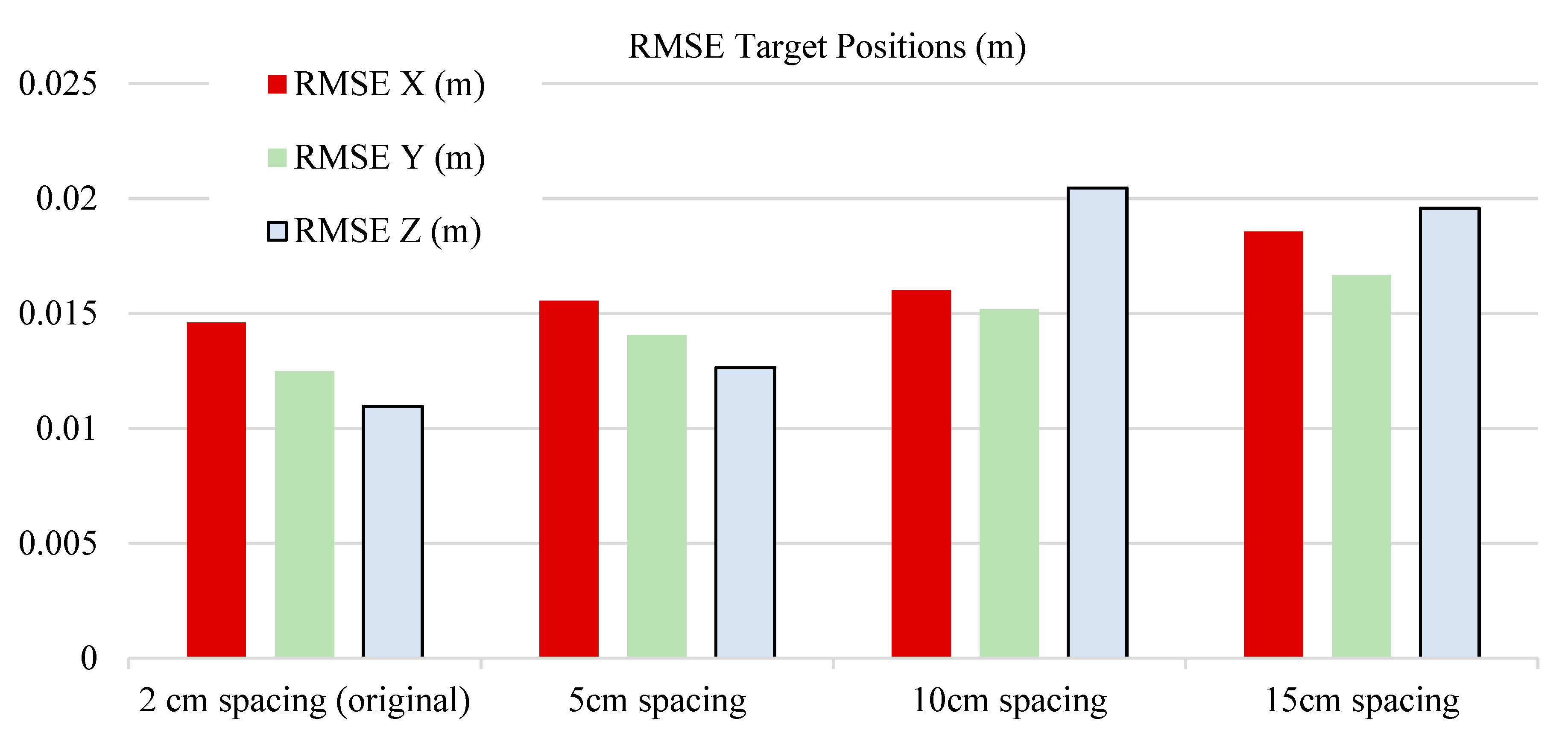
Site 1 consisted of three north-to-south flight paths (Figure 6). Data were collected along these flight paths and associated turns twice at 40 m and once at 30 m flying height above ground level (AGL). The area was scanned with the full outgoing pulse rate of the VLP-16, 300 kHz, yielding an average combined-swath pulse density of 3000 pts/m², or an approximate point spacing of 1.8 cm in the center of the project area. The scan rate was 10 Hz, although it should be noted that later investigation found maximizing the scan rate of the VLP-16 yielded better point distribution, reducing clustering of points, albeit with lowered point accuracy due to lower resolution of the encoded scan angles. In order to investigate the effect of point density on target mensuration, the original processed point cloud was decimated three times to generate target point clouds with 5 cm, 10 cm, and 15 cm minimum 3D point distances, by iteratively and randomly selecting points and removing all neighbors within less than the minimum 3D point distance. Initially, 20 cm point spacing was also attempted, but it sometimes (2 of 20 targets) led to failure of the target mensuration algorithm and was excluded from analysis.

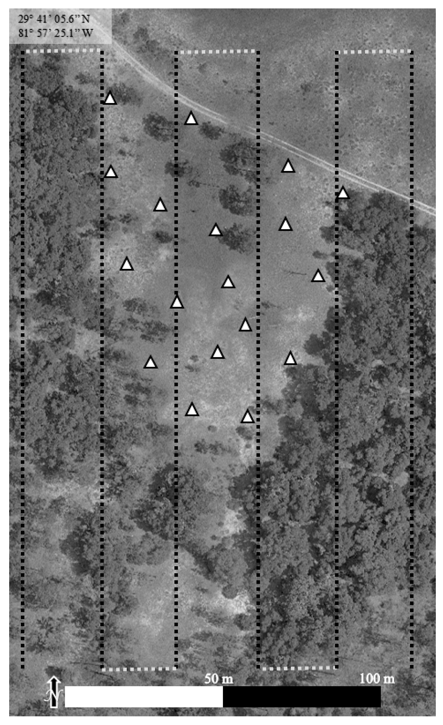
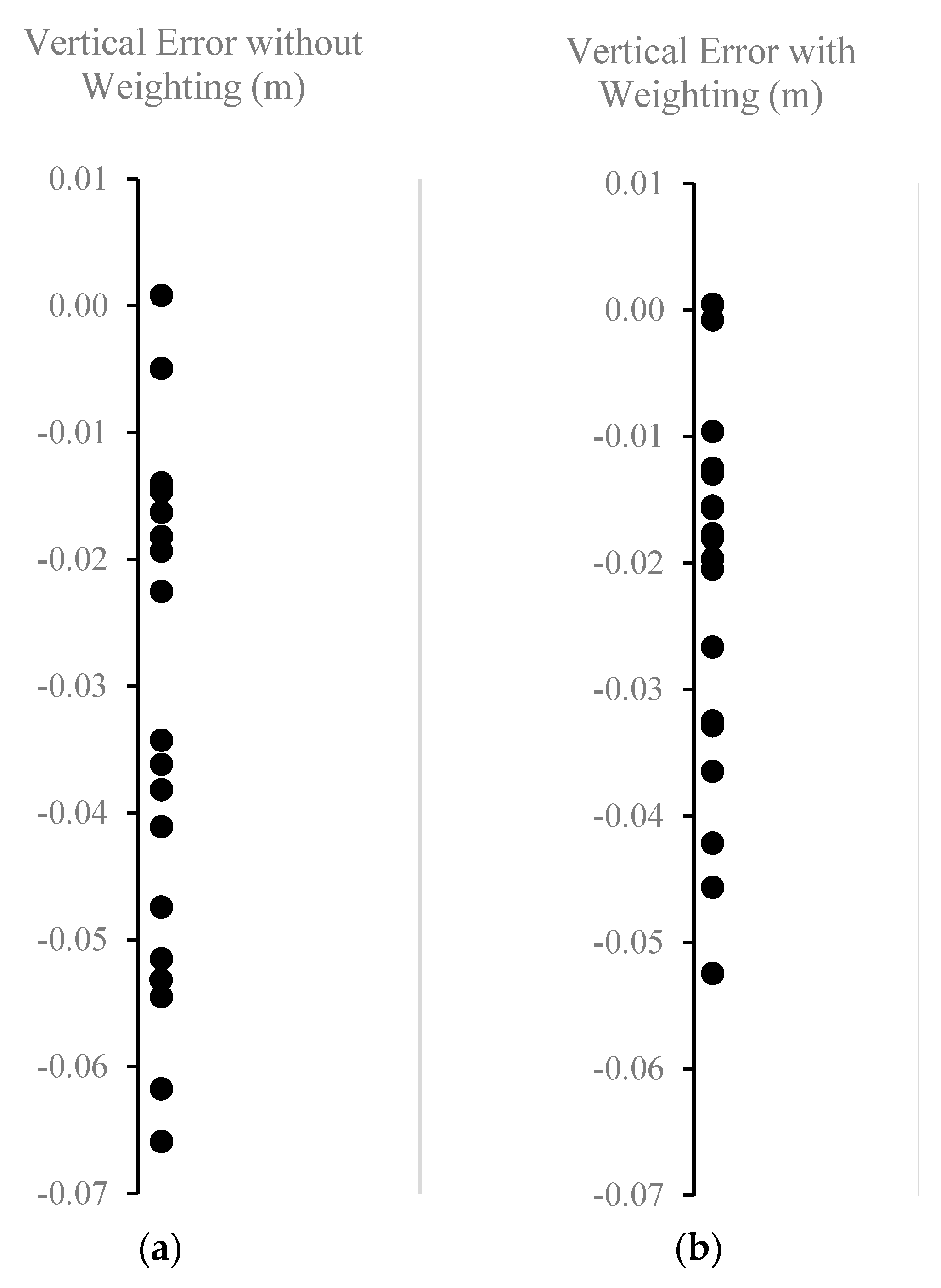
Site 2 data were collected via a single repetition of six flight lines stretching 200 m north-to-south, and with 25 m line separation (Figure 7). The area was scanned at 30 m flying height above ground, with a pulse rate of 300 kHz, and 10 Hz scan rate. The average combined point cloud pulse density was approximately 800 pts/m², or a point spacing of approximately 3.5 cm. Note that since the Site 2 flight paths were longer, the increase in the average point density associated with points collected on turns between primary lines was smaller than that for Site 1. Similarly, the longer lines for this flight led to higher uncertainty for some target-associated points, since uncertainty is largely dependent on laser range, making this dataset well-suited for the analysis of uncertainty-based weighting on target mensuration. To study this, the target locations were estimated using both the weighted and unweighted versions of the mensuration algorithm.

Boresight calibration of the laser scanner sensor suite, estimation of the angular alignment of the scanner head with respect to the platform axes corresponding to the filtered trajectory (IMU axes), was carried out for both missions, each time using three targets without using ground survey coordinate observations. The details of the boresight procedure are beyond the scope of this paper, but details will be given in a future article. Strip adjustment, alignment of the overlapping swaths, was not necessary to bring collection units into alignment for this study, since there was no observable discrepancy between flight strips after the boresight calibration procedure.

At each site, the targets were used to mark ground-surveyed checkpoints, which were well-distributed across the project area. There were 20 checkpoints within Site 1 that were nominally spaced at 7 m along three north–south rows. The eastern-most row was approximately 14 m from the central row, and the western-most row was 20 m from the central row. These can be seen in Figure 6. Site 1 target coordinates were established using post-processed kinematic (PPK) GNSS. The rover GNSS antenna was held above the targets so that the processed coordinates could be reduced to the target reference points. It is important to mention that the target survey used the same base station that was used to calculate the UAS trajectory, albeit at different times, and thus the two were not entirely independent. Site 2 had 18 widely distributed checkpoints, with a mean nearest neighbor distance of 22 m. Figure 7 shows the distribution of Site 2 targets. Site 2 target coordinates were established using a total station, with distances corrected for map projection distance scale. A reflective surveying prism was held above the targets so coordinates could be reduced to the target reference points. Similar to Site 1, since total station back sight observations were made to a (non-lidar-targeted) point with coordinates established by the same GNSS observations that were used for calculating the UAS trajectory, target coordinates were not completely independent from the estimated UAS trajectory.

3. Results and Analysis

3.1. Site 1: Target Point Precision and Accuracy, and Effect of Point Density

The extremely high point density of Site 1 allowed an analysis of the impact of point density on target point accuracy. Since the study area had flat, level terrain, the tilt parameters of the target, $\omega$ and $\varphi$, were constrained to zero. If they are solved for in the mensuration routine, a systematic error is observed at low point cloud densities. This effect is described in more detail at the end of this sub-section. Example distributions of target points at different densities are shown in Figure 8. In the figure, note that the edges of the point clouds do not follow exactly the edges of the template, since they were manually segmented prior to mensuration without knowledge of the exact target location. This is entirely allowable with the mensuration algorithm, and enables aggressive segmentation to avoid the inclusion of non-target points. The average estimated target position mensuration uncertainties for various point densities, based on Equation (5), are given in

Table 2. Average estimated target mensuration uncertainty for various point spacings at Site 1.

Spacing.		Average Estimated Mensuration Uncertainty (m)
	Average Points Per Target	${\overline{\mathit{\sigma }}}_{\mathit{X}}$	${\overline{\mathit{\sigma }}}_{\mathit{Y}}$	${\overline{\mathit{\sigma }}}_{\mathit{Z}}$
2 cm	1141	0.002	0.002	0.002
5 cm	183	0.005	0.005	0.005
10 cm	41	0.010	0.010	0.010
15 cm	18	0.015	0.015	0.015

. Note that based on the average number of points per target (given in Table 2), the standard deviations relative to each other could be approximated by ${\overline{\sigma }}_i\approx {\overline{\sigma }}_j\sqrt{n_j/n_i}$ where $n_i$ is the number of points on the target for spacing $i$, which is expected.

Mensuration uncertainty increased with an increase in point spacing, since fewer observations were included in the position estimates. The estimated standard deviations were 1 cm or less for each component for all point spacings less than 15 cm. All components had nearly identical mensuration uncertainty; however, it is important to note this was not the case when tilt angles were included as unknowns where the Z uncertainty was larger than that for the horizontal components. With a point spacing of 15 cm, the standard deviations were all 1.5 cm. This is near the upper-limit for practical application, approaching the level of independent GCP measurement uncertainty. Based on this estimate it is recommended that point spacing not exceed 10 cm for precise target mensuration.

The results for target position errors based on field-surveyed check-point coordinates are given in

Table 3. Accuracy assessment for various point spacings at Site 1.

Spacing	RMSE (m)			Mean Error (m)			Standard Deviation (m)
	RMSEX	RMSEY	RMSEZ	${\overline{\mathit{\epsilon }}}_{\mathbf{X}}$	${\overline{\mathit{\epsilon }}}_{\mathbf{Y}}$	${\overline{\mathit{\epsilon }}}_{\mathbf{Z}}$	${\mathit{\sigma }}_{\mathit{X}}$	${\mathit{\sigma }}_{\mathit{Y}}$	${\mathit{\sigma }}_{\mathit{Z}}$
2 cm	0.015	0.012	0.011	0.013	0.001	0.005	0.008	0.013	0.010
5 cm	0.016	0.014	0.013	0.013	−0.001	−0.005	0.009	0.014	0.012
10 cm	0.016	0.015	0.021	0.013	−0.002	−0.013	0.010	0.015	0.016
15 cm	0.019	0.017	0.020	0.012	0.002	−0.013	0.015	0.017	0.015

and illustrated in Figure 9. The errors were not distributed significantly differently from a normal distribution based on the Shapiro–Wilk test for normality (p > 0.05). The results show that RMSE values increased with point spacing, and generally followed the trend of estimated mensuration uncertainty. There was not enough information to make a statistically-rigorous statement about the power of estimated mensuration uncertainty to predict target accuracy, but the results are consistent in this study. The RMSE increased with estimated mensuration uncertainty, and thus it could be considered an effective way to predict the expected accuracy of target locations within point clouds at various point densities. Mensuration uncertainty values were lower than the RMSE values, as expected due to imperfections in point location uncertainty estimation methods, as discussed in the Methods section, and due to errors in the surveyed coordinates of the check points not accounted for by mensuration uncertainty. The difference between mean square error and estimated mensuration variance was in the order of the expected field-surveyed coordinate mean squared error, approximately 1 to 2 ${\mathrm{cm}}^2$.

Significant differences could not be found for the mean errors of the horizontal components based on t-tests of difference of means. The mean error in the vertical component for the 2 cm point spacing was found to be significantly different than all other point spacings (p < 0.01). The mean vertical error for the 5 cm point spacing was not significantly different to that for the 10 cm and 15 cm point spacings (p = 0.08 and p = 0.07, respectively), and the mean vertical error for the 10 cm point spacing was not significantly different to that for the 15 cm point spacing (p = 0.97). Coordinate error standard deviations always increased with point spacing. A significant difference was found between the X component variance of the 15 cm spacing coordinates and that from the 2 cm and 5 cm point spacing (p < 0.003, p < 0.02, respectively). The Z component variance was found to be significantly different for the 2 cm spacing compared to the 15 cm spacing (p < 0.05).

Based on these results, the developed targets provide a means to identify precise locations within UAS-lidar point clouds, and therefore are appropriate for accuracy assessment and use as conjugate features in data adjustment. For targets with the dimensions used in this study, it is recommended that average point spacing be around 5 cm and ensured to be less than 10 cm to obtain accurate within-cloud mensuration relative to check-point accuracy. This is readily achievable in practice with common scanners, such as the VLP-16, and UAS lidar products are often within this tolerance. However, it is expected that larger targets would allow for wider point spacing. The predicted uncertainty in target mensuration agreed with check-point accuracy results, and can be used in determining appropriate use of the targets, and guide mission planning to ensure adequate practical mensuration precision. As mentioned in the Materials and Methods section, 20 cm spacing led to failure of the mensuration algorithm with gross errors in 2 of the 20 targets. Removal of these two targets yielded RMSE values of 0.024 cm, 0.022 cm, and 0.044 cm for X, Y, and Z components for 20 cm spacing. Although these values may be acceptable for some applications, we did not include them in the analysis, since the algorithm had a high likelihood of failure.

It should be noted that results from initial experiments when including all three angular parameters as unknowns in the mensuration algorithm showed that when the point density decreased, the estimated centroids of the target templates fitted to the points tended to remain similar, but the angular orientations of the estimated target poses had substantially increased error, particularly for 15 cm spacing. Error in tilt of the target about the centroid of the points displaces all components, X, Y, and Z, of the reference point of the target (top of the pyramid). The Z component of the reference point is always shifted down with increased random tilt error about the centroid of the target, leading to a negative vertical bias increasing in magnitude as tilt error increases with point spacing. To allow for a fair comparison of higher point spacings in the experiments, the tilt parameters were constrained to zero for all trials at Site 1. This was viable since the ground was flat and level at the site. In practice, leveling the targets is achievable on moderately sloped ground.

3.2. Site 2: Effect of Uncertainty Estimation and Proper Weighting on Target Point Accuracy

All of the target coordinates for Site 1 were found using least squares with a weighting scheme based on the propagated uncertainty of point coordinates, as shown in Equation (3). Due to the larger area of Site 2, more points were associated with longer scanner ranges. Thus, points had larger average uncertainty, and a wider range of target point location errors and associated propagated uncertainties. This enabled an opportunity to compare the effects of including uncertainties in weighting the mensuration algorithm. The results of using the weighted and non-weighted schemes for Site 2, as presented in the Methods section, are shown in

Table 4. Position error statistics based on ground-surveyed target coordinates at Site 2 for weighted and unweighted mensuration methods.

Solution Method	RMSE (m)			Mean Error (m)			Standard Deviation (m)
	RMSEX	RMSEY	RMSEZ	${\overline{\mathit{\epsilon }}}_{\mathbf{X}}$	${\overline{\mathit{\epsilon }}}_{\mathbf{Y}}$	${\overline{\mathit{\epsilon }}}_{\mathbf{Z}}$	${\mathit{\sigma }}_{\mathit{X}}$	${\mathit{\sigma }}_{\mathit{Y}}$	${\mathit{\sigma }}_{\mathit{Z}}$
Unweighted	0.036	0.040	0.038	−0.012	0.034	−0.033	0.035	0.022	0.020
Weighted	0.028	0.034	0.027	−0.013	0.029	−0.023	0.026	0.018	0.015

and Figure 10 and Figure 11. The target coordinate errors were not distributed significantly differently from a normal distribution based on the Shapiro–Wilk test for normality (p > 0.05).

Using the weighted method yielded lower RMSE values for each of the X, Y, and Z components of the estimated target reference point. Mean errors magnitudes (with the exception of the $\mathrm{X}$ component) and standard deviations of target point errors were also lower when using the weighted method. These results suggest it is advantageous to use the weighted scheme when measuring the target points and any other derived multi-point feature within the point cloud, such as corners or planar surfaces. Substantial statistical significance could not be established for the difference in variance for any components X (p = 0.12), Y (p = 0.17), Z (p = 0.11), and the mean errors were also not found to be significantly different for X (p = 0.96), Y (p = 0.47), and Z (p = 0.10).

In addition to the apparent increase in precision and accuracy from using the weighted algorithm, inspection of the normalized residuals from each solution indicated that observation errors were better modeled using the weighting scheme. Figure 12 shows histograms of all normalized residuals for all the weighted and unweighted solutions.

As specified in the Methods section, the residuals are the distances, $\mathit{d},$ of the points to their associated target facets after solution convergence. The unweighted residual distribution had kurtosis of 3.39 (standard error (SE) = 0.06) and skewness of 0.96 (SE = 0.03). The weighted residuals had kurtosis of 1.68 (SE 0.06) and skew of 0.42 (SE 0.03). Weighted observations led to more normally distributed residuals and ignoring observation uncertainty led to higher kurtosis and skew. Higher kurtosis indicates heavy-tailed distributions and observations presenting as potential outliers relative to the expected normal distribution of their errors. While removing points with high residuals will decrease the kurtosis and potentially improve the solution, a better approach is to properly weight them to retain observation redundancy, as presented here.

4. Discussion

In Site 1, the estimated mensuration uncertainty and standard deviations of ground-surveyed checkpoints were less than 2 cm for point spacings up to 15 cm in all components, X, Y, and Z. To guarantee mensuration within the expected error of ground-surveyed points, it is recommended to not exceed 10 cm. Although the experiments indicated a significant decrease in mensuration accuracy in the sparsest clouds, the approach enabled target location and yielded reliable measured coordinates up to a spacing of 15 cm. When comparing against field-surveyed check point coordinates, the target coordinate accuracy decreased with decreased point density. However, even for the sparsest point clouds tested in this study, the lowest accuracy measured using RMSE was in the order of what is expected for the ground survey and the theoretical limits of the UAS lidar system, ~2 cm, illustrating that mensuration accuracy for the targets and associated algorithm were sufficient for accuracy assessment. The estimated uncertainties associated with the mensuration algorithm generally agreed with the results of the check-point accuracy experiment when taking into account scanner and check-point error, and could be used for weighting in rigorous adjustment and fusion of UAS lidar data. For example, when combining lidar data from two separate collections, the targets can be used to register the point clouds with each other via a weighted coordinate transformation to bring them into coincidence. Further exploration of the value of target position uncertainty estimation is given in the Appendix A.

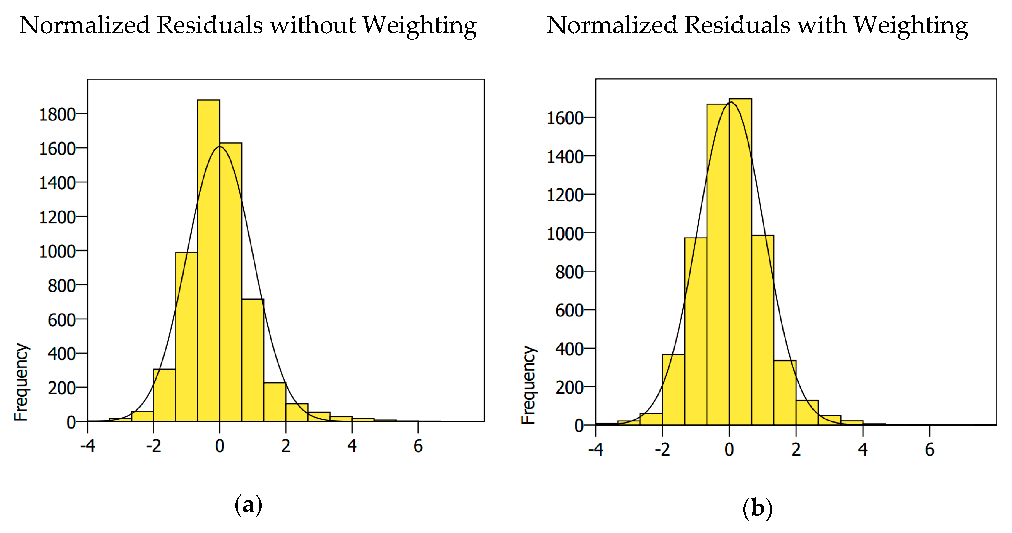
Although useable results were achieved with and without it, the Site 2 experiment illustrated the potentially significant impact on mensuration that can be made by including the uncertainty of each point as input in the algorithm. The RMSE was lower for each component, X, Y, and Z, when incorporating weights into the mensuration algorithm. Similarly, mean error magnitudes and standard deviations were generally lower when weighting. While rigorous point coordinate uncertainty requires navigation uncertainty metadata, which may preclude use by some practitioners, surrogate generic methods based on manufacturer-specified scanner encoder uncertainty, range uncertainty, and estimates of platform exterior orientation uncertainty may be as effective as rigorous physical modeling. Users are encouraged to explore either option for their systems, since beyond the benefits of carrying forward propagated uncertainties for post-processing and analysis, they also increase the accuracy of general location measurement, and avoid the reduced point cloud density and target-placement restriction associated with more naïve methods, such as point removal based on, e.g., long range or across-track distance.

The targets had some, albeit minor, drawbacks. For sparse point clouds, the targets generated noticeable systematic error in the form of lower Z coordinates relative to denser point clouds (and check point coordinates). This may be remedied by constraining tilt to zero, the approach used in the presented Site 1 experiment, since the ground was flat and level at the study site. However, on sloped ground one may need to level the targets when placing them or record the tilt to enable constraint to non-zero values.

Black tape was placed on the targets for use in fusion with photogrammetry. While it was effective in its purpose, drop-outs (no point returned) were observed for some points falling on the tape (some of these voids are visible in Figure 4a). Although this did not seem to have a significant effect on the mensuration of the targets in the point clouds, it could be remedied by using a different colored tape or only placing tape on targets that must be seen from imagery. Another approach the present authors utilized is the placement of flat targets on the ground next to the target (e.g., adjacent to the north facet) to obtain more reliable height, the weakest-resolved component for the targets. The targets were very light weight, since they were made from corrugated plastic. In windy conditions, they must be staked to the ground, or, depending on the ground composition, secured with sandbags on the corners.

The design of our targets precluded viewing any monument, such as capped rebar, underneath the targets when placed. To place a target associated with a monumented point, an effective approach has been to place a tripod with a leveled and centered optical-plummet tribrach over the monumented point, then place the target above it, centering the reference point of the pyramid visually using the tribrach. Height was measured using tape and checked using the design specifications of the target (0.4 m). The target points were easily and rapidly manually extracted from point clouds, and non-target and dubious points were identified and culled using tests based on Equations (6) and (7). However, for a large number of targets, manual extraction can be somewhat time consuming. Future work will include the development of automatic identification and extraction of target points to include a RANSAC-approach to discriminate target points and identify outliers.

5. Conclusions

Laser scanning from unoccupied aerial systems (UAS) is gaining popularity due to improved safety and lower entry costs relative to conventional large piloted systems. Compared to Structure from Motion (SfM) photogrammetry from UAS, UAS lidar offers improved processing speed and robustness of generating 3D models, and penetration of vegetation gaps for capturing terrain and production of, e.g., canopy height models. Like all geospatial data, point clouds and 3D models often require artificial targets identifiable within the products to enable accuracy assessment, calibration, adjustment, and fusion. In SfM photogrammetry, easily-manufactured flat targets with photo-identifiable markings are adequate for precisely measuring coordinates within the imagery towards 3D measurement of locations within the derived production. In UAS lidar, analogous flat intensity-based targets are often not effective, since intensity values may not allow for accurate discrimination of target points within the scene, and the distribution of target points may bias horizontal component measurements. This study introduced a new structure-based target method and associated rigorous mensuration algorithm to address this issue. The experiments presented here, with collection carried out at different sites under different flight configurations, illustrate that the developed targets are a viable method for mensuration in UAS-lidar point clouds.

The targets in this study were developed based on necessity, since the vast majority of research carried out with the UAS laser scanner involves surveys over rural, often highly vegetated areas. There are typically no artificial structures to enable mensuration, and intensity-based targeting is not effective due to the characteristics of the lidar system intensity measurements, and the reflectivity of the scenes (e.g., Figure 5). The goal in development was to create portable, multimodal (i.e., useful for photography and lidar) markers to allow reliable full 3D mensuration within UAS lidar point clouds. Beyond the presented experiments, the targets have been used in various environments, including agricultural, coastal, wetland, and diverse forested areas around Florida, and with different scanners, including the Velodyne VLP-16 LW, HDL-32E, and VLP-32C. Under typical VLP-16 scanning mission parameters (40 m or less AGL, 5-10 m/s speed, 50% nominal overlapping swaths), the targets are readily identifiable and their 3D location measurable. The only environment precluding their use has been under dense canopy, where too few points are found on the target for reliable application of the mensuration algorithm. They have been used effectively for accuracy assessment (as reported here), in situ boresight calibration, and for aligning swaths via naïve strip adjustment.

References

1. Pilarska, M.; Ostrowski, W.; Bakuła, K.; Górski, K.; Kurczyński, Z. The potential of light laser scanners developed for unmanned aerial vehicles—The review and accuracy. Int. Arch. Photogramm. Remote Sens. Spat. Inf. Sci. 2016, 62, 87–95. [Google Scholar] [CrossRef] [Green Version]
2. Starek, M.; Jung, J. The state of lidar for UAS applications. Lidar’s next geospatial frontier. UAS Spec. GIM Int. 2015, 29, 25–27. [Google Scholar]
3. Lin, Y.; Hyyppä, J.; Jaakkola, A. Mini-UAV-borne LiDAR for fine-scale mapping. IEEE Geosci. Remote Sens. Lett. 2011, 8, 426–430. [Google Scholar] [CrossRef]
4. Wallace, L.; Lucieer, A.; Watson, C.; Turner, D. Development of a UAV-LiDAR system with application to forest inventory. Remote Sens. 2012, 4, 1519–1543. [Google Scholar] [CrossRef] [Green Version]
5. Rodarmel, C.; Lee, M.; Gilbert, J.; Wilkinson, B.; Theiss, H.; Dolloff, J.; O’Neill, C. The Universal Lidar Error Model. Photogramm. Eng. Remote Sens. 2015, 81, 543–556. [Google Scholar] [CrossRef]
6. Jozkowa, G.; Toth, C.; Grejner-Brzezinskaa, D. UAS Topographic Mapping with Velodyne LiDAR Sensor. ISPRS Ann. Photogramm. Remote Sens. Spat. Inf. Sci. 2016, 3, 201–208. [Google Scholar] [CrossRef]
7. American Society for Photogrammetry and Remote Sensing (ASPRS), Summary of Research and Development Efforts Necessary for Assuring Geometric Quality of Lidar Data. Available online: https://www.asprs.org/wp-content/uploads/LidarResearchGuidelines_v1.0.pdf (accessed on 12 September 2019).
8. Habib, A.; Kersting, A.; Shaker, A.; Yan, W. Geometric Calibration and Radiometric Correction of LiDAR Data and Their Impact on the Quality of Derived Products. Sensors 2011, 11, 9069–9097. [Google Scholar] [CrossRef] [PubMed] [Green Version]
9. Habib, A.; Kersting, A.; Ruifang, Z.; Al-Durgham, M.; Kim, C.; Lee, D. LiDAR Strip Adjustment Using Conjugate Linear Features in Overlapping Strips. In Proceedings of the International Archives of Photogrammetry, Remote Sensing and Spatial Information Sciences, Beijing, China, 3–11 July 2008. [Google Scholar]
10. Rusinkiewicz, S.; Levoy, M. Efficient Variants of the ICP Algorithm. In Proceedings of the 3rd International Conference on 3D Digital Imaging and Modeling, Quebec City, QC, Canada, 28 May–1 June 2001; pp. 145–152. [Google Scholar]
11. Csanyi, N.; Toth, C. Improvement of Lidar Data Accuracy Using Lidar-Specific Ground Targets. Photogramm. Eng. Remote Sens. 2007, 73, 385–396. [Google Scholar] [CrossRef] [Green Version]
12. Bethel, J.; van Gelder, B.; Cetin, A. Corridor Mapping Using Aerial Technique. In FWHA/INDOT/JTRP-2006/23: Final Report to Indiana Department of Transportation; Indiana Department of Transportation: West Lafayette, Indiana, 2006; 94p. [Google Scholar]
13. Gruen, A. Adaptive Least Squares Correlation: A Powerful Image Matching Technique. South Afr. J. Photogramm. Remote Sens. Cartogr. 1985, 14, 175–187. [Google Scholar]
14. Canavosio-Zuzelski, R.; Hogarty, J.; Rodarmel, C.; Lee, M.; Braun, A. Assessing Lidar Accuracy with Hexagonal Retro-reflective Targets. Photogramm. Eng. Remote Sens. 2013, 79, 663–670. [Google Scholar] [CrossRef]
15. Sampath, A.; Heidemann, K.; Stensaas, G.; Christopherson, J. ASPRS Research on Quantifying the Geometric Quality of Lidar Data. Photogramm. Eng. Remote Sens. 2014, 80, 201–205. [Google Scholar]
16. Bakula, K.; Salach, A.; Wziatek, D.; Ostrowski, W.; Gorski, K.; Kurczynski, Z. Evaluation of the Accuracy of Lidar Data Acquired using a UAS for Levee Monitoring: Preliminary Results. Int. J. Remote Sens. 2017, 38, 2921–2937. [Google Scholar] [CrossRef]
17. Wallace, L.; Lucieer, A.; Watson, C.; Malenovsky, Z.; Turner, D.; Vopenka, P. Assessment of Forest Structure Using Two UAV Techniques: A Comparison of Airborne Laser Scanning and Structure from Motion (SfM) Point Clouds. Forests 2016, 7, 62. [Google Scholar] [CrossRef] [Green Version]
18. Kidd, J. Performance Evaluation of the Velodyne VLP-16 System for Surface Feature Surveying. Master’s Thesis, University of New Hampshire, Durham, NH, USA, 2017. [Google Scholar]
19. Graham, L. Drone LIDAR Considerations. In Proceedings of the Florida ASPRS Lidar Workshop, Apopka, FL, USA, 16 November 2018; pp. 312–367. [Google Scholar]
20. Wolf, P.; Dewitt, B.; Wilkinson, B. Elements of Photogrammetry with Applications in GIS, 4th ed.; McGraw-Hill Education: New York, NY, USA, 2014; pp. 5785–5792. [Google Scholar]
21. Fischler, M.; Bolles, R. Random sample consensus: A paradigm for model fitting with applications to image analysis and automated cartography. Commun. ACM 1981, 24, 381–395. [Google Scholar] [CrossRef]
Figure 1. The unoccupied aerial systems (UAS) laser scanning system used in the study.
Remotesensing 11 03019 g001
Figure 2. The structural targets. (a) A field-deployed target with dimensions. (b) The 22 folded targets stacked. Note the 1 ft (30.48 cm) engineer scale for size reference.
Remotesensing 11 03019 g002
Figure 3. The initial location and angular orientation of the target template.
Remotesensing 11 03019 g003
Figure 4. The same target points shown at the same scale for the same area colored by height (a) and by intensity (b), illustrating the benefit of using the structure for target point identification. Brightness histograms were manipulated in each to best distinguish target points. The scale bar spans 0.5 m.
Remotesensing 11 03019 g004
Figure 5. Point cloud in the neighborhood of the same pyramidal target (lower portion) and flat paper plate (upper portion) shown at the same scale for the same area (mowed grass) colored by co-aligned imagery (a) and by intensity (b), illustrating the difficulty discriminating points by intensity. Brightness histograms were manipulated in each to best distinguish target points. The scale bar spans 2 m.
Remotesensing 11 03019 g005
Figure 6. Site 1, located in Jonesville, Florida. Primary collection flight paths are indicated by black dashed lines. Gray dashed lines indicate turns where data were also collected. Targets appear as white triangles.
Remotesensing 11 03019 g006
Figure 7. Site 2, located in Ordway Swisher Biological Station, Melrose, Florida. Primary collection flight paths are indicated by black dashed lines. Light gray dashed lines indicate turns where data were also collected. The white triangle symbols are approximate target locations.
Remotesensing 11 03019 g007
Figure 8. Example of point distributions on a target for the tested point spacings at Site 1 colored by height (z). The wireframe template is positioned based on the 2 cm spacing solution.
Remotesensing 11 03019 g008
Figure 9. Position root mean square error (RMSE) based on ground-surveyed target coordinates at Site 1 for various point spacing configurations.
Remotesensing 11 03019 g009
Figure 10. Comparison of horizontal errors without (a) and with weighting (b) incorporated into the mensuration algorithm.
Remotesensing 11 03019 g010
Figure 11. Comparison of vertical errors without (a) and with weighting (b) incorporated into the mensuration algorithm.
Remotesensing 11 03019 g011
Figure 12. Histograms of normalized residuals for the unweighted (a) and weighted (b) solutions with normal distribution overlays. The abscissas show standard deviations from zero.
Remotesensing 11 03019 g012