NO2 Retrieval from the Environmental Trace Gases Monitoring Instrument (EMI): Preliminary Results and Intercomparison with OMI and TROPOMI


 ,
,
Abstract

1. Introduction
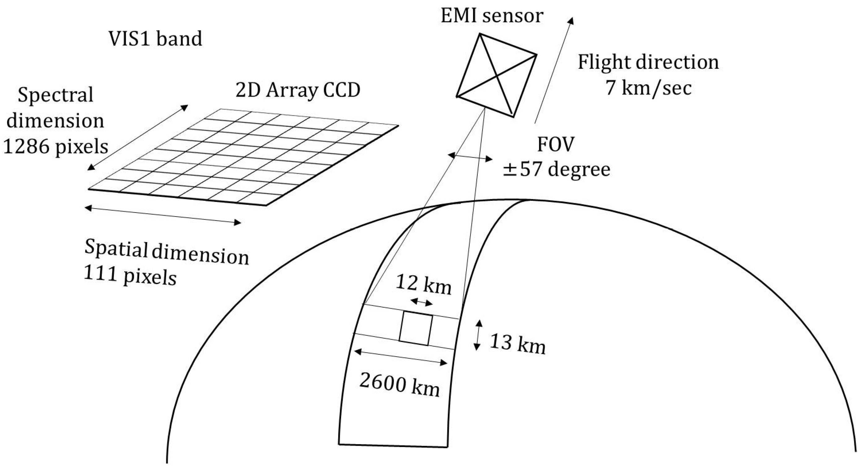
2. Data
3. EMI NO2 Retrieval Algorithm
3.1. Spectral Fitting
3.1.1. Wavelength Calibration
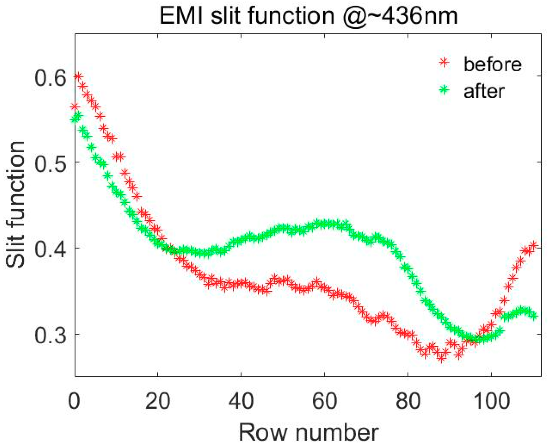
3.1.2. Slit Function Treatment
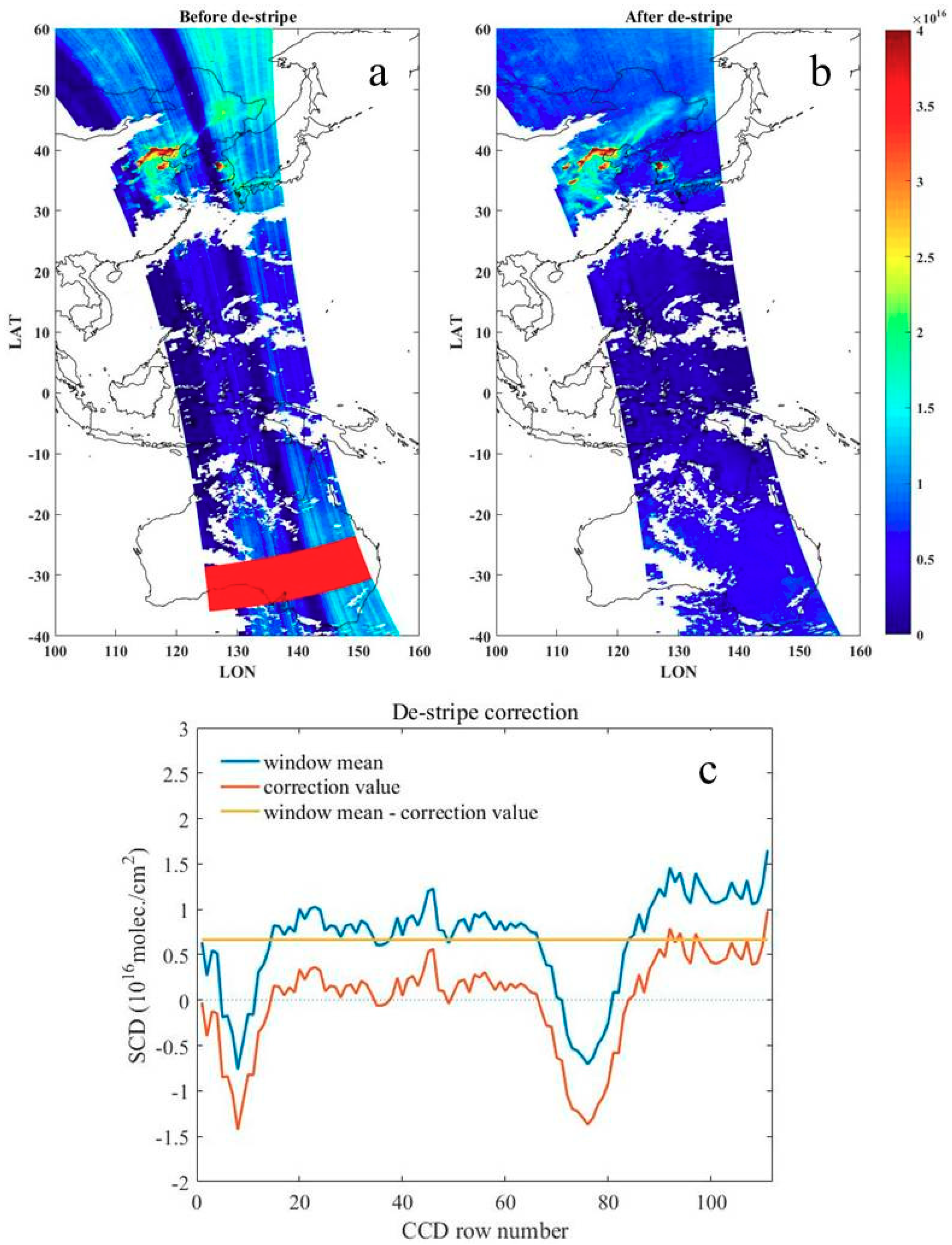
3.1.3. De-Stripe Correction
3.2. Stratosphere-Troposphere Separation (STS)
3.3. AMF Calculation
4. Results
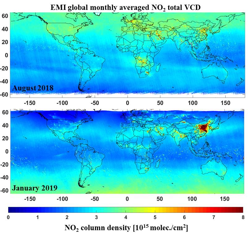
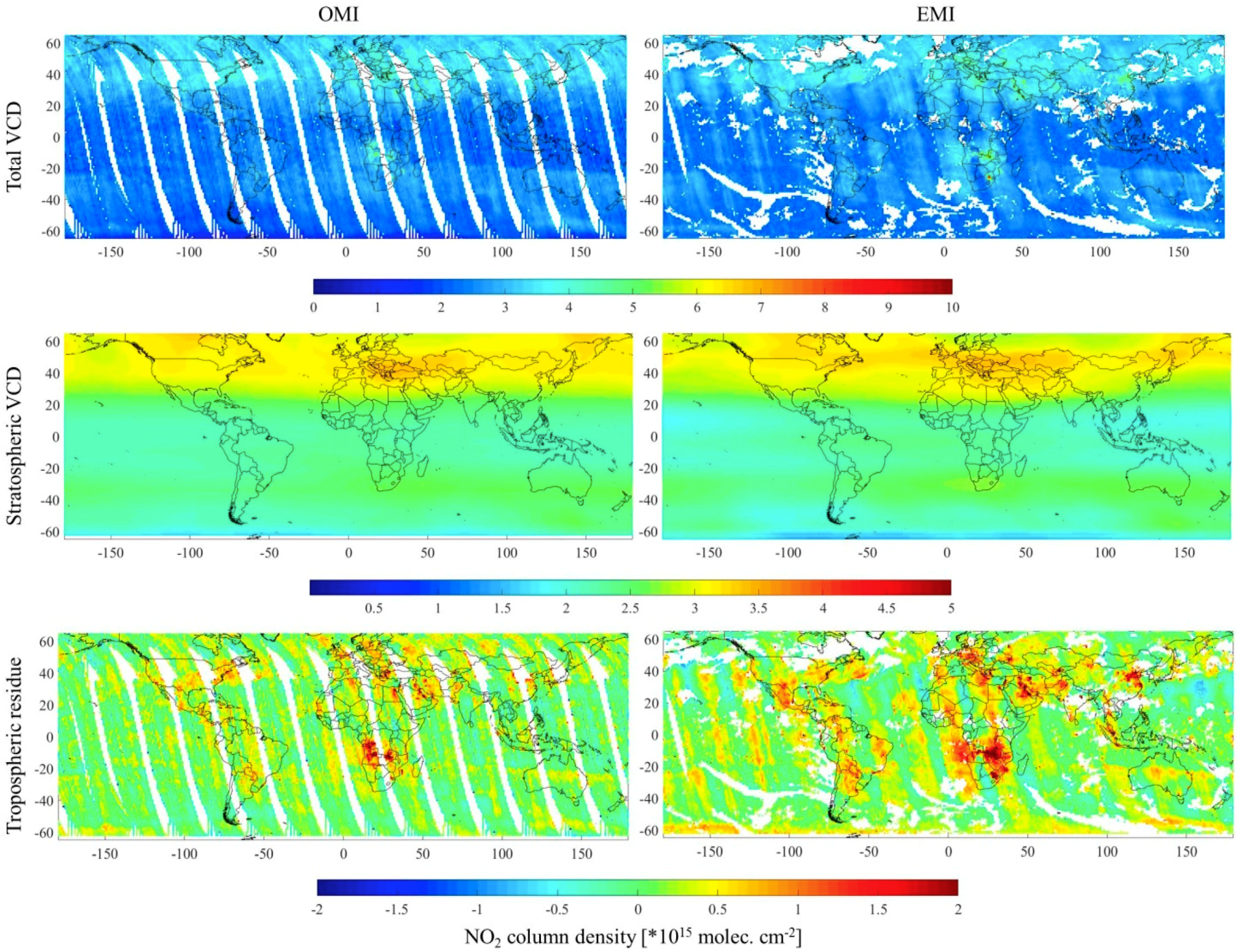
4.1. Total VCD
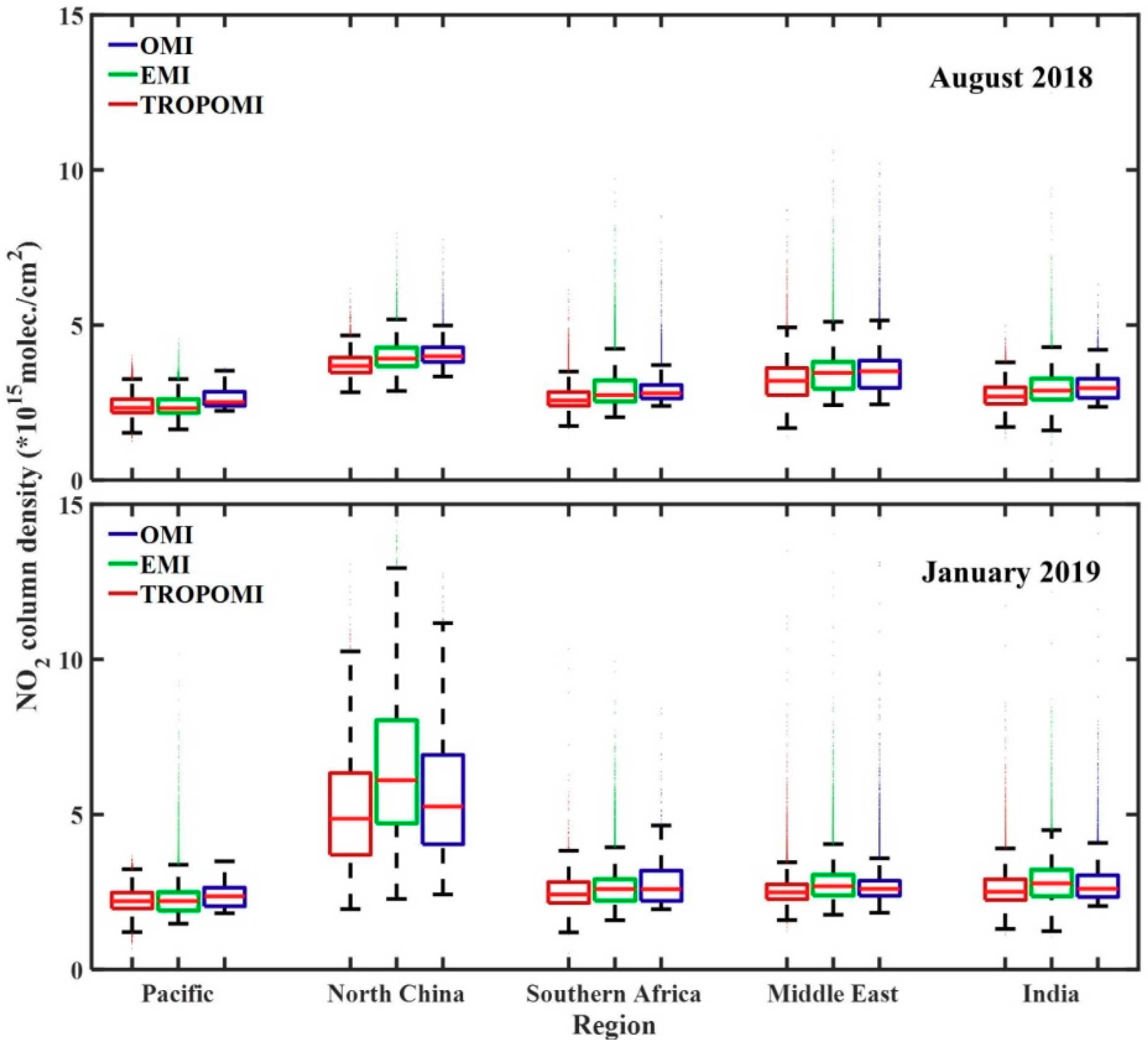
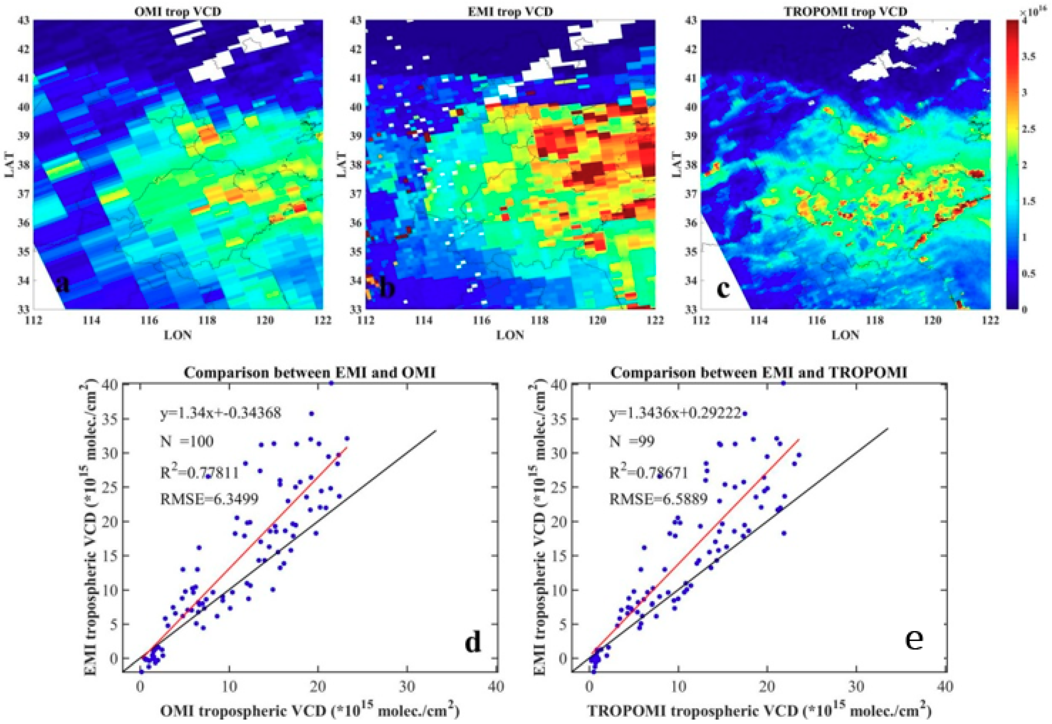
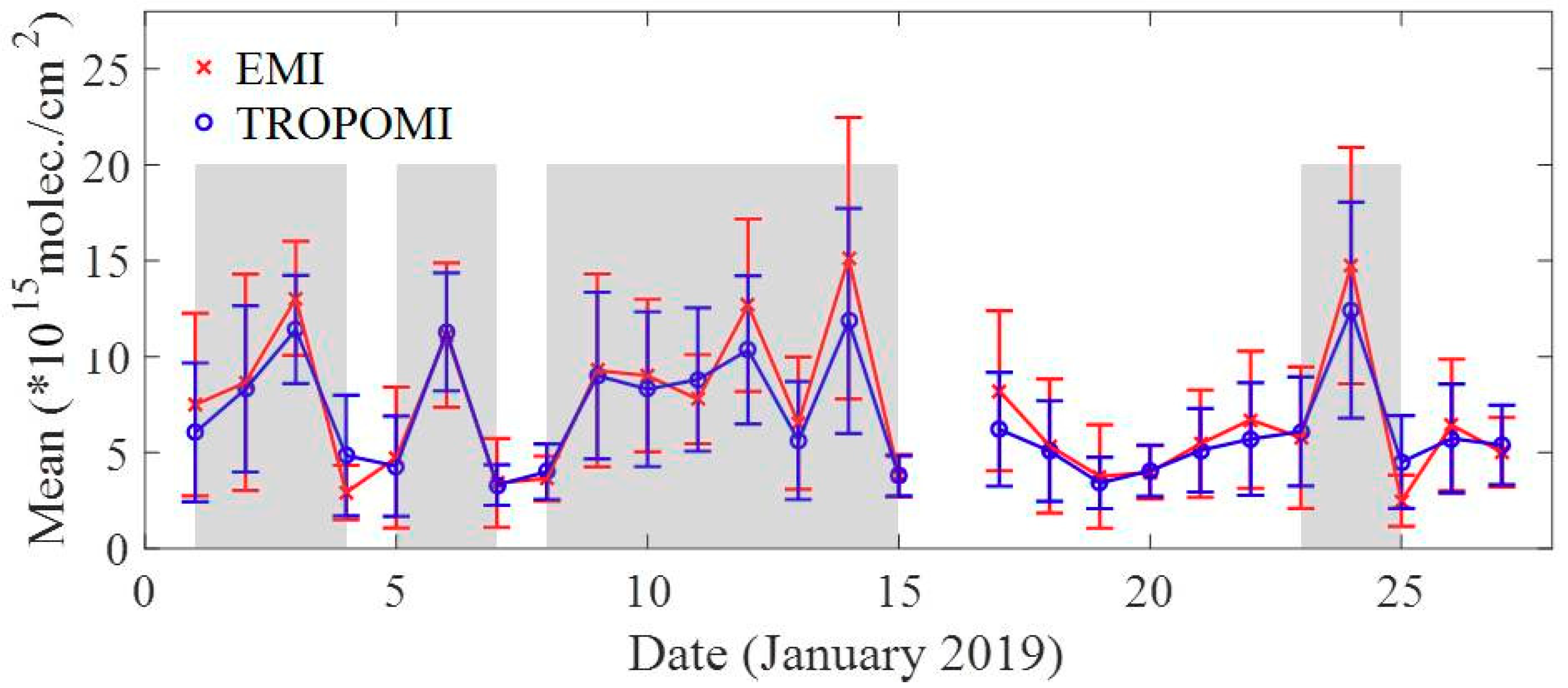
4.2. Tropospheric VCD
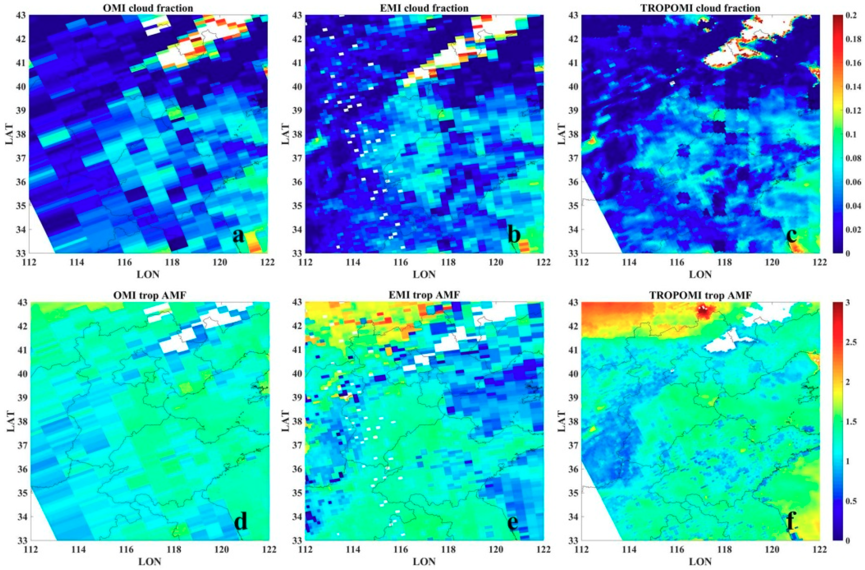
4.3. Application Case
5. Summary and Conclusions
Author Contributions
Funding
Acknowledgments
Conflicts of Interest
References
- Solomon, S. Stratospheric ozone depletion: A review of concepts and history. Rev. Geophys. 1999, 37, 275–316. [Google Scholar] [CrossRef]
- Duncan, B.N.; Yoshida, Y.; Olson, J.R.; Sillman, S.; Martin, R.V.; Lamsal, L.; Hu, Y.; Pickering, K.E.; Retscher, C.; Allen, D.J. Application of omi observations to a space-based indicator of no x and VOC controls on surface ozone formation. Atmos. Environ. 2010, 44, 2213–2223. [Google Scholar] [CrossRef]
- Lei, H.; Wang, J.X.L. Sensitivities of nox transformation and the effects on surface ozone and nitrate. Atmos. Chem. Phys. 2014, 14, 1385–1396. [Google Scholar] [CrossRef]
- Seinfeld, J.H.; Pandis, S.N. Atmospheric Chemistry and Physics: From Air Pollution to Climate Change; Wiley: Hoboken, NJ, USA, 2016. [Google Scholar]
- Li, L.J.; Tang, P.; Cocker, D.R. Instantaneous nitric oxide effect on secondary organic aerosol formation from m-xylene photooxidation. Atmos. Environ. 2015, 119, 144–155. [Google Scholar] [CrossRef]
- Van Geffen, J.H.G.M.; Boersma, K.F.; Van Roozendael, M.; Hendrick, F.; Mahieu, E.; De Smedt, I.; Sneep, M.; Veefkind, J.P. Improved spectral fitting of nitrogen dioxide from omi in the 405–465 nm window. Atmos. Meas. Tech. 2015, 8, 1685–1699. [Google Scholar] [CrossRef]
- Richter, A.; Burrows, J.P.; Nuss, H.; Granier, C.; Niemeier, U. Increase in tropospheric nitrogen dioxide over China observed from space. Nature 2005, 437, 129–132. [Google Scholar] [CrossRef]
- Zhang, L.; Lee, C.S.; Zhang, R.; Chen, L. Spatial and temporal evaluation of long term trend (2005–2014) of omi retrieved no 2 and so 2 concentrations in henan province, china. Atmos. Environ. 2017, 154, 151–166. [Google Scholar] [CrossRef]
- Souri, A.H.; Choi, Y.; Jeon, W.; Woo, J.H.; Zhang, Q.; Kurokawa, J. Remote sensing evidence of decadal changes in major tropospheric ozone precursors over east asia. J. Geophys. Res. Atmos. 2017, 122, 2474–2492. [Google Scholar] [CrossRef]
- Georgoulias, A.K.; van der A, R.J.; Stammes, P.; Boersma, K.F.; Eskes, H.J. Trends and trend reversal detection in 2 decades of tropospheric no2 satellite observations. Atmos. Chem. Phys. 2019, 19, 6269–6294. [Google Scholar] [CrossRef]
- Si, Y.D.; Li, S.S.; Chen, L.F.; Yu, C.; Wang, H.M.; Wang, Y.P. Impact of precursor gases and meteorological variables on satellite-estimated near-surface sulfate and nitrate concentrations over the north china plain. Atmos. Environ. 2019, 199, 345–356. [Google Scholar] [CrossRef]
- Burrows, J.P.; Weber, M.; Buchwitz, M.; Rozanov, V.; Ladstatter-Weissenmayer, A.; Richter, A.; DeBeek, R.; Hoogen, R.; Bramstedt, K.; Eichmann, K.U.; et al. The global ozone monitoring experiment (gome): Mission concept and first scientific results. J. Atmos. Sci. 1999, 56, 151–175. [Google Scholar] [CrossRef]
- Beirle, S.; Platt, U.; Wenig, M.; Wagner, T. Weekly cycle of no2 by gome measurements: A signature of anthropogenic sources. Atmos. Chem. Phys. 2003, 3, 2225–2232. [Google Scholar] [CrossRef]
- Bovensmann, H.; Burrows, J.P.; Buchwitz, M.; Frerick, J.; Noel, S.; Rozanov, V.V.; Chance, K.V.; Goede, A.P.H. Sciamachy: Mission objectives and measurement modes. J. Atmos. Sci. 1999, 56, 127–150. [Google Scholar] [CrossRef]
- Levelt, P.F.; Van den Oord, G.H.J.; Dobber, M.R.; Malkki, A.; Visser, H.; de Vries, J.; Stammes, P.; Lundell, J.O.V.; Saari, H. The ozone monitoring instrument. IEEE Trans. Geosci. Remote 2006, 44, 1093–1101. [Google Scholar] [CrossRef]
- Fioletov, V.E.; McLinden, C.A.; Krotkov, N.; Moran, M.D.; Yang, K. Estimation of SO2 emissions using omi retrievals. Geophys. Res. Lett. 2011, 38. [Google Scholar] [CrossRef]
- Callies, J.; Corpaccioli, E.; Eisinger, M.; Hahne, A.; Lefebvre, A. Gome-2-Metop’s second-generation sensor for operational ozone monitoring. ESA Bull. Eur. Space 2000, 102, 28–36. [Google Scholar]
- Munro, R.; Lang, R.; Klaes, D.; Poli, G.; Retscher, C.; Lindstrot, R.; Huckle, R.; Lacan, A.; Grzegorski, M.; Holdak, A.; et al. The gome-2 instrument on the metop series of satellites: Instrument design, calibration, and level 1 data processing—An overview. Atmos. Meas. Tech. 2016, 9, 1279–1301. [Google Scholar] [CrossRef]
- Veefkind, J.P.; Aben, I.; McMullan, K.; Forster, H.; de Vries, J.; Otter, G.; Claas, J.; Eskes, H.J.; de Haan, J.F.; Kleipool, Q.; et al. Tropomi on the esa sentinel-5 precursor: A gmes mission for global observations of the atmospheric composition for climate, air quality and ozone layer applications. Remote Sens. Environ. 2012, 120, 70–83. [Google Scholar] [CrossRef]
- Griffin, D.; Zhao, X.; McLinden, C.A.; Boersma, F.; Bourassa, A.; Dammers, E.; Degenstein, D.; Eskes, H.; Fehr, L.; Fioletov, V.; et al. High-resolution mapping of nitrogen dioxide with tropomi: First results and validation over the canadian oil sands. Geophys. Res. Lett. 2019, 46, 1049–1060. [Google Scholar] [CrossRef]
- Zhang, C.X.; Liu, C.; Wang, Y.; Si, F.Q.; Zhou, H.J.; Zhao, M.J.; Su, W.J.; Zhang, W.Q.; Chan, K.L.; Liu, X.; et al. Preflight evaluation of the performance of the chinese environmental trace gas monitoring instrument (EMI) by spectral analyses of nitrogen dioxide. IEEE Trans. Geosci. Remote 2018, 56, 3323–3332. [Google Scholar] [CrossRef]
- Zhao, M.J.; Si, F.Q.; Zhou, H.J.; Wang, S.M.; Jiang, Y.; Liu, W.Q. Preflight calibration of the chinese environmental trace gases monitoring instrument (EMI). Atmos Meas Tech 2018, 11, 5403–5419. [Google Scholar] [CrossRef]
- Martin, R.V.; Chance, K.; Jacob, D.J.; Kurosu, T.P.; Spurr, R.J.D.; Bucsela, E.; Gleason, J.F.; Palmer, P.I.; Bey, I.; Fiore, A.M.; et al. An improved retrieval of tropospheric nitrogen dioxide from gome. J. Geophys. Res. Atmos. 2002, 107. [Google Scholar] [CrossRef]
- Boersma, K.F.; Eskes, H.J.; Veefkind, J.P.; Brinksma, E.J.; van der A, R.J.; Sneep, M.; van den Oord, G.H.J.; Levelt, P.F.; Stammes, P.; Gleason, J.F.; et al. Near-real time retrieval of tropospheric no2 from omi. Atmos. Chem. Phys. 2007, 7, 2103–2118. [Google Scholar] [CrossRef]
- Beirle, S.; Kuehl, S.; Pukite, J.; Wagner, T. Retrieval of tropospheric column densities of NO2 from combined sciamachy nadir/limb measurements. Atmos. Meas. Tech. 2010, 3, 283–299. [Google Scholar] [CrossRef]
- Boersma, K.F.; Eskes, H.J.; Dirksen, R.J.; van der A, R.J.; Veefkind, J.P.; Stammes, P.; Huijnen, V.; Kleipool, Q.L.; Sneep, M.; Claas, J.; et al. An improved tropospheric no2 column retrieval algorithm for the ozone monitoring instrument. Atmos. Meas. Tech. 2011, 4, 1905–1928. [Google Scholar] [CrossRef]
- Valks, P.; Pinardi, G.; Richter, A.; Lambert, J.C.; Hao, N.; Loyola, D.; Van Roozendael, M.; Emmadi, S. Operational total and tropospheric no2 column retrieval for gome-2. Atmos. Meas. Tech. 2011, 4, 1491–1514. [Google Scholar] [CrossRef]
- Boersma, K.F.; Eskes, H.J.; Richter, A.; De Smedt, I.; Lorente, A.; Beirle, S.; van Geffen, J.H.G.M.; Zara, M.; Peters, E.; Van Roozendael, M.; et al. Improving algorithms and uncertainty estimates for satellite no2 retrievals: Results from the quality assurance for the essential climate variables (QA4ECV) project. Atmos. Meas. Tech. 2018, 11, 6651–6678. [Google Scholar] [CrossRef]
- Liu, S.; Valks, P.; Pinardi, G.; De Smedt, I.; Yu, H.; Beirle, S.; Richter, A. An improved total and tropospheric no2 column retrieval for gome-2. Atmos. Meas. Tech. 2019, 12, 1029–1057. [Google Scholar] [CrossRef]
- Dirksen, R.J.; Boersma, K.F.; Eskes, H.J.; Ionov, D.V.; Bucsela, E.J.; Levelt, P.F.; Kelder, H.M. Evaluation of stratospheric no2 retrieved from the ozone monitoring instrument: Intercomparison, diurnal cycle, and trending. J. Geophys. Res. Atmos. 2011, 116. [Google Scholar] [CrossRef]
- Bucsela, E.J.; Krotkov, N.A.; Celarier, E.A.; Lamsal, L.N.; Swartz, W.H.; Bhartia, P.K.; Boersma, K.F.; Veefkind, J.P.; Gleason, J.F.; Pickering, K.E. A new stratospheric and tropospheric NO2 retrieval algorithm for nadir-viewing satellite instruments: Applications to omi. Atmos. Meas. Tech. 2013, 6, 2607–2626. [Google Scholar] [CrossRef]
- Beirle, S.; Hoermann, C.; Joeckel, P.; Liu, S.; de Vries, M.P.; Pozzer, A.; Sihler, H.; Valks, P.; Wagner, T. The stratospheric estimation algorithm from mainz (stream): Estimating stratospheric no2 from nadir-viewing satellites by weighted convolution. Atmos. Meas. Tech. 2016, 9, 2753–2779. [Google Scholar] [CrossRef]
- Boersma, K.F.; Eskes, H.J.; Brinksma, E.J. Error analysis for tropospheric no2 retrieval from space. J. Geophys. Res. Atmos. 2004, 109. [Google Scholar] [CrossRef]
- Lin, J.T.; Martin, R.V.; Boersma, K.F.; Sneep, M.; Stammes, P.; Spurr, R.; Wang, P.; Van Roozendael, M.; Clemer, K.; Irie, H. Retrieving tropospheric nitrogen dioxide from the ozone monitoring instrument: Effects of aerosols, surface reflectance anisotropy, and vertical profile of nitrogen dioxide. Atmos. Chem. Phys. 2014, 14, 1441–1461. [Google Scholar] [CrossRef]
- Lin, J.T.; Liu, M.Y.; Xin, J.Y.; Boersma, K.F.; Spurr, R.; Martin, R.; Zhang, Q. Influence of aerosols and surface reflectance on satellite no2 retrieval: Seasonal and spatial characteristics and implications for NOx emission constraints. Atmos. Chem. Phys. 2015, 15, 11217–11241. [Google Scholar] [CrossRef]
- Lorente, A.; Boersma, K.F.; Yu, H.; Dorner, S.; Hilboll, A.; Richter, A.; Liu, M.Y.; Lamsal, L.N.; Barkley, M.; De Smedt, I.; et al. Structural uncertainty in air mass factor calculation for NO2 and hcho satellite retrievals. Atmos. Meas. Tech. 2017, 10, 759–782. [Google Scholar] [CrossRef]
- Tong, X.D.; Zhao, W.B.; Xing, J.; Fu, W. Status and development of china high-resolution earth observation system and application. In Proceedings of the 2016 IEEE International Geoscience and Remote Sensing Symposium, Beijing, China, 10–15 July 2016; pp. 3738–3741. [Google Scholar]
- Platt, U.; Stutz, J. Differential Optical Absorption Spectroscopy: Principles and Applications; Springer: Berlin/Heidelberg, Germany, 2008. [Google Scholar]
- Vandaele, A.C.; Hermans, C.; Simon, P.C.; Carleer, M.; Colin, R.; Fally, S.; Merienne, M.-F.; Jenouvrier, A.; Coquart, B. Measurements of the NO2 absorption cross-section from 42,000 cm–1 to 10,000 cm–1 (238–1000 nm) at 220 K and 294 K. J. Quant. Spectrosc. Radiat. Transf. 1998, 59, 171–184. [Google Scholar] [CrossRef]
- Malicet, J.; Daumont, D.; Charbonnier, J.; Parisse, C.; Chakir, A.; Brion, J. Ozone uv spectroscopy. Ii. Absorption cross-sections and temperature dependence. J. Atmos. Chem. 1995, 21, 263–273. [Google Scholar] [CrossRef]
- Gordon, I.E.; Rothman, L.S.; Hill, C.; Kochanov, R.V.; Tan, Y.; Bernath, P.F.; Birk, M.; Boudon, V.; Campargue, A.; Chance, K.V.; et al. The hitran2016 molecular spectroscopic database. J. Quant. Spectrosc. Radiat. Transf. 2017, 203, 3–69. [Google Scholar] [CrossRef]
- Rothman, L.S.; Gordon, I.E.; Babikov, Y.; Barbe, A.; Benner, D.C.; Bernath, P.F.; Birk, M.; Bizzocchi, L.; Boudon, V.; Brown, L.R.; et al. The HITRAN2012 molecular spectroscopic database. J. Quant. Spectrosc. Radiat. Transf. 2013, 130, 4–50. [Google Scholar] [CrossRef]
- Pope, R.M.; Fry, E.S. Absorption spectrum (380–700 nm) of pure water. II. Integrating cavity measurements. Appl. Optics 1997, 36, 8710–8723. [Google Scholar] [CrossRef]
- Thalman, R.; Volkamer, R. Temperature dependent absorption cross-sections of O 2–O 2 collision pairs between 340 and 630 nm and at atmospherically relevant pressure. Phys. Chem. Chem. Phys. 2013, 15, 15371–15381. [Google Scholar] [CrossRef] [PubMed]
- Danckaert, T.; Fayt, C.; Van Roozendael, M.; De Smedt, I.; Letocart, V.; Merlaud, A.; Pinardi, G. QDOAS Software User Manual Version 3.2; Royal Belgian Institute for Space Aeronomy: Brussels, Belgium, 2019. [Google Scholar]
- Marchenko, S.; Krotkov, N.A.; Lamsal, L.N.; Celarier, E.A.; Swartz, W.H.; Bucsela, E.J. Revising the slant column density retrieval of nitrogen dioxide observed by the ozone monitoring instrument. J. Geophys. Res. Atmos. 2015, 120, 5670–5692. [Google Scholar] [CrossRef] [PubMed]
- van Geffen, J.H.G.M.; Eskes, H.J.; Boersma, K.F.; Maasakkers, J.D.; Veefkind, J.P. TROPOMI ATBD of the Total and Tropospheric NO2 Data Products (Issue 1.2.0); s5P-KNMI-L2-0005-RP; Royal Netherlands Meteorological Institute (KNMI): De Bilt, The Netherlands, 2018. [Google Scholar]
- Chance, K.; Kurucz, R. An improved high-resolution solar reference spectrum for earth’s atmosphere measurements in the ultraviolet, visible, and near infrared. J. Quant. Spectrosc. Radiat. Transf. 2010, 111, 1289–1295. [Google Scholar] [CrossRef]
- Beirle, S.; Lampel, J.; Lerot, C.; Sihler, H.; Wagner, T. Parameterizing the instrumental spectral response function and its changes by a super-gaussian and its derivatives. Atmos. Meas. Tech. 2017, 10, 581–598. [Google Scholar] [CrossRef]
- Spurr, R.; Christi, M. On the generation of atmospheric property jacobians from the (v)lidort linearized radiative transfer models. J. Quant. Spectrosc. Radiat. Transf. 2014, 142, 109–115. [Google Scholar] [CrossRef]
- Wang, J.; Xu, X.G.; Ding, S.G.; Zeng, J.; Spurr, R.; Liu, X.; Chance, K.; Mishchenko, M. A numerical testbed for remote sensing of aerosols, and its demonstration for evaluating retrieval synergy from a geostationary satellite constellation of geo-cape and goes-r. J. Quant. Spectrosc. Radiat. Transf. 2014, 146, 510–528. [Google Scholar] [CrossRef]
- Joiner, J.; Vasilkov, A.P. First results from the omi rotational raman scattering cloud pressure algorithm. IEEE Trans. Geosci. Remote 2006, 44, 1272–1282. [Google Scholar] [CrossRef]
- Acarreta, J.R.; De Haan, J.F.; Stammes, P. Cloud pressure retrieval using the O-2-O-2 absorption band at 477 nm. J. Geophys. Res. Atmos. 2004, 109. [Google Scholar] [CrossRef]
- Williams, J.E.; Boersma, K.F.; Le Sager, P.; Verstraeten, W.W. The high-resolution version of tm5-mp for optimized satellite retrievals: Description and validation. Geosci. Model Dev. 2017, 10, 721–750. [Google Scholar] [CrossRef]
- Kleipool, Q.L.; Dobber, M.R.; de Haan, J.F.; Levelt, P.F. Earth surface reflectance climatology from 3 years of omi data. J. Geophys Res. Atmos. 2008, 113. [Google Scholar] [CrossRef]


| Parameters | EMI | OMI-NASA [46] | TROPOMI [47] | |
|---|---|---|---|---|
| Fitting window | 405–465 nm | 402–465 nm | 405–465 nm | |
| Reference spectrum I0 | Irradiance measured on 12 June, 2018 | Monthly mean solar irradiance | Annual mean (2005) solar reference | |
| Polynomial | 5th-order | Two in seven microwindows: (402–410), (409–418), (415–425), (424–434), (433–444), (438–453), and (451–465) | 5th-order | |
| Included cross sections | CHOCHO | × | √ (296 K) | × |
| O3 | √ (223 K) | × | √ (243 K) | |
| NO2 | √ (220 K) | √ (220 K) | √ (220K) | |
| O4 | √ (293 K) | × | √ (293 K) | |
| H2O vapor | √ (280 K) | √ (280 K) | √ (280 K) | |
| H2O (liquid) | √ | × | √ (295 K) | |
| Ring Effect | √ | √Air+water | √ | |
| Offset correction | √ | × | × | |
| Parameter | Number of Nodes | Grid Values |
|---|---|---|
| SZA (°) | 16 | 0, 10, 20, 30, 40, 45, 50, 55, 60, 65, 70, 72, 74, 76, 78, 80 |
| VZA (°) | 9 | 0, 10, 20, 30, 40, 50, 60, 65, 70 |
| RAA (°) | 5 | 0, 45, 90, 135, 175 |
| Albedo | 14 | 0, 0.01, 0.025, 0.05, 0.75, 0.1, 0.15, 0.2, 0.25, 0.3, 0.4, 0.6, 0.8, 1.0 |
| Surface/Cloud pressure (hPa) | 17 | 1063.10, 1037.90, 1013.30, 989.28, 965.83, 920.58, 876.98, 834.99, 795.01, 701.21, 616.60, 540.48, 411.05, 308.00, 226.99, 165.79, 121.11 |
© 2019 by the authors. Licensee MDPI, Basel, Switzerland. This article is an open access article distributed under the terms and conditions of the Creative Commons Attribution (CC BY) license (http://creativecommons.org/licenses/by/4.0/).
Share and Cite
Cheng, L.; Tao, J.; Valks, P.; Yu, C.; Liu, S.; Wang, Y.; Xiong, X.; Wang, Z.; Chen, L. NO2 Retrieval from the Environmental Trace Gases Monitoring Instrument (EMI): Preliminary Results and Intercomparison with OMI and TROPOMI. Remote Sens. 2019, 11, 3017. https://doi.org/10.3390/rs11243017
Cheng L, Tao J, Valks P, Yu C, Liu S, Wang Y, Xiong X, Wang Z, Chen L. NO2 Retrieval from the Environmental Trace Gases Monitoring Instrument (EMI): Preliminary Results and Intercomparison with OMI and TROPOMI. Remote Sensing. 2019; 11(24):3017. https://doi.org/10.3390/rs11243017
Chicago/Turabian StyleCheng, Liangxiao, Jinhua Tao, Pieter Valks, Chao Yu, Song Liu, Yapeng Wang, Xiaozhen Xiong, Zifeng Wang, and Liangfu Chen. 2019. "NO2 Retrieval from the Environmental Trace Gases Monitoring Instrument (EMI): Preliminary Results and Intercomparison with OMI and TROPOMI" Remote Sensing 11, no. 24: 3017. https://doi.org/10.3390/rs11243017
APA StyleCheng, L., Tao, J., Valks, P., Yu, C., Liu, S., Wang, Y., Xiong, X., Wang, Z., & Chen, L. (2019). NO2 Retrieval from the Environmental Trace Gases Monitoring Instrument (EMI): Preliminary Results and Intercomparison with OMI and TROPOMI. Remote Sensing, 11(24), 3017. https://doi.org/10.3390/rs11243017