Evaluation of Six Directional Canopy Emissivity Models in the Thermal Infrared Using Emissivity Measurements

Abstract

Land surface temperature (LST) is a fundamental physical quantity in a range of different studies, for example in climatological analyses and surface–atmosphere heat flux assessments, especially in heterogeneous and complex surfaces such as vegetated canopies. To obtain accurate LST values, it is important to measure accurately the land surface emissivity (LSE) in the thermal infrared spectrum. In the past decades, different directional emissivity canopy models have been proposed. This paper evaluates six radiative transfer models (FR97, Mod3, Rmod3, 4SAIL, REN15, and CE-P models) through a comparison with in situ emissivity measurements performed using the temperature-emissivity separation (TES) method. The evaluation is done using a single set of rose plants over two different soils with very different spectral behavior. First, using an organic soil, the measurements were done for seven different observation angles, from 0° to 60° in steps of 10°, and for six different values of leaf area index (LAI). Taking into account all LAIs, the bias (and root mean square error, RMSE) obtained were 0.003 (±0.006), −0.004 (±0.005), −0.009 (±0.011), 0.005 (±0.007), 0.004 (±0.007), and 0.005 (±0.007) for FR97, Mod3, Rmod3, 4SAIL, REN 15, and CE-P models, respectively. Second, using an inorganic soil, the measurements were done for six different LAIs but for two different observation angles: 0° and 55°. The bias (and RMSE) obtained were 0.012 (±0.014), 0.004 (±0.007), −0.020 (±0.035), 0.016 (±0.017), 0.013 (±0.015), 0.013 (±0.015) and for FR97, Mod3, Rmod3, 4SAIL, REN15, and CE-P models, respectively. Overall, the Mod3 model appears as the best model in comparison to the TES emissivity reference measurements.

1. Introduction

Land surface temperature (LST) is a fundamental physical quantity in a range of diverse studies on physical phenomena, such as climatological analyses, surface-atmosphere heat energy interactions (e.g., evapotranspiration), to mention some examples [1,2]. Atmospheric and surface emissivity corrections are the main factors that affect an accurate retrieval of LST for data acquired from satellite sensors in the thermal infrared spectrum (TIR). Then, a precise characterization of the land surface emissivity (LSE) is important for the LST retrieval [3]. Moreover, the emissivity spectrum is a characteristic feature of each surface, so it could be used to differentiate between different soil classes [4,5], vegetated species [6,7], and other surfaces, such as inland waters or manmade materials.

The emissivity of homogeneous surfaces such as bare soils and rocks is relatively well-known. A number of previous works have analyzed the dependence of soil emissivity on viewing angle [8,9,10] and soil moisture [11,12,13] from an empirical perspective. Different theoretical models based on the Mie theory have been proposed to predict the emissivity of these kind of surfaces considering the refraction index, the size particle distribution, etc., [14,15] that have been recently compared with laboratory data [16,17].

However, for heterogeneous surfaces the emissivity modeling is a more challenging point because of its structural complexity. This difficulty is found over canopy areas. For canopy areas, the emissivity modeling is affected by the interaction of the surface-leaving radiance and the plant elements, and between the different layers of the plant. For that, it is necessary to consider the multiple reflections that take place inside the canopy when the emissivity is being modeled. Different models that estimate the directional canopy emissivity can be found in the literature of the last decades [18]. Mainly, these models can be classified in three types: bidirectional reflectance distribution function models, BRDF [19], geometrical models, GM [20,21], and radiative transfer models, RTM [22,23,24,25]. BRDF models make use of a linear combination of defined kernels in order to obtain the directional-hemispherical reflectance, which is later used to obtain the directional emissivity by applying the Kirchhoff’s law. GMs are based on the assessment of the proportions of the different parts of the canopy actually seen at the instrument viewpoint. To apply the GMs, it is required the prior knowledge of the dimension of the canopy elements viewed by the sensor. With that, the emissivity is estimated taking into account the contribution of each one of the elements to the total measured radiance. Lastly, RTMs obtain the directional emissivity from the simulation of the radiative interaction with the different components of the canopy at the different layers. It is used the directional gap frequency, which is based on the leave density function, in order to estimate the radiance at the top of the canopy cover and, then, the emissivity. These models differ from the GMs in the fact that the canopy is not considered as an opaque medium.

In this work, the different RTMs proposed by François et al. in [22] (FR97 model), François in [23] (Mod3 model), Shi in [26] (Rmod3 model), Ren et al. in [27] (REN15 model), and Cao et al. in [28] (CE-P model) are analyzed. Also, the 4SAIL (scattering by arbitrarily inclined leaves) [25] is used in this study, since it is extensively used as a reference for other simpler algorithms. Different authors compared simulated emissivity values obtained with these models in order to analyze the emissivity spectrum for various leaf area index (LAI) values over a canopy. For example, Sobrino et al. [29] determined that for the FR97 model, the emissivity increases with the observation angle for LAI values lower or equal to 1.0 m²/m². However, for LAI values higher than 1.0 m²/m², the emissivity decreases when the observation angle increases. Ren et al. [27] compared the differences between FR97 and Mod3 models with simulated values obtained with the 4SAIL model, which is used as a reference. It is concluded that, since the Mod3 model does not take into account the multiple interactions between the different layers of vegetation, the emissivity values obtained with this method are lower than those obtained with the FR97 model, but both underestimate the values given by the 4SAIL model. Moreover, Ren et al. [27] proposed new values for the cavity effect term of the FR97 model to make their values closer with those given by 4SAIL, especially for high observation zenith angles. Finally, Cao et al. [28] compared simulated measurements of the CE-P with 4SAIL simulations, obtaining absolute differences lower than 0.002 between both models.

To our knowledge, there are no previous works that have analyzed the variation of canopy emissivity with observation angle using in situ measurements with real canopies. However, some studies have analyzed the emissivity of canopies based on in situ nadir measurements. For example, Neinavaz et al. [30] found a relationship between the emissivity and LAI of different canopies for nadir hyperspectral measurements; this relationship allowed obtaining the LAI of a plant from a combination of emissivity measurements in different spectral bands provided that LAI was not very high. Also, in Neinavaz et al. [31], at-nadir canopy emissivity spectra of different species were analyzed, resulting that in the spectral range between 8 |ìm and 10 |ìm the discrimination among species is more accurate. Moreover, it was found that emissivity values increase with increasing LAI, but from LAI values of 4 m²/m² the emissivity takes a nearly constant value for higher LAI values.

Thus, the objective of this paper is twofold. First, to use a set of in situ emissivity measurements acquired on a canopy at different viewing observation conditions and for LAI values in the range 0.5 m²/m² to 3.3 m²/m², for studying the emissivity change with viewing angle and vegetation amount. Second, to compare and evaluate the four RTM-type algorithms described above using these in situ data, in order to investigate their predictive power in the assessment of canopy emissivity. All emissivity measurements were acquired using the temperature-emissivity separation (TES) algorithm [32] adapted to multiband ground radiometers CIMEL Electronique CE312-2 [33].

2. Experimental Setup and Data Processing

The experiment took place at the Facultat de Física of the Universitat de València, Spain (13°30′25″ N, 0°25′13″ W), using a goniometer placed on the roof of the building. It was carried out in two different periods, first on the months of October and November, 2017, and second on four consecutive days, from 29 May to 1 June 2019. For both periods the measurements were made on cloudless days. The same plant species (a set of rose plants) were used in the two periods, but different soil backgrounds were selected for each case: organic soil in the first period and inorganic soil (sand) in the second one. A six-band Cimel Electronique CE312-2 radiometer [34] was used to make the measurements over the sample of the study. In the first period, seven different observation angles, varying from 0° to 60° in steps of 10°, were considered. In order to reduce the LAI values of the sample, the plant leaves were cut off when the set of measurements at different observation angles was done. The measurements were repeated for six different values of LAI ranging from 2.8 m²/m² to 0.5 m²/m², which were measured with Android app Pocket-LAI [35]. For the second period, a similar procedure was carried out. This time, we considered observation angles of nadir and 55°, with LAI measured values ranging from 3.3 m²/m² to 0.6 m²/m². During the second experiment, the number of observation angles was reduced because of two reasons: First, in García-Santos et al. [10] it was found that the decrease of emissivity on sand sample was observed for observation angles higher than 40°. Second, no significant variation with angle was observed in the emissivity measurements during the first period. Then, the measurements were repeated with just two observation angles because no significant differences with angle were expected for lower observation angles.

In order to assure enough measurements for adequate statistics, the number of radiance measurements was of 15 for each band, observation angle, and LAI value. Therefore, a total of 630 measurements of the sample for each band for the first period and 180 measurements for each band for the second period were used in this study. The height of the radiometer was adjusted for each observation angle in order to assure a constant field of view of 0.048 m². Also, a second six-band Cimel CE312-2 radiometer was used to measure the hemispherical downwelling radiance, simultaneously to each measurement, making use of a Labsphere golden panel with high reflectivity in the TIR [36]. The experimental setup is shown in Figure 1.

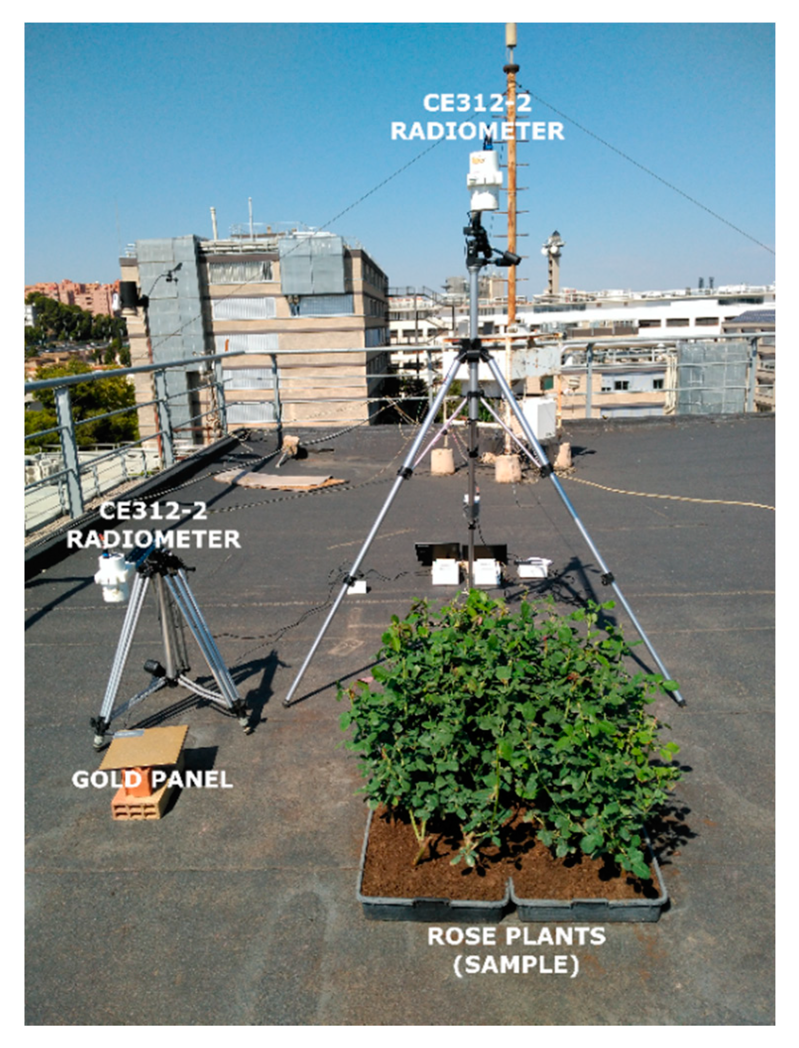
2.1. Cimel ElectroniqueCE312-2

Sample radiances and downwelling hemispheric radiances were measured using two Cimel Electronique CE312-2 radiometers. This field instrument focuses its six spectral bands in the TIR spectrum, covering from 8 to 13 µm. Its first band is a wide band covering all the wavelength range (band 1: 8–13.3 µm), whereas the other five bands are distributed along this spectral range: 10.9–11.7 µm (band 2), 10.2–11.0 µm (band 3), 9.0–9.3 µm (band 4), 8.5–8.9 µm (band 5), and 8.3–8.6 µm (band 6). These five narrow bands are coincident with the ASTER sensor TIR bands. The CE312-2 radiometer has an accuracy of 0.2 K according to the manufacturer and a field of view of 10°. Moreover, both radiometers were calibrated against the National Physical Laboratory (NPL) ammonia heat-pipe reference blackbody during the Fiducial Reference Measurements for validation of surface temperature from satellites (FRM4STS) experiment in June 2016. It was obtained a root mean square error (RMSE) between 0.06 and 0.10 K for bands 1 to 3 and a RMSE between 0.13 and 0.23 K for bands 4 to 6 [33,37].

In order to retrieve emissivity values from sample radiance measurements, it is required to measure the hemispheric downwelling radiance. For that reason, it was measured over an Infragold Reflectance Target (IRT-94-100) made by Labsphere [36]. This target is a high diffuse reflectivity gold panel, with reflectivity values close to 0.92 for the six spectral bands of the CE312-2 radiometer [38].

2.2. TES Algorithm

The TES method [31] was first devised and extensively applied to ASTER sensor [39,40,41], but because of the similarities between the ASTER and the CE312-2 spectral bands, it can also be applied to the latter using the same empirical equations for both instruments [33,42]. The TES algorithm starts with the normalized emissivity method (NEM) [43] using the at-surface and the downwelling radiance measurements taken by the five ASTER TIR channels. NEM calculates five different temperatures assuming a common initial emissivity guess value, typically 0.990. The highest temperature value is assumed as a first-guess land surface temperature, which is known as T_NEM. With the obtained T_NEM, the so-called NEM emissivity $\left({\epsilon }_{NEM,i}\right)$ is retrieved for each spectral band using the corresponding at-surface and downwelling radiances. Dividing each ${\epsilon }_{NEM,i}$ by the mean value of the NEM emissivities, the temperature-independent ${\beta }_i$ index is calculated. Next, an empirical relation relating the minimum emissivity ${\epsilon }_{min}$ with the maximum-minimum emissivity difference (MMD) is used to obtain ${\epsilon }_{min}$. For that, the MMD is obtained from the difference of the maximum and minimum value of ${\beta }_i$ index. To avoid possible systematic errors in the TES results, the empirical MMD-ε_min relationship proposed by Hulley and Hook [44] was used, which was obtained using different samples of vegetation (with different covers), rocks, soils, water, and snow, since using a relationship not appropriate for vegetation samples could provide significant errors. Additionally, the CE312-2 radiometer has a relatively low noise equivalent difference of temperature (NEΔT). This fact minimizes the possibility of obtaining MMDs higher than usual, which could result also in systematic errors. Lastly, using both ${\epsilon }_{min}$ and ${\beta }_i$, the emissivity values are obtained for the five CE312-2 spectral bands.

2.3. Pocket-LAI

Leaf area index (LAI) is a good descriptor of vegetation density. It is defined as half of the total green leaf area per unit projected horizontal ground surface area [45], in units of m²/m². Two methods are known for LAI estimation. Direct methods make use of destructive procedures on the plant for the measurement of LAI; indirect methods take advantage of optical and radiance analyses to retrieve the LAI [35]. For the latter methods, the instruments which make use of these techniques, are based on the analyzing of the gap fraction by means of radiance measurements at different angles (e.g., LICOR-2000 instrument) or by means of optical properties provided by hemispherical lenses (e.g., hemispherical photography cameras).

Pocket-LAI is a smartphone code that calculates LAI of the canopy using the mobile camera. It is based on the approximation of the projection function to 0.5 for a viewing angle of 57.5°, which is used in the estimation of the gap fraction. Then, from the inversion of the gap fraction equation, the LAI value is obtained [46,47]. Therefore, by making a picture at 57.5° from ground to the leaves (looking upwards), using the mobile accelerometer sensor to assure the viewing angle, Pocket-LAI Android App makes possible to estimate the LAI of the plant.

This inexpensive technique for LAI measurements is analyzed in different studies over a diverse variety of vegetated areas, comparing the results with those obtained with other instruments like AccuPAR ceptometer, LICOR-2000 or digital hemispherical photography (DHP). Overall, Pocket-LAI app values show a good agreement with the other instruments. Francone et al. [48] compared Pocket-LAI app values with an AccuPAR ceptometer over maize and grassland fields, obtaining differences lower than 0.5 m²/m². Orlando et al. [49] evaluated Pocket-LAI over vineyard, using as a reference a DHP and direct methods. The accuracy obtained in these cases was ±0.57 m²/m² when the reference was DHP measurements, and ±0.16 m²/m² when the reference was a direct method. Similarly, Campos-Taberner et al. [47] evaluated the Pocket-LAI values over rice fields using a DHP and a LICOR-2000, obtaining RMSE values of ±0.67 m²/m² using the DHP, and of ±0.35 m²/m² using the LICOR-2000. Nevertheless, a disagreement between Pocket-LAI and DHP measurements was found over conifers by Orlando et al. [50], where a correlation coefficient of 0.15 was obtained in the comparison of both instruments. Consequently, it is determined the good performance of the Pocket-LAI app for the LAI retrieval over broadleaved plants, as it is the case of the rose plant leaves used in this study, but not over needle-shaped leaves. Then, although no comparison with other instruments is done in this study for LAI measurements, it is considered that the data obtained from the pocket-LAI measurements is reliable within the uncertainties stated in the above mentioned studies.

2.4. Sample

During this study, we used two sets of twenty-seven rose plants set on an organic soil. The soil of the set used during the second period was covered with sand, which was separated from the organic soil by a piece of fabric, to avoid mixing the samples. They were located in a container with dimensions of 113 cm × 84 cm × 9 cm. During the first period, the plants were watered twice per week. However, in order to assure a constant value in soil emissivity during the study, the soil of the sample was re-covered using dry soil before each set of measurements. At the second period, because of the short time, the plants where watered before covering the organic soil with sand.

The plant and soils samples were selected for different reasons. First, when all the plants are planted together, they form a continuous canopy. The random distribution of rose plants leaves allows cutting off the leaves while controlling the plant structure as convenience to maintain a close uniform distribution during the measurements. Moreover, the rose plant stem is strong but fine enough to have a minimal influence in the canopy emissivity. Two different soils were chosen because of their different features on the spectral and angular emissivity variation. The organic bare soil has a low spectral and angular emissivity variation. The angular emissivity variation between nadir and 60° was measured, obtaining an emissivity decreasing of 0.01 for the 10–12 µm range and of 0.02 for the 8–9.5 µm range. However, the sand has a high spectral and angular emissivity variation, especially for the 8–9.5 µm range, which was measured by García-Santos et al. [10]. The emissivity decreasing observed for the sand was of 0.03 for the 10–12 µm range and of 0.06 for the 8–9.5 µm range.

The nadir emissivity of green leaves, dry organic bare soil (OBS), and sand (inorganic bare soil, IBS) for the five narrow bands of the CE312-2 radiometer, which are shown in Figure 2, are required to apply the canopy emissivity models in order to obtain the canopy emissivity. For that, a sample of cut off leaves and a sample of OBS and IBS were used to characterize its emissivity at nadir using twenty radiance measurements to apply the TES algorithm as described in Section 2.2. The standard deviation of the twenty measurements was taken as the emissivity uncertainty for each sample and spectral band.

Figure 2 shows that the emissivity spectrum is nearly flat for green leaves, with an average value of 0.978 and a difference of 0.006 between the maximum and the minimum values. In contrast, we found lower emissivities for bare soils. For OBS, a difference of 0.018 was obtained between the maximum value and the minimum, with a maximum value of 0.967. In the case of IBS, the difference was up to 0.23, with a maximum value of 0.962. The expected emissivity differences between both soil samples emissivities at 8–9.5 µm spectral range, which are between 0.19 and 0.24, are also observed in Figure 2. Mean uncertainty for green leaves and OBS is ±0.010, and it is ±0.008 for IBS.

3. Models

3.1. FR97 Model

François et al. [22] proposed a physical model to obtain canopy emissivity, which is based on the RTM proposed by Prévot in [51]. The FR97 model aims at the retrieval of canopy components temperature. For that purpose, the directional canopy emissivity is included as a parametric equation. According to François et al. [22], the emissivity must react to the modification of the vegetation distribution within the canopy; consequently, the parametric equation is related with LAI and leaf inclination distribution function (LIDF), the emissivity of soil and leaves and the viewing zenith angle (VZA). Therefore, with these considerations, the directional canopy emissivity (${\epsilon }_c$) is given as:

$${\epsilon }_c\left(\theta \right)=1-k_s\left(1-{\epsilon }_s\right)-k_l\left(1-{\epsilon }_l\right)$$

(1)

where $k_s$ and $k_l$ are soil and leaf coefficients, and ${\epsilon }_s$ and ${\epsilon }_l$ are the soil and leaf emissivity, respectively, and $\theta$ is the VZA. The coefficients $k_s$ and $k_l$ are dependent on LAI, directional gap frequency $\left(b\left(\theta \right)\right)$, and the shielding hemispherical factor $\left({\sigma }_f\right)$. These coefficients are defined as $k_s=b\left(\theta \right)(1-{\sigma }_f)$ and $k_l=\alpha \left(1-b\left(\theta \right)\left(1-{\sigma }_f\right)\right)$, where $\alpha$ is the cavity effect coefficient. François et al. [22] defined the α coefficient as a parameter dependent on the limit emissivity (${\epsilon }_{lim}$), obtained for high LAI values, and the leaf emissivity:

$$\alpha =\frac{1-{\epsilon }_{lim}}{1-{\epsilon }_l}$$

(2)

Moreover, François et al. [22] analyzed that $\alpha$ is not dependent on LAI, but it should be dependent on the VZA and the LIDF. In the expression given in [22], α is estimated from the limit emissivity, which is the emissivity to which it tends when the LAI value increases. In the case of a spherical LIDF, the $\alpha$ coefficient is calculated and tabulated in [23] for each VZA.

Also, for a spherical LIDF, considering a random dispersion, $b\left(\theta \right)$ is given as $b\left(\theta \right)=e^{-0.5LAI/\cos \left(\theta \right)}$, while for these same conditions, according to François in [23], the shielding hemispherical factor could be approximated as ${\sigma }_f=1-e^{-0.825LAI}$.

Applying these expressions to Equation (1), the directional canopy emissivity defined by the FR97 model is finally given as:

$${\epsilon }_c\left(\theta \right)=1-b\left(\theta \right)\left(1-{\sigma }_f\right)\left(1-{\epsilon }_s\right)-\alpha \left[1-b\left(\theta \right)\left(1-{\sigma }_f\right)\right]\left(1-{\epsilon }_l\right)$$

(3)

3.2. Mod3 Model

The Mod3 was proposed by François in [23]. It gives a parametric expression for the directional canopy emissivity, which 9is based on the canopy RTM proposed by Prévot in [51], as the FR97 model. It consists in a variation of the Mod2 model, which is described by Chehbouni et al. in [52]. This modification of the Mod2 model was justified by François in [23] arguing an incorrect consideration of the radiative interactions between the soil and the leaves, which was reflected in the expression that defines the directional canopy emissivity. For that reason, the shielding hemispherical factor was added in Mod3 model, which was not present in the previous model [23].

Therefore, the directional canopy emissivity is given by the Mod3 model according to the following expression:

$${\epsilon }_c\left(\theta \right)=1-\left[1-b\left(\theta \right)\right]\left(1-{\epsilon }_l\right)-\frac{b\left(\theta \right)\left(1-{\sigma }_f\right)\left(1-{\epsilon }_s\right)}{1-\left(1-{\epsilon }_s\right){\sigma }_f\left(1-{\epsilon }_l\right)}$$

(4)

Then, the main difference between the FR97 model and the Mod3 model is the lack of a cavity effect term in the latter. In this model, it is not included the multiple scattering inside the vegetation, and it is just considered between the soil and vegetation components.

3.3. Rmod3 Model

In semiarid areas, it is quite common to find mixed pixel of bare soil and vegetation. The vegetation cover fraction ($P_v$) was introduced by Shi [26] with the intention of improving the Mod3 model for that areas with mixed pixels. Then, the Rmod3 model uses the $P_v$ as an input in order to modify the Mod3 model.

The directional canopy reflectance obtained in the Mod3 model is weighted by the $P_v$ in this model. Also, an additional term relating the bare soil emissivity and the fraction of the viewing of the sensor corresponding to bare soil, without vegetation above it. The parametric expression corresponding to the Rmod3 model is defined as:

$${\epsilon }_c\left(\theta \right)=1-P_v\left\{\left[1-b\left(\theta \right)\right]\left(1-{\epsilon }_l\right)+\frac{b\left(\theta \right)\left(1-{\sigma }_f\right)\left(1-{\epsilon }_s\right)}{1-\left(1-{\epsilon }_s\right){\sigma }_f\left(1-{\epsilon }_l\right)}\right\}-\left(1-P_v\right)\left(1-{\epsilon }_s\right)$$

(5)

3.4. SAIL Model

SAIL is a four stream RTM proposed by Verhoef et al. [53]. It expresses the scattering and extinction coefficients of the canopy in the visible and near infrared (VNIR) spectral regions by means of the LIDF, the leaf optical properties, and the observation geometry. It distinguishes between two direct fluxes, which are the incident solar flux and radiance in the viewing direction, and two diffuse fluxes, corresponding to the upward and downward hemispherical fluxes. Four lineal differential equations, which can be analytically solved, describe the interaction among the four fluxes and form the basis of this model [25].

The 4SAIL is an extended version of the SAIL RTM to the TIR described by Verhoef et al. in [25]. It is programmed and free delivered in Fortran language (available at http://teledetection.ipgp.jussieu.fr/prosail/). In this version, canopy emissivity can be obtained using the leaf and soil emissivity, the LAI and the VZA as inputs. Finally, the hemispherical-directional reflectivity of the canopy is given as an output, which is easily converted to canopy emissivity by applying the Kirchfoff’s law.

3.5. REN15 Model

Ren et al. [27] observed that the α coefficient tabulated in [23] for the FR97 model was overestimated, yielding to differences between FR97 and 4SAIL model specially for large VZAs because of the cavity effect term. REN15 model updates the FR97 model by updating the cavity effect term. For that, the limit emissivity is estimated using the 4SAIL model. Then, α is calculated using Equation (2). Finally, canopy emissivity is estimated using the FR97 model Equation (3) with the α coefficient obtained by REN15.

For this study, α was obtained for the different VZAs and CE312-2 bands applying the REN15 model with the measured component emissivity values (see Section 2.4). As the limit emissivity depends only on the leaf emissivity, the same α values were used for both samples, with organic and inorganic soil.

3.6. CE-P Model

The new directional canopy emissivity model (CE-P model) based on spectral invariants was proposed by Cao et al. [28]. This model makes use of the recollision probability parameter ($p$) instead of the cavity effect parameter used in other models such as FR97 or REN15. The $p$ parameter gives the probability that a photon interacts with a component after an interaction with another one. The $p$ parameter is commonly used in the VNIR spectral range and it is extended to the TIR spectrum in the CE-P model. This parameter is given by 1 − e_u − e_d, where e_u (e_d) is the upward (downward) escape probability [28]. As the previous models, the CE-P model is given as an analytical expression considering a homogeneous vegetation and an spherical LIDF. Then, the CE-P model emissivity is defined by Equation (6):

$$\begin{gathered} \epsilon \left(\theta \right)=\frac{i_0{\epsilon }_l}{1-p\left(1-{\epsilon }_l\right)}+\frac{\left(1-i_0\right)\left(1-{\epsilon }_s\right)i_0^{\prime }\frac{{\epsilon }_v}{1-p\left(1-{\epsilon }_l\right)}}{1-r_{c2}^{*}\left(1-{\epsilon }_s\right)i_0^{\prime }}+\frac{i_0{r}_{c1}^{*}\left(1-{\epsilon }_s\right)i_0^{\prime }\frac{{\epsilon }_v}{1-p\left(1-{\epsilon }_l\right)}}{1-r_{c2}^{*}\left(1-{\epsilon }_s\right)i_0^{\prime }} \\ +\frac{\left(1-i_0\right){\epsilon }_s}{1-r_{c2}^{*}\left(1-{\epsilon }_s\right)i_0^{\prime }}+\frac{i_0{r}_{c1}^{*}{\epsilon }_s}{1-r_{c2}^{*}\left(1-{\epsilon }_s\right)i_0^{\prime }} \end{gathered}$$

(6)

where $i_0$ is the directional intercept probability $\left(i_0=1-b\left(\theta \right)\right)$, $i_0^{\prime }$ is the hemispherical intercept probability $\left(i_0^{\prime }=1-M\right)$, $r_{c1}^{*}$ and $r_{c2}^{*}$ are the forward and backward diffuse reflectance of the canopy, which are given by (1 − ε_l)e_d/(1 − 1 − ε_l)p) and (1 − ε_l)e_u/(1 − (1 − ε_l)p), respectively.

Different simplifications of this model are proposed in [28,54]; however, the authors recommend not to use the simplification for leaves (soil) emissivity lower than 0.94 (0.90). Then, since the sand emissivity is lower than this soil value, the complete model is used in this study with no simplifications.

4. Results

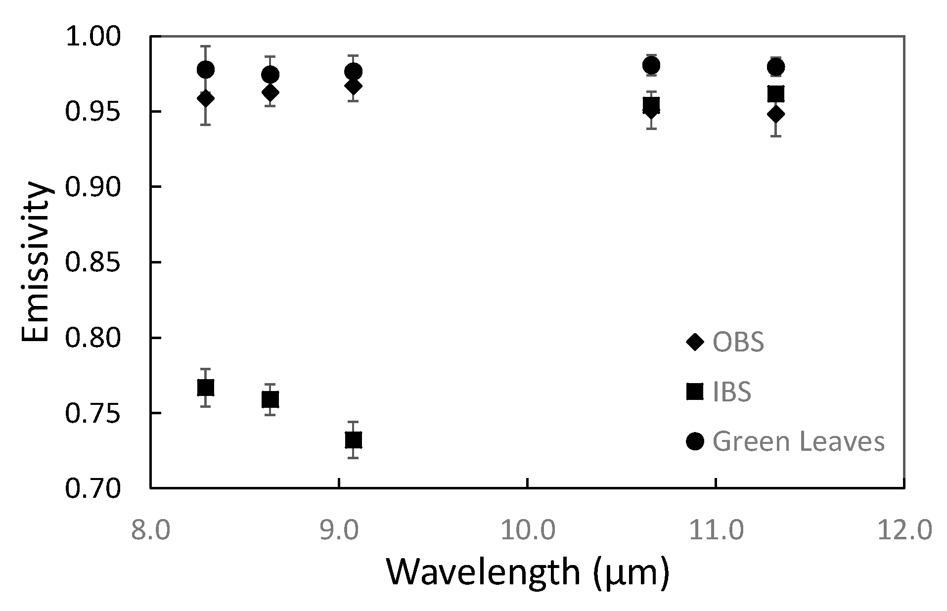
4.1. Leaf Area Index and Vegetation Cover Fraction Measurements

The LAI values required to apply the different models were obtained using Pocket-LAI App. For each LAI, obtained by cutting leaves of the rose plants used as sample, 36 pictures were taken in order to obtain the statistical values. Therefore, the value given for each LAI corresponds to the mean of these 36 pictures. These LAI values are shown in

Table 1. Leaf area index (LAI) and vegetation cover fraction (P_v) measured values required at the different models of the study to the sample with organic soil (OS) and inorganic soil (IS).

LAI (m2/m2)—OS	${\mathit{P}}_{\mathit{v}}$—OS	LAI (m2/m2)—IS	${\mathit{P}}_{\mathit{v}}$—IS
2.8 ± 0.4	0.95 ± 0.03	3.3 ± 0.5	0.98 ± 0.03
2.4 ± 0.4	0.90 ± 0.03	2.8 ± 0.3	0.96 ± 0.04
2.0 ± 0.3	0.83 ± 0.06	2.4 ± 0.3	0.91 ± 0.05
1.5 ± 0.2	0.77 ± 0.05	1.8 ± 0.3	0.81 ± 0.05
0.9 ± 0.2	0.57 ± 0.06	1.1 ± 0.2	0.62 ± 0.03
0.52 ± 0.12	0.41 ± 0.04	0.64 ± 0.07	0.44 ± 0.03

. Also, the uncertainty for each value is given. This uncertainty is calculated by the standard deviation of the 36 measurements.

In order to calculate the $P_v$ needed for Rmod3 model, six pictures were taken of the rose plants, covering the study sample uniformly, for each LAI. Then, the pixels corresponding to vegetation were distinguished by means of the selection of green pixels using image editing software. Finally, the $P_v$ of each picture was obtained by dividing the quantity of green pixels by the total number of pixels. The results of the mean $P_v$ value of the six pictures for each LAI, and its uncertainty obtained as the standard deviation, are also shown in Table 1.

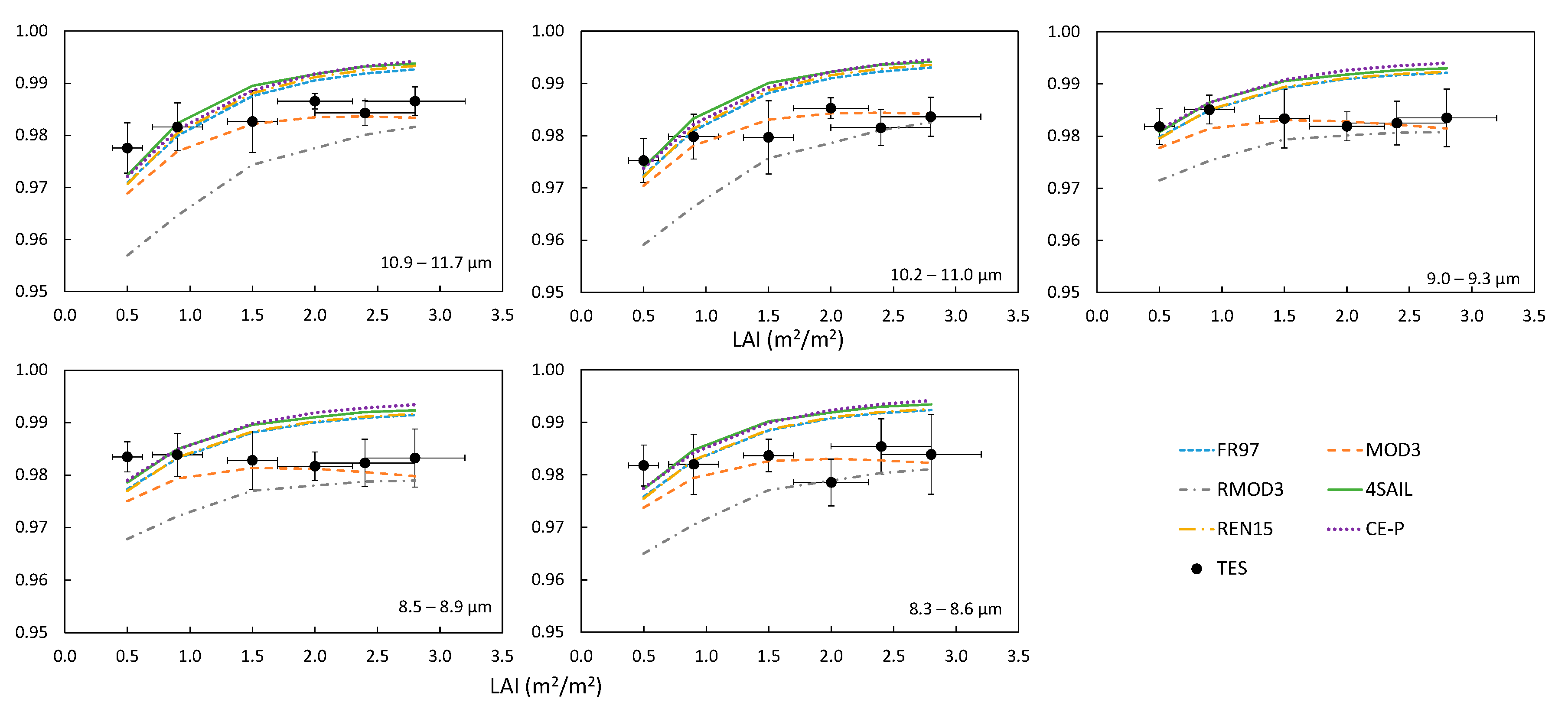
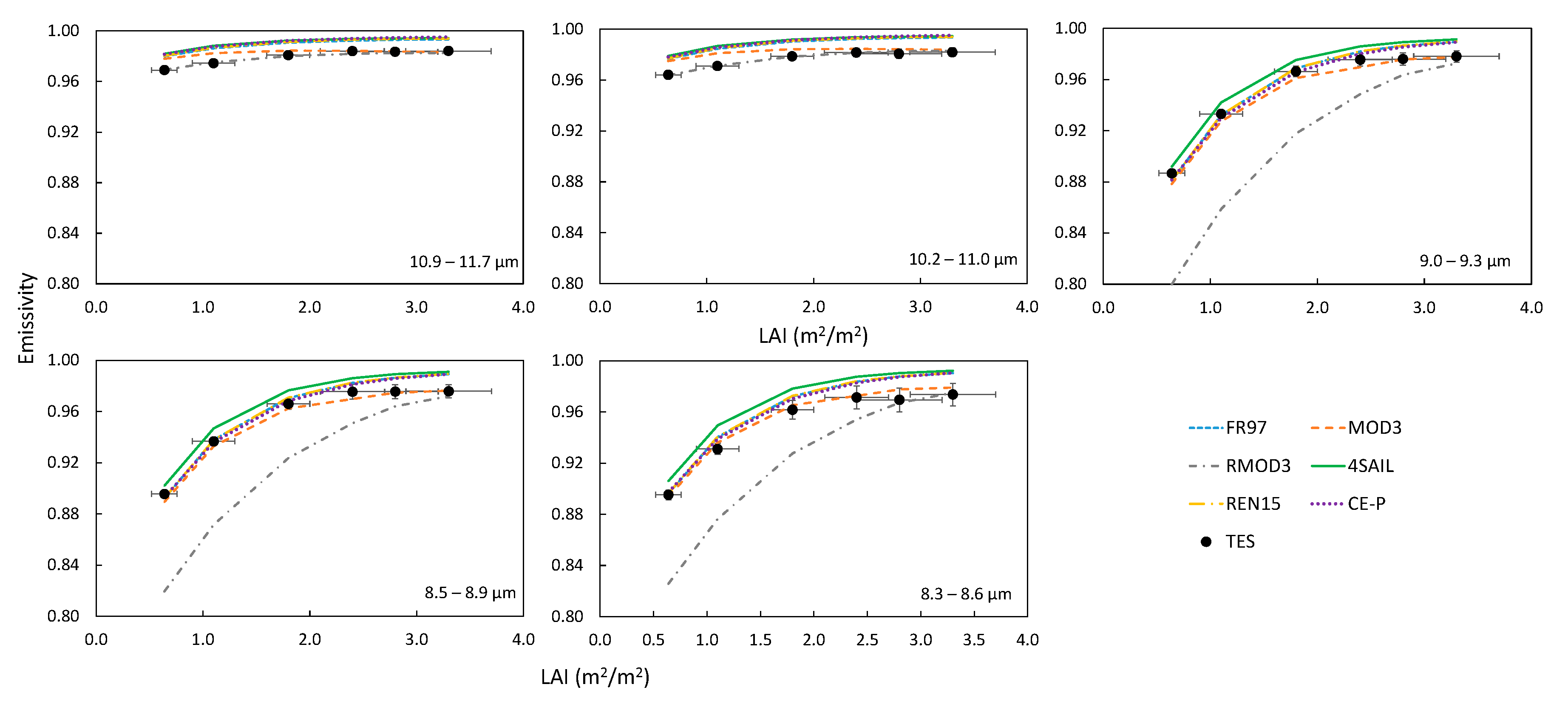
4.2. Canopy Emissivity Variation with LAI at Nadir

The emissivities measured in situ with TES algorithm at nadir are compared in Figure 3 with those emissivities given by the six RTM for the different LAI quantities in the case of the organic soil. Figure 3 is composed of five graphs, each one corresponding to a spectral narrow band of the CE312-2 radiometer.

From Figure 3, it is observed that TES emissivity values range from 0.975 to 0.987. The lower values were found for LAI of 0.5 m²/m² and in 10.2–11.0 µm, whereas the higher value was obtained for LAI of 2.8 m²/m² in 10.9–11.7 µm. Also, the uncertainties observed for emissivity range from ±0.002 to ±0.008, whereas LAI uncertainties are those of Table 1.

Figure 4 shows the at nadir emissivity obtained from TES measurements and the emissivity estimated from the RTM for the case of the inorganic soil. In Figure 4, TES emissivity values range from 0.887 obtained for 9.0–9.3 µm to 0.984 obtained for 10.9–11.7 µm. The uncertainties found for each emissivity value range from ±0.002 to ±0.009, while LAI uncertainties are those in Table 1. The spectral range of 10–12 µm shows less variation with LAI (around 0.02) because of the soil emissivity is closer to the vegetation emissivity. However, the low emissivity of sand for 8–9.5 µm range causes a high variation in the emissivity with LAI. This variation has a higher slope for LAI < 2 m²/m², where the difference of LAI has a major effect on emissivity. For LAI > 2 m²/m², the emissivity trends to plateau, taking values close to the ${\epsilon }_{lim}$.

Because of the spectral variation of sand emissivity, the higher differences between the models and the TES emissivity were found for 8–9.5 µm range in Figure 4. While for 10–12 µm of the inorganic soil measurements, we found similar results to those obtained for the organic soil, because of the similar soil emissivity. In the latter case, FR97, 4SAIL, REN15, and CE-P gave similar results, with differences lower than 0.002 between them. However, these differences are up to 0.01 for the lower LAIs when the difference between soil and leaf emissivity increase (8–9.5 µm range), but they are reduced when the LAI increase. Mod3 model gives similar values to FR97 model for low LAIs, with a difference around 0.002, but they differ with LAI, giving differences up to 0.013, with similar differences for both soils. In the case of Rmod3 model, differences with the Mod3 model decrease with LAI, varying from 0.012 to 0.001 in the case of the organic soil and 10–12 µm range of the inorganic soil. But these differences range from 0.078 to 0.004 in the case of 8–9.5 µm with the inorganic soil, when the soil and leaf emissivity differs more.

The six models were compared with at-nadir TES emissivity. The statistical results are summarized in

Table 2. Statistical values from the at-nadir comparison of the canopy emissivity models and TES algorithm for the different LAI measurements and for all bands with the organic soil.

LAI	FR97		MOD3		RMOD3		4SAIL		REN15		CE-P
	bias	RMSE	bias	RMSE	bias	RMSE	bias	RMSE	bias	RMSE	bias	RMSE
0.5	−0.005	0.005	−0.007	0.007	−0.016	0.016	−0.003	0.004	−0.005	0.005	−0.003	0.004
0.9	−0.0001	0.0012	−0.003	0.004	−0.013	0.013	0.0019	0.002	0.0001	0.0011	0.0013	0.0017
1.5	0.006	0.006	0.000	0.002	−0.006	0.006	0.008	0.008	0.006	0.006	0.007	0.007
2	0.008	0.008	0.000	0.003	−0.004	0.006	0.009	0.009	0.008	0.009	0.009	0.010
2.4	0.008	0.009	−0.001	0.002	−0.003	0.004	0.010	0.010	0.009	0.009	0.010	0.010
2.8	0.008	0.008	−0.0019	0.003	−0.003	0.004	0.009	0.009	0.009	0.009	0.010	0.010
Overall	0.004	0.007	−0.002	0.004	−0.007	0.009	0.006	0.008	0.004	0.007	0.006	0.008

and

Table 3. Statistical values from the at-nadir comparison of the canopy emissivity models and TES algorithm for the different LAI measurements and for all bands with the inorganic soil.

LAI	FR97		MOD3		RMOD3		4SAIL		REN15		CE-P
	bias	RMSE	bias	RMSE	bias	RMSE	bias	RMSE	bias	RMSE	bias	RMSE
0.64	0.003	0.009	0.001	0.009	−0.047	0.063	0.010	0.011	0.003	0.009	0.004	0.010
1.1	0.007	0.010	0.003	0.008	−0.039	0.053	0.013	0.014	0.007	0.010	0.006	0.010
1.8	0.008	0.009	0.001	0.005	−0.025	0.034	0.012	0.012	0.008	0.009	0.007	0.009
2.4	0.009	0.009	−0.001	0.004	−0.014	0.019	0.012	0.012	0.009	0.010	0.009	0.009
2.8	0.012	0.013	0.002	0.004	−0.005	0.008	0.014	0.015	0.013	0.013	0.012	0.013
3.3	0.012	0.013	0.001	0.003	−0.002	0.003	0.014	0.014	0.013	0.013	0.013	0.013
Overall	0.009	0.010	0.001	0.005	−0.022	0.036	0.013	0.013	0.010	0.011	0.009	0.011

for the different LAI values. For the organic soil, differences between models with TES emissivity were lower. It is observed in Table 2 that, for LAI < 1.5 m²/m², FR97, 4SAIL, REN15, and CE-P are the models with lower RMSE. However, for LAIs ≥ 1.5 m²/m², Mod3 model shows the lowest RMSE. Also, the RMSE for Rmod3 model decreases with LAI, because of the soil term is reduced and the values are closer to the Mod3 model. In the overall analyses, where all LAIs and spectral bands are included, Mod3 model has the lowest bias and RMSE, but the values are close to the other models, with differences in RMSE lower than 0.005. Nevertheless, for the case of inorganic soil (Table 3) the Mod3 model gives the lowest RMSE for all LAIs, although for the lowest LAI (LAI = 0.64 m²/m²) the results are the same as those obtained with FR97 and REN15 models. 4SAIL RMSE values are slightly higher than those given by the FR97, REN15, and CE-P models. Moreover, despite of 10–12 µm on Figure 4 shows that Rmod3 is the closest model to the TES measurements, the emissivity of the Rmod3 model decrease considerably for 8–9.5 µm range, yielding to values far to those given by TES emissivity. This decreasing in the Rmod3 canopy emissivity is caused by the difference between the soil and leaf emissivity. In the overall analyses, as occurs with the organic soil, it is the Mod3 model which shows the lower bias and RMSE in comparison with TES emissivity. But in this case, the differences of the Mod3 RMSE with the RMSE obtained for other models are higher, from 0.005 in the case of FR97 model to 0.036 in the case of Rmod3.

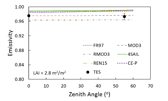
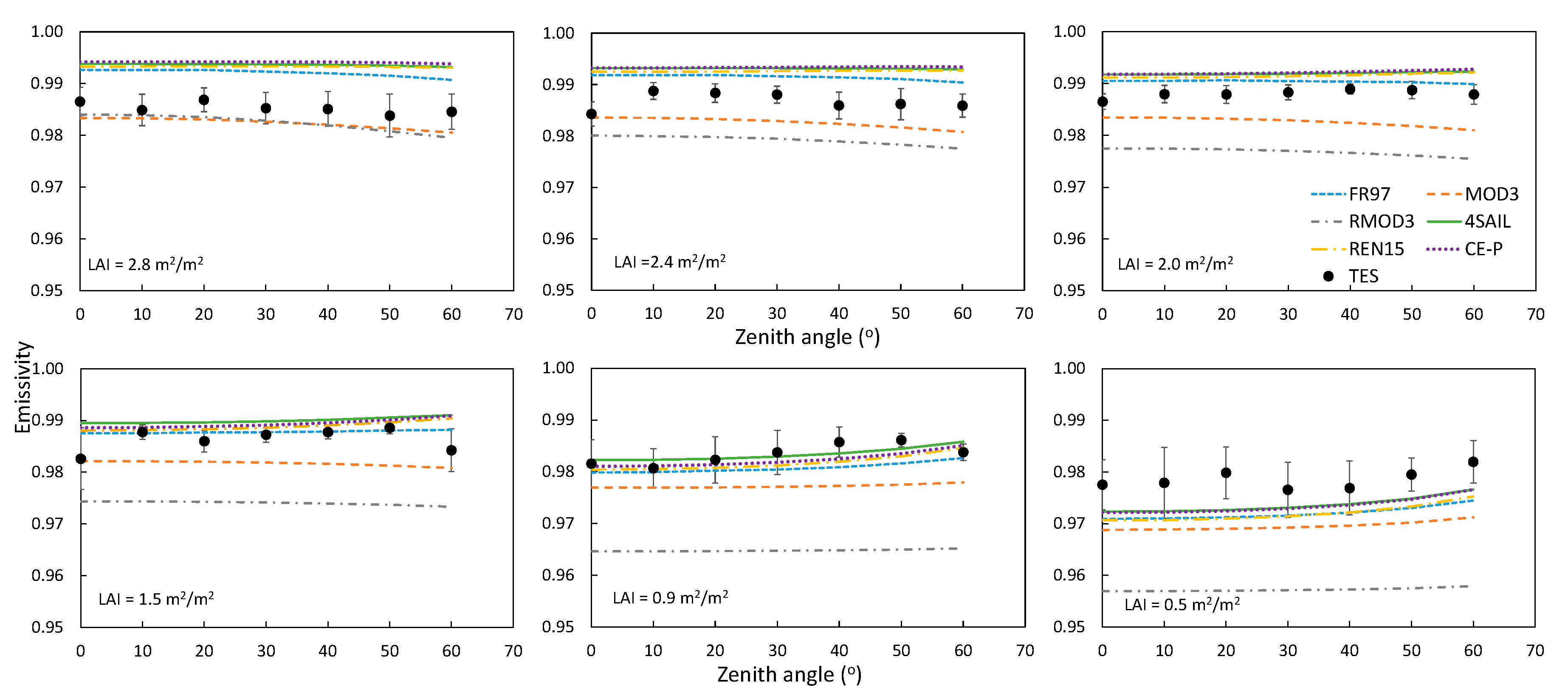
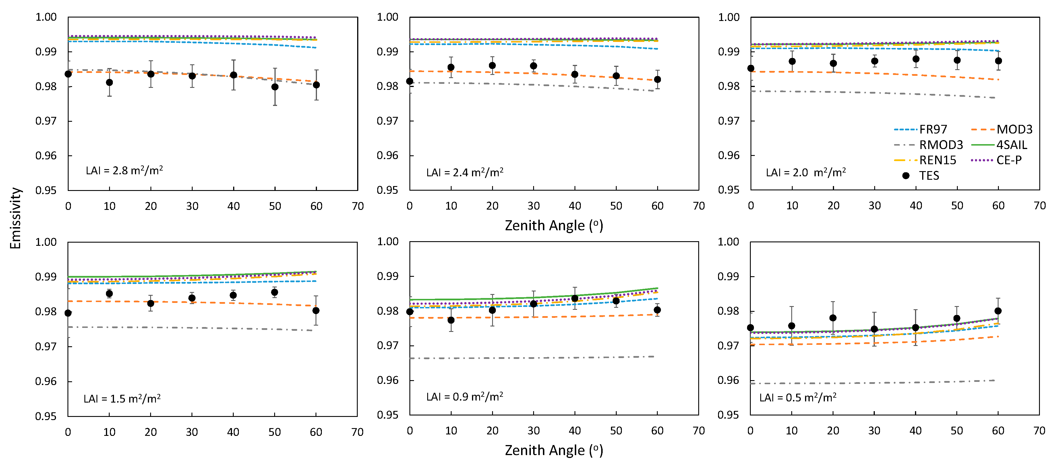
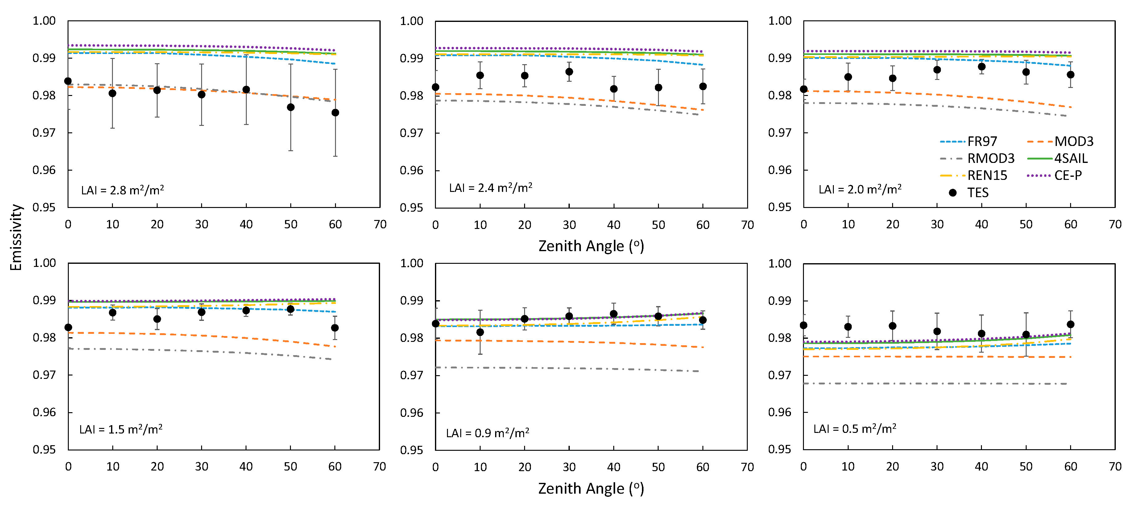
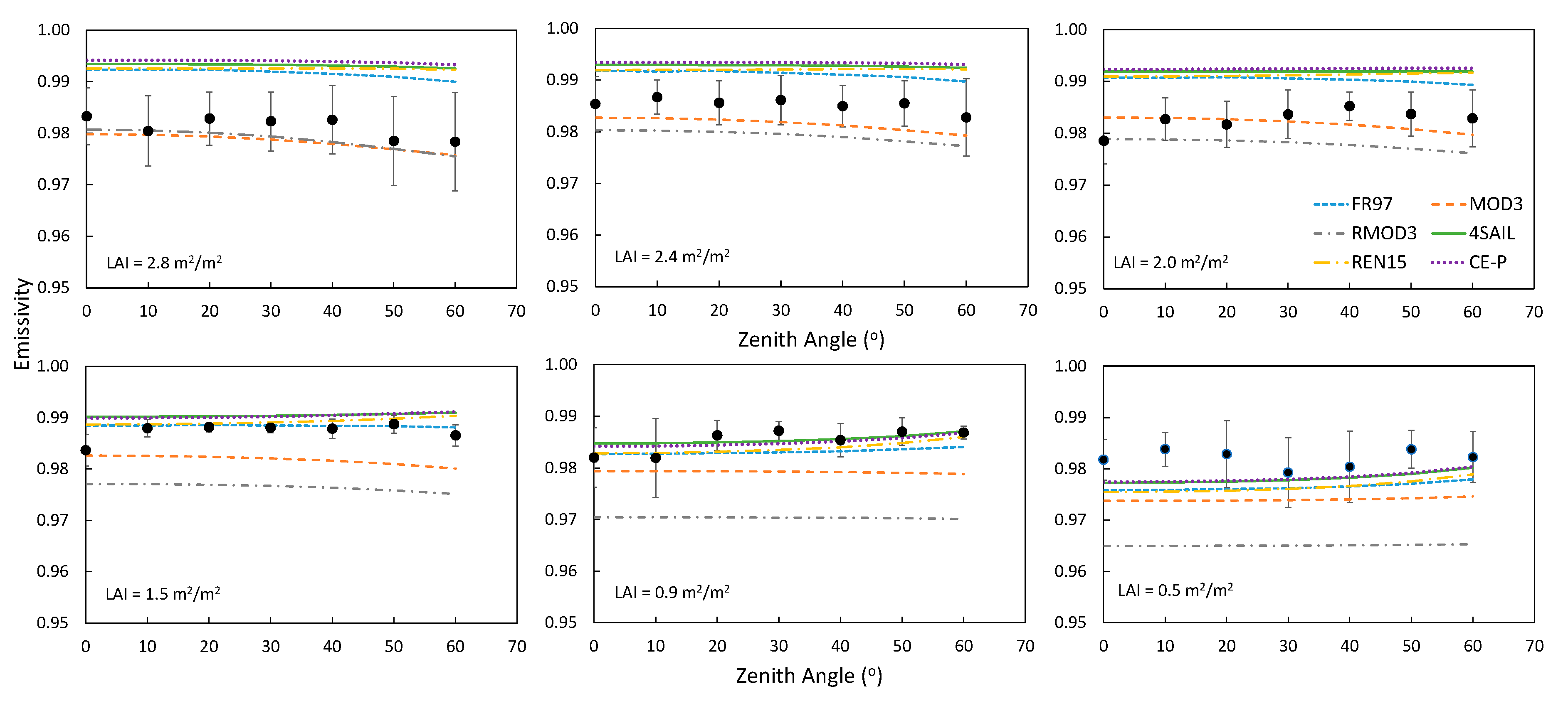
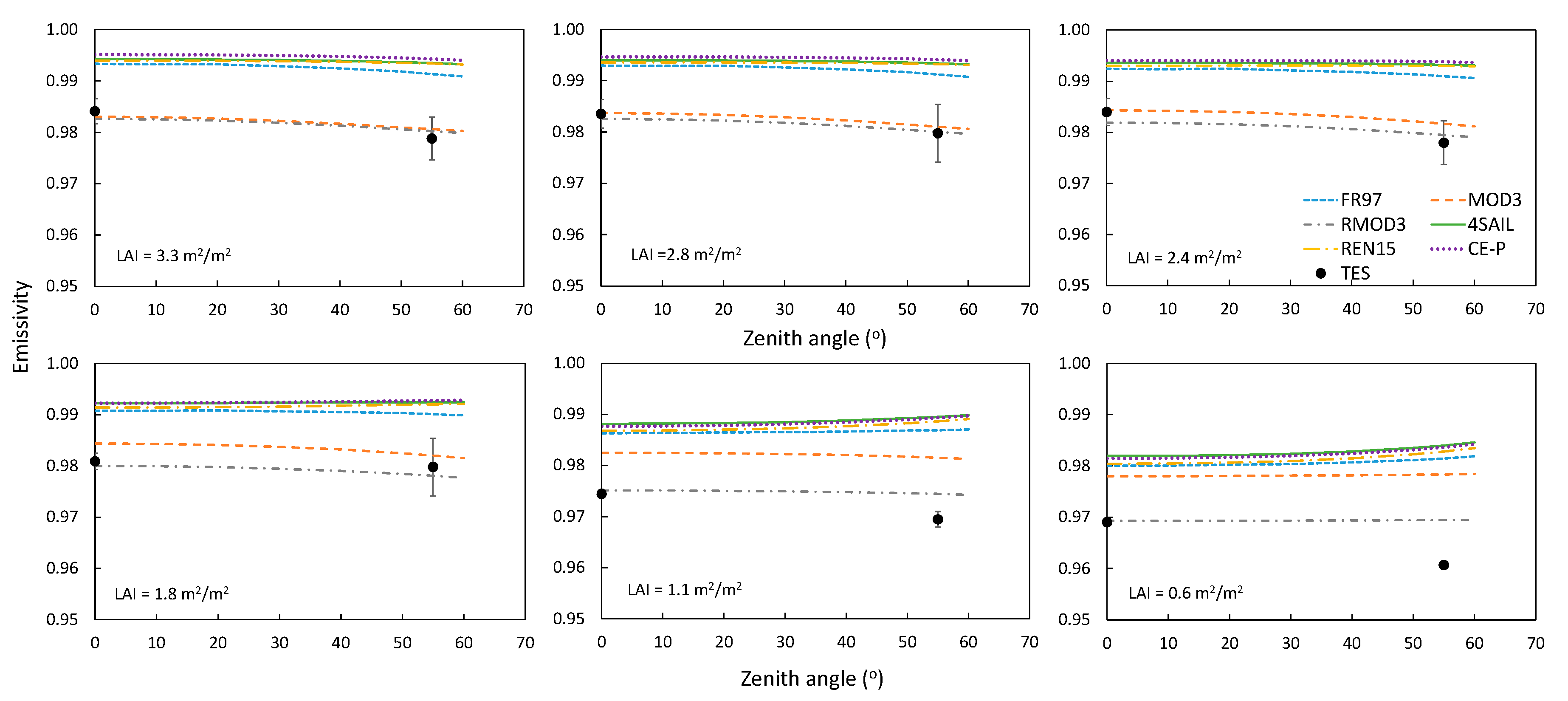
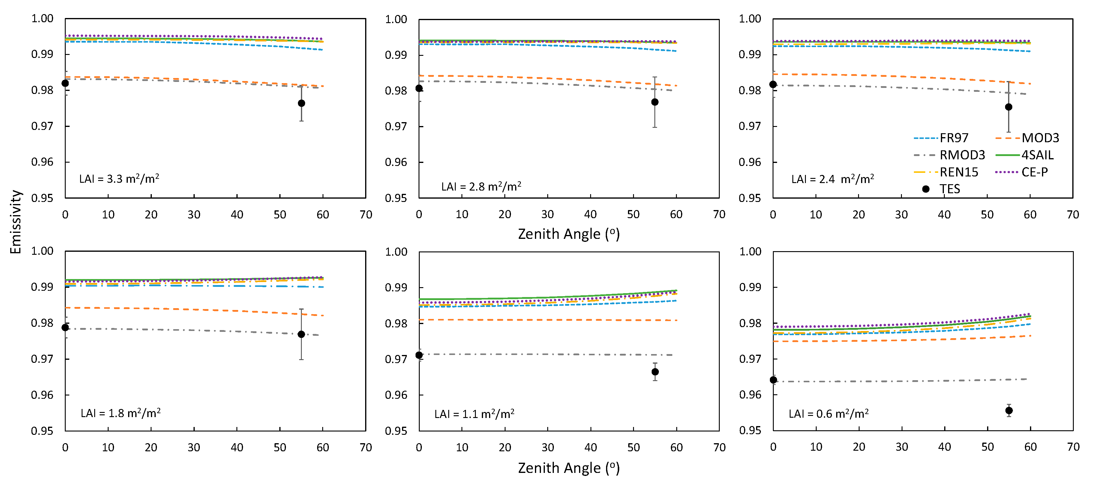
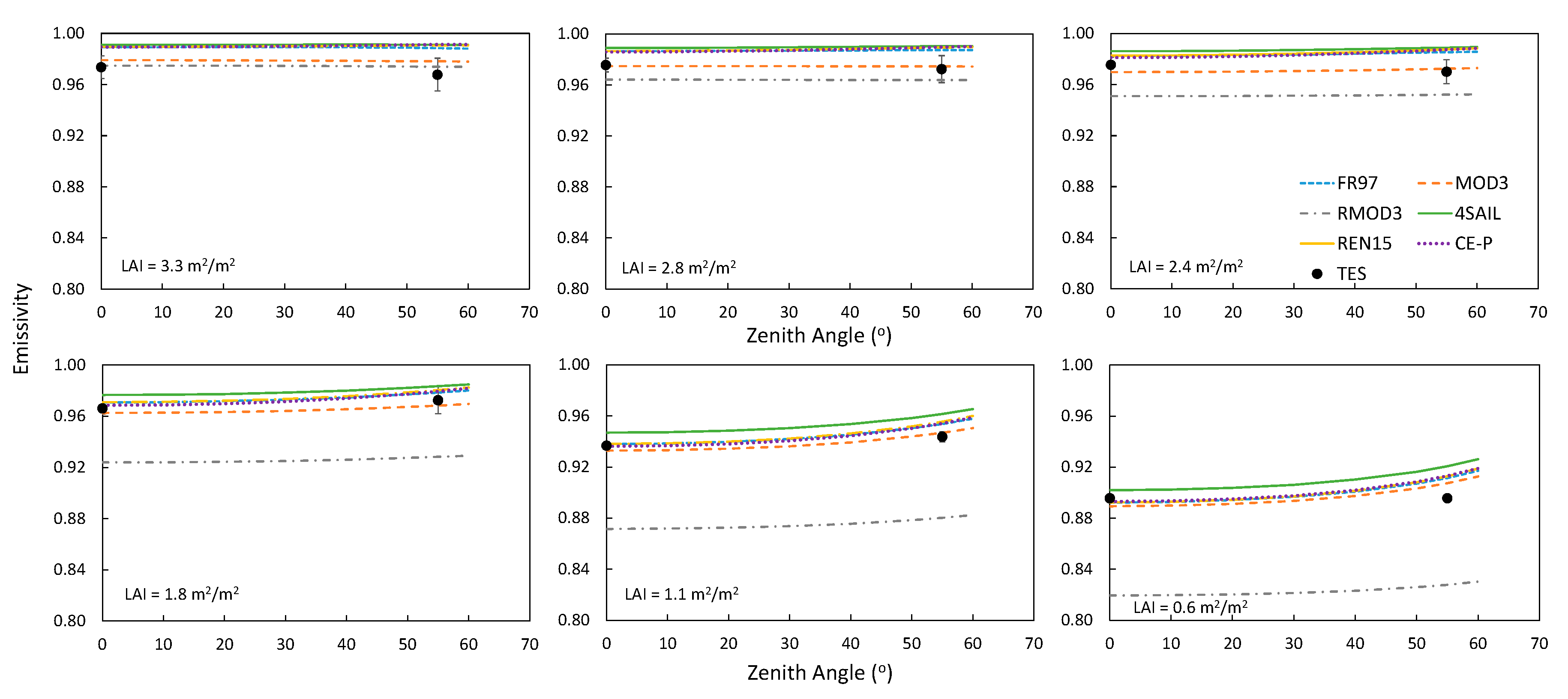
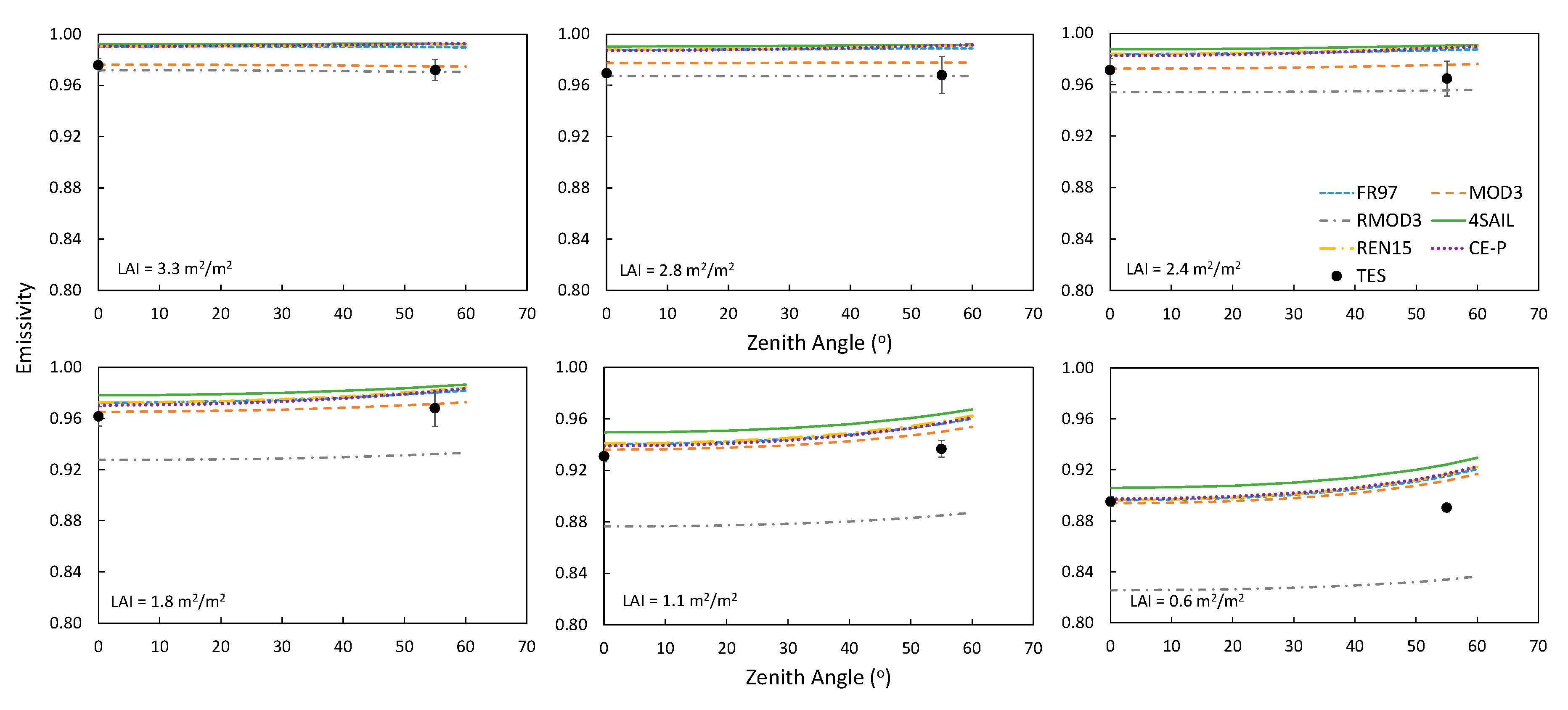
4.3. Canopy Emissivity Variation with Viewing Angle for Different LAI Values

4.3.1. Organic Soil

The six directional canopy emissivity models were also compared with the TES emissivity measured for the seven different VZAs in the case of the organic soil, from 0° to 60° in steps of 10° and for the six LAI values given in Table 1 for this soil. In Figure 5, Figure 6, Figure 7, Figure 8 and Figure 9, these comparisons are shown, each figure corresponding to one spectral narrow band of the CE312-2 radiometer. They show the emissivity given by the six models, as well as the emissivity measured by the CE312-2 radiometer with the TES algorithm.

Figure 5, Figure 6, Figure 7, Figure 8 and Figure 9 show the emissivity values obtained with TES algorithm for the 5 CE312-2 spectral bands over the rose plants and the organic soil. The obtained values ranged from 0.975 to 0.989 depending on LAI, VZA, and spectral range. The mean uncertainty, obtained as the standard deviation of the measurements, was between ±0.003 (Figure 5 and Figure 6) and ±0.005 (Figure 9).

From Figure 5, Figure 6, Figure 7, Figure 8 and Figure 9, very little variation is observed with the VZAs in the range from 0° to 60°. Also, a slight fluctuation on the TES emissivities can be observed in some figures but it is within the measurement uncertainty. As for nadir observation, 4SAIL and FR97 show a slight difference lower than 0.002, while REN15 model is closer to FR97 model for low VZAs and it takes closer values to 4SAIL model when the angle increases, as it was expected [27]. It can be observed how the differences between models are inverted when the LAI is reduced, Mod3 model is close to the FR97 model for lower LAIs (LAI < 2 m²/m²), but it is closer for Rmod3 model when LAIs are higher (LAI > 2 m²/m²), because the increment of $P_v$ makes their expressions more similar.

The relation of the models with TES emissivity seems to vary with LAI. An overestimation is observed in the FR97, 4SAIL, REN15, and CE-P models for LAIs ≥ 2.0 m²/m². However, they fit quite well for LAI < 2 m²/m². In the case of Mod3 model, it slightly underestimates the TES measurements in most cases, but no high differences are observed. Rmod3 model is the model which differs from the TES measurements. Only for high LAIs, when the values are close to those given by the Mod3 model, its values are close to the TES emissivities.

Table 4. Statistical analyses of the comparison between the canopy emissivity models and TES method at different viewing zenith angles (VZAs) for the different LAI measurements and for all bands and observation angles using the organic soil in the sample.

LAI	FR97		MOD3		RMOD3		4SAIL		REN15		CE-P
	bias	RMSE	bias	RMSE	bias	RMSE	bias	RMSE	bias	RMSE	bias	RMSE
2.8	0.010	0.010	−0.001	0.002	−0.001	0.002	0.011	0.011	0.011	0.011	0.012	0.012
2.4	0.006	0.007	−0.003	0.004	−0.006	0.006	0.008	0.008	0.007	0.008	0.009	0.009
2	0.005	0.005	−0.004	0.005	−0.008	0.008	0.006	0.007	0.006	0.006	0.007	0.007
1.5	0.003	0.004	−0.004	0.005	−0.010	0.010	0.005	0.005	0.004	0.004	0.005	0.005
0.9	−0.001	0.002	−0.005	0.006	−0.014	0.015	0.001	0.002	0.000	0.002	0.0007	0.002
0.5	−0.005	0.005	−0.007	0.007	−0.016	0.017	−0.003	0.004	−0.004	0.005	−0.003	0.003
Overall	0.003	0.006	−0.004	0.005	−0.009	0.011	0.005	0.007	0.004	0.007	0.005	0.007

summarizes the bias and RMSE of the comparison of models emissivity with TES emissivity. As it is observed from Figure 5, Figure 6, Figure 7, Figure 8 and Figure 9, the differences between TES emissivity and FR97, 4SAIL, and REN15 models increase with LAI. Contrarily, for Mod3 and Rmod3 model, the differences decrease with LAI.

4.3.2. Inorganic Soil

For the inorganic soil, the VZAs measured were 0° and 55° for the LAIs defined in Table 1 for this soil. Figure 10, Figure 11, Figure 12, Figure 13 and Figure 14 show the emissivities obtained for the five CE312-2 narrow bands from the six directional emissivity canopy models and the TES emissivity measurement for both angles. The obtained values ranged from 0.887 to 0.988 depending on LAI, VZA and spectral range. The mean uncertainty, obtained as the standard deviation of the measurements, was between ±0.003 (Figure 10) and ±0.009 (Figure 14).

From Figure 10 and Figure 11, because of the emissivity values are close to the organic soil, the models behavior is similar to that of the observed with this soil. However, differences are found in Figure 12, Figure 13 and Figure 14, where the soil emissivity is significantly lower. The differences between FR97 and 4SAIL models increase when the LAI is reduced, giving differences up to 0.01. REN15 and CE-P models remains between both, but they are always close to FR97 model for all angles. Also, the differences between Mod3 and RMod3 model increase with LAI, showing similar values for high LAIs, but the Rmod3 model decrease considerably with LAI, yielding to differences with Mod3 model up to 0.08 for the lowest LAI measured.

In the comparison with TES emissivity, FR97, 4SAIL, REN15, and CE-P models overestimate the emissivity for most cases. Opposite to the observations in the comparison of the organic soil, Rmod3 model is the model that fits better to the TES emissivity for 10–12 µm range. However, this model is largely the model that differs more with TES emissivity for 8–9.5 µm range and LAI < 2.0 m²/m², as it is shown in Figure 12, Figure 13 and Figure 14. It is Mod3 model which shows the best agreement with TES emissivity in Figure 12, Figure 13 and Figure 14, but it also gives close values for 8.3–8.9 µm and LAI > 1.5 m²/m².

Table 5. Statistical analyses of the comparison between the canopy emissivity models and TES method at different VZAs for the different LAI measurements and for all bands and observation angles using the inorganic soil in the sample.

LAI	FR97		MOD3		RMOD3		4SAIL		REN15		CE-P
	bias	RMSE	bias	RMSE	bias	bias	bias	RMSE	bias	RMSE	bias	RMSE
3.3	0.015	0.015	0.002	0.004	0.000	0.016	0.016	0.017	0.016	0.016	0.016	0.017
2.8	0.014	0.014	0.003	0.005	−0.004	0.015	0.016	0.017	0.015	0.015	0.015	0.016
2.4	0.013	0.014	0.002	0.005	−0.011	0.014	0.016	0.016	0.014	0.015	0.014	0.015
1.8	0.009	0.009	0.001	0.004	−0.026	0.010	0.013	0.013	0.010	0.011	0.009	0.010
1.1	0.011	0.013	0.006	0.009	−0.037	0.012	0.017	0.018	0.012	0.014	0.011	0.014
0.64	0.012	0.016	0.009	0.014	−0.042	0.012	0.018	0.021	0.012	0.017	0.013	0.017
Overall	0.012	0.014	0.004	0.007	−0.020	0.013	0.016	0.017	0.013	0.015	0.013	0.015

shows the bias and RMSE of the comparison of the models emissivity with TES emissivity. Taking into account all data, Mod3 model shows the best agreement with TES emissivity, with an overall RMSE of 0.007. Rmod3 model, although it shows the lowest RMSE and a null bias for LAI = 3.3 m²/m², it has largely the highest global RMSE. FR97, 4SAIL, REN15, and CE-P models obtain similar RMSE for all LAIs and total data also, obtaining a similar RMSE to Mod3 model just for the lowest LAI.

5. Discussion

Six RTM to retrieve the canopy emissivity were evaluated using in situ TES emissivity over a set of rose plants and two different soils, an organic and inorganic soil. During the time the experiment was carried out, for LAIs higher than 2.0 m²/m², the canopy was seen as an almost continuous layer of leaves. However, for LAI lower than 2.0 m²/m², the quantity of ground which was seen by the sensor increased considerably when LAI decreased (See Table 1). Therefore, for lower LAIs, it was expected to obtain higher uncertainty values, mainly because of the arbitrariness of the position of leaves causes the structure of the plant be more unpredictable, and as a consequence, it could be viewed slightly different by the sensor for each VZA. However, all the uncertainties calculated from the measurements resulted in quite similar values.

From the at nadir comparison of the emissivity models, an increase of emissivity from low to high LAI values was observed, obtaining a value close to the limit emissivity for the highest LAI. Although the limit emissivity reached with each soil is the same, since there is no effect of soil emissivity on the limit emissivity retrieval [22,27], closer values to the limit emissivity were obtained for the organic soil for LAI values lower than for the inorganic soil. Then, the soil emissivity has no impact on the canopy limit emissivity, but it does on the value of emissivity for high LAIs analyzed in this study.

When the soil emissivity is high, close to the leaf emissivity, as for the cases of the organic soil at all wavelengths and the inorganic soil at 10–12 µm, all models show differences which could be reasonable taking into account the emissivity error, since the difference values given by the different models are quite close. Despite of that, it is observed that Mod3 model provides slightly better overall results, but they cannot be conclusive, since differences are within the TES uncertainties and also depend on the LAI analyzed. But when differences between soil and leaf emissivity increase, as for 8–9.5 µm range of the inorganic soil, Mod3 is the model that best fits with TES emissivity for the data analyzed in this study. In these cases, the other models show significant discrepancies with TES emissivity. If it is just taken into account the 8–9.5 µm range of the measurements with the inorganic soil, the bias of FR97, 4SAIL, REN15, and CE-P models are 0.011, 0.017, 0.012, and 0.011, respectively, which are similar to those obtained in Table 5. Mod3 model obtains a bias of 0.002 in this case. This model differs from the FR97 model in the consideration of the multiple reflections between the leaves of the canopy. Since Mod3 model takes into account the interaction between the soil and leaves in a more adequate way, then the canopy emissivity obtained is lower than the one obtained with FR97 model; this effect is stressed in the cases where the LAI, and the quantity of leaves, is higher. It is in these cases, when the LAI is higher, in which Mod3 model shows better results than FR97 model, for both organic and inorganic soils. Rmod3 model obtained accurate results when its values were close to those given by Mod3 model, that is, when LAI is high and the contribution of soil emissivity is weak, but also for 10–12 µm range with the inorganic soil. In these cases, the same occurred for REN15, CE-P, and 4SAIL models because of a systematic difference was observed between these models and FR97 model. This is because REN15 model modifies the cavity effect of the FR97 model by using the limit emissivity values obtained from the 4SAIL model. In the case of CE-P model, despite it is based on spectral invariants as the recollision and escape probabilities instead of the cavity effect coefficient, the values obtained are quite close to those obtained by the FR97 and REN15 models. However, when the LAI decreases, and consequently the $P_v$ does, the soil emissivity gains weight and, if the soil emissivity is much lower than leaf emissivity, a strong decrease in the canopy emissivity is expected. This is why the Rmod3 model considerably decreases when LAI decreases, especially for 8–9.5 µm range measurements over the inorganic soil. In the case of the organic soil, this decrease is not so significant because of the similar values of the soil and leaf emissivity at all wavelengths.

Regarding the angular emissivity variation, a clear trend was not observed in any of the analyzed cases. The organic soil shows a decrease of emissivity with VZA (from 0 to 60°) between 0.01 and 0.02, and the inorganic soil between 0.03 and 0.06 [10]. However, models predict an increase in emissivity when LAI is reduced and more soil is seen, because of the cavity effect. TES emissivity measurements do not reflect clearly the increase or decrease with VZA. In the case of the organic soil, for LAI < 2 m²/m² and depending on the spectral range, the emissivity increases with angle with respect to the nadir between 0.001 and 0.005, which are values within the uncertainty. For the highest LAI (LAI = 2.8 m²/m²), the emissivity decreases with respect to nadir between 0.003 and 0.008, depending on the spectral range. But for high LAIs, this decreasing should be attributed to the cavity effect. For the inorganic soil, it is expected some decrease with angle; however, it is only observed for all LAIs in 10–12 µm, which are the bands with low decrease when bare soil is analyzed. These differences on the emissivity observed for the different VZAs range from 0.002 to 0.008 depending on the LAI, being higher when more soil is observed. For 8–9.5 µm range and LAI > 2 m²/m², the decrease observed is around 0.005, and also for 10.9–11.7 µm and LAI of 0.6 m²/m². But for LAIs between 1 and 2 m²/m², the emissivity increases around 0.007 with angle. Therefore, taking into account the uncertainty of the TES emissivity measurements, no significant variation of emissivity with VZAs between 0° and 60° is observed for canopy emissivity in this study.

6. Summary and Conclusions

An accurate retrieval of LST requires a precise knowledge of surface emissivity. Over vegetated areas, it is necessary to consider the multiple reflections between ground and vegetation when the canopy emissivity is calculated. Several methods to obtain the canopy emissivity are found in the literature. In this work, six RTM-based directional canopy emissivity models are evaluated with in situ TES emissivity measurements acquired with a CE312-2 radiometer. The selected models are FR97 [22], Mod3 [23], Rmod3 [26], REN15 model [27], CE-P [28], and 4SAIL model [25].

The sample used during the study was a set of rose plants with organic soil as background in the first period and with inorganic soil (sand) in a second period. Several measurements were done over the sample using a CE312-2 radiometer with five bands within 8 µm and 13 µm. We took 15 radiance measurements for each one of the seven (two) VZAs and for six LAI levels for the first (second) period. Also, the component (leaves and soil) emissivities were measured with the TES algorithm. From these emissivities, a flat spectrum was seen for the leaves, close to 0.98. For the bare soils, the obtained values were between 0.949 and 0.967 for the organic soil, and between 0.732 and 0.962 for the inorganic soil. These values were used as the input of the models for each spectral band.

We compared the model-derived and measured emissivities at nadir. For organic soil, results showed that the measured TES emissivities were similar for different LAI values. However, for inorganic soil, where the difference between soil and leaf emissivity was higher, the increase in emissivity predicted by the models is clearly reproduced by the TES measurements. The Mod3 model agreed with the TES measurements better than the other models, according to the RMSE obtained from the statistical analysis with both organic and inorganic soil, especially for bands where the difference on soil–leaf emissivity is high.

The evaluation carried out at different VZAs obtained a quite constant emissivity for both models and TES emissivity, with small variation with the VZA for both organic and inorganic soil. Thus, from this study, no variation with angle is expected for canopy emissivity in similar conditions. From the comparison among models with the TES method, for the organic soil, where the difference of soil–leaf emissivity is little, Mod3 obtained a slightly lower overall RMSE compared with FR97, REN15, CE-P, and 4SAIL, but the differences between them were within the measurement uncertainties. In addition, the model which adjusted best with the reference measurements depended on the LAI range, being the Mod3 model which provided best results for LAI > 2.0 m²/m² and the FR97 model when LAI < 2.0 m²/m². However, when the difference soil–leaf emissivity is high, as for 8–9.5 µm range of the inorganic soil, the Mod3 model gave the best results compared with TES emissivity measurements, while the FR97, REN15, CE-P, and 4SAIL models overestimated considerably the TES measurements and Rmod3 largely underestimated the TES emissivity, especially for low LAI values.

References

1. Anderson, M.C.; Kustas, W.P.; Norman, J.M.; Hain, C.R.; Mecikalski, J.R.; Schultz, L.; González-Dugo, M.P.; Cammalleri, C.; D’Urso, G.; Pimstein, A. Mapping daily evapotranspiration at field to continental scales using geostationary and polar orbiting satellite imagery. Hydrol. Earth Syst. Sci. 2011, 15, 223–239. [Google Scholar] [CrossRef] [Green Version]
2. Sánchez, J.M.; López-Urrea, R.; Rubio, E.; González-Piqueras, J.; Caselles, V. Assessing crop coefficients of sunflower and canola using two-source energy balance and thermal radiometry. Agric. Water Manag. 2014, 137, 23–29. [Google Scholar] [CrossRef]
3. Li, Z.; Tang, B.; Wu, H.; Ren, H.; Yan, G.; Wan, Z.; Trigo, I.F.; Sobrino, J.A. Satellite-derived land Surface temperature: Current status and perspectives. Remote Sens. Environ. 2013, 131, 14–37. [Google Scholar] [CrossRef] [Green Version]
4. Salisbury, J.W.; D’Aria, M. Emissivity of terrestrial materials in the 8–14 μm atmospheric window. Remote Sens. Environ. 1992, 42, 83–106. [Google Scholar] [CrossRef]
5. Baldridge, A.M.; Hook, S.J.; Grove, C.I.; Rivera, G. The ASTER spectral library version 2.0. Remote Sens. Environ. 2009, 113, 711–715. [Google Scholar] [CrossRef]
6. Ullah, S.; Schlerf, M.; Skidmore, A.K.; Hecker, C. Identifying plant species using mid-wave infrared (2.5–6 μm) and thermal infrared (8–14 μm) emissivity spectra. Remote Sens. Environ. 2012, 118, 95–102. [Google Scholar] [CrossRef]
7. Rock, G.; Gerhards, M.; Schlerf, M.; Hecker, C.; Udelhoven, T. Plant species discrimination using emissive thermal infrared imaging spectroscopy. Int. J. Appl. Earth Obs. Geoinf. 2016, 53, 16–26. [Google Scholar] [CrossRef]
8. Labed, J.; Stoll, M.P. Angular variation of land surface spectral emissivity in the thermal infrared: Laboratory investigations on bare soils. Int. J. Remote Sens. 1992, 12, 2299–2310. [Google Scholar] [CrossRef]
9. Cuenca, J.; Sobrino, J.A. Experimental measurements for studying angular and spectral variation of thermal infrared emissivity. Appl. Opt. 2004, 43, 4598–4602. [Google Scholar] [CrossRef]
10. García-Santos, V.; Valor, E.; Caselles, V.; Burgos, M.A.; Coll, C. On the angular variation of thermal infrared emissivity of inorganic soils. J. Geophys. Res. 2012, 117, D19116. [Google Scholar] [CrossRef] [Green Version]
11. Salisbury, J.W.; D’Aria, M. Infrared (8–14 mm) remote sensing of soil particle size. Remote Sens. Environ. 1992, 42, 157–165. [Google Scholar] [CrossRef]
12. Mira, M.; Valor, E.; Caselles, V.; Rubio, E.; Coll, C.; Galve, J.M.; Niclos, R.; Sánchez, J.M.; Boluda, R. Soil moisture effect on thermal infrared (8–13-mm) emissivity. IEEE Trans. Geosci. Remote Sens. 2010, 48, 2251–2260. [Google Scholar] [CrossRef]
13. García-Santos, V.; Valor, E.; Caselles, V.; Coll, C.; Burgos, M.A. Effect of Soil Moisture on the Angular Variation of Thermal Infrared Emissivity of Inorganic Soils. IEEE Geosci. Remote Sens. Lett. 2014, 11, 1091–1095. [Google Scholar] [CrossRef] [Green Version]
14. Warren, S.G.; Wiscombe, W.J. A model for the spectral albedo of snow. II: Snow containing atmospheric aerosols. J. Atmos. Sci. 1980, 37, 2734–2745. [Google Scholar] [CrossRef]
15. Hapke, B. Theory of Reflectance and Emittance Spectroscopy; Cambridge Univ. Press: NewYork, NY, USA, 2012; p. 455. [Google Scholar]
16. García-Santos, V.; Valor, E.; Caselles, V.; Doña, C. Validation and comparison of two models based on the Mie theory to predict 8–14 μm emissivity spectra of mineral surfaces. J. Geophys. Res. Solid Earth 2016, 121, 1739–1757. [Google Scholar] [CrossRef] [Green Version]
17. García-Santos, V.; Valor, E.; Di Biagio, C.; Caselles, V. Predictive Power of the Emissivity Angular Variation of Soils in the Thermal Infrared (8–14 μm) Region by Two Mie-Based Emissivity Theoretical Models. IEEE Geosci. Remote Sens. Lett. 2018, 15, 1115–1119. [Google Scholar] [CrossRef]
18. Cao, B.; Liu, Q.; Du, Y.; Roujean, J.L.; Gastellu-Etchegorry, J.P.; Trigo, I.F.; Zhan, W.; Yu, Y.; Cheng, J.; Jacob, F.; et al. A review of earth surface thermal radiation directionality observing and modeling: Historical development, current status and perspectives. Remote Sens. Environ. 2019, 232, 111304. [Google Scholar] [CrossRef]
19. Snyder, W.C.; Wan, Z. BRDF models to predict spectral reflectance and emissivity in the thermal infrared. IEEE Trans. Geosci. Remote Sens. 1998, 36, 214–225. [Google Scholar] [CrossRef] [Green Version]
20. Sobrino, J.A.; Caselles, V. Thermal infrared radiance model for interpreting the directional radiometric temperature of a vegetative surface. Remote Sens. Environ. 1990, 33, 193–199. [Google Scholar] [CrossRef]
21. Valor, E.; Caselles, V. Validation of the vegetation cover method for land surface emissivity estimation. In Recent Research Developments in Thermal Remote Sensing; Research Signpost: Kerala, India, 2005. [Google Scholar]
22. François, C.; Ottlé, C.; Prévot, L. Analytical parameterization of canopy directional emissivity and directional radiance in the thermal infrared. Application on the retrieval of soil and foliage temperatures using two directional measurements. Int. J. Remote Sens. 1997, 18, 2587–2621. [Google Scholar] [CrossRef]
23. François, C. The potential of directional radiometric temperatures for monitoring soil and leaf temperature and soil moisture status. Remote Sens. Environ. 2002, 80, 122–133. [Google Scholar] [CrossRef]
24. Guillevic, P.; Gastellu-Etchegorry, J.P.; Demarty, J.; Prévot, L. Thermal infrared radiative transfer within three-dimensional vegetation covers. J. Geophys. Res. 2003, 108, 4248. [Google Scholar] [CrossRef]
25. Verhoef, W.; Jia, L.; Xiao, Q.; Su, Z. Unified Optical-Thermal Four-Stream Radiative Transfer Theory for Homogeneous Vegetation Canopies. IEEE Trans. Geosci. Remote Sens. 2007, 45, 1808–1822. [Google Scholar] [CrossRef]
26. Shi, Y. Thermal infrared inverse model for component temperatures of mixed pixels. Int. J. Remote Sens. 2011, 32, 2297–2309. [Google Scholar] [CrossRef]
27. Ren, H.; Liu, R.; Yan, G.; Li, Z.L.; Qin, Q.; Liu, Q.; Nerry, F. Performance evaluation of four directional emissivity analytical models with thermal SAIL model and airborne images. Opt. Express 2015, 23, A346–A360. [Google Scholar] [CrossRef] [PubMed]
28. Cao, B.; Guo, M.; Fan, W.; Xu, X.; Peng, J.; Ren, H.; Du, Y.; Li, H.; Bian, Z.; Hu, T.; et al. A new directional canopy emissivity model based on spectral invariants. IEEE Trans. Geosci. Remote Sens. 2018, 56, 6911–6926. [Google Scholar] [CrossRef] [Green Version]
29. Sobrino, J.A.; Jiménez-Muñoz, J.C.; Verhoef, W. Canopy directional emissivity: Comparison between models. Remote Sens. Environ. 2005, 99, 304–314. [Google Scholar] [CrossRef]
30. Neinavaz, E.; Skidmore, A.K.; Darvishzadeh, R.; Groen, T.A. Retrieval of leaf area index in different plant species using thermal hyperspectral data. ISPRS J. Photogramm. Remote Sens. 2016, 119, 390–401. [Google Scholar] [CrossRef]
31. Neinavaz, E.; Darvishzadeh, R.; Skidmore, A.K.; Groen, T.A. Measuring the response of canopy emissivity spectra to leaf area index variation using thermal hyperspectral data. Int. J. Appl. Earth Obs. Geoinf. 2016, 53, 40–47. [Google Scholar] [CrossRef]
32. Gillespie, A.; Rokugawa, S.; Matsunaga, T.; Cothern, J.S.; Hook, S.; Kahle, A.B. A Temperature and Emissivity Separation Algorithm for Advanced Spaceborne Thermal Emission and Reflection Radiometer (ASTER) Images. IEEE Trans. Geosci. Remote Sens. 1998, 36, 1113–1126. [Google Scholar] [CrossRef]
33. Coll, C.; Niclòs, R.; Puchades, J.; García-Santos, V.; Galve, J.M.; Pérez-Planells, L.; Valor, E.; Thecharous, E. Laboratory calibration and field measurement of land surface temperature and emissivity using thermal infrared multiband radiometers. Int. J. Appl. Earth Obs. Geoinf. 2019, 78, 227–239. [Google Scholar] [CrossRef]
34. Legrand, M.; Pietras, C.; Brogniez, G.; Haeffelin, M.; Abuhassan, N.K.; Sicard, M. A high-accuracy multiwavelength radiometer for in situ measurements in the thermal infrared. Part I: Characterization of the instrument. J. Atmos. Ocean. Technol. 2000, 17, 1203–1214. [Google Scholar] [CrossRef]
35. Confalonieri, R.; Foi, M.; Casa, R.; Aquaro, S.; Tona, E.; Peterle, M.; Boldini, A.; Carli, G.D.; Ferrari, A.; Finotto, G. Development of an app for estimating leaf area index using a smartphone. Trueness and precision determination and comparison with other indirect methods. Comput. Electron. Agric. 2013, 96, 67–74. [Google Scholar] [CrossRef]
36. Korb, A.R.; Dybwad, P.; Wadsworth, W.; Salisbury, J.W. Portable Fourier transform infrared spectroradiometer for field measurements of radiance and emissivity. Appl. Opt. 1996, 35, 1679–1692. [Google Scholar] [CrossRef] [PubMed] [Green Version]
37. Theocharous, E.; Fox, N.P.; Barker-Snook, I.; Niclòs, R.; García-Santos, V.; Minnett, P.; Göttsche, F.M.; Poutier, L.; Morgan, N.; Nightingale, T.; et al. The 2016 CEOS infrared radiometer comparison: Part 2: Laboratory comparison of radiation thermometers. J. Atmos. Ocean. Technol. 2019, 36, 1079–1092. [Google Scholar] [CrossRef] [Green Version]
38. García-Santos, V.; Valor, E.; Caselles, V.; Mira, M.; Galve, J.M.; Coll, C. Evaluation of different methods to retrieve the hemispherical downwelling irradiance in the thermal infrared region for field measurements. IEEE Trans. Geosci. Remote Sens. 2013, 51, 2155–2165. [Google Scholar] [CrossRef]
39. Coll, C.; Caselles, V.; Valor, E.; Niclòs, R.; Sánchez, J.M.; Galve, J.M.; Mira, M. Temperature and emissivity separation from ASTER data for low spectral contrast surfaces. Remote Sens. Environ. 2007, 110, 162–175. [Google Scholar] [CrossRef]
40. Gillespie, A.R.; Abbott, E.A.; Gilson, L.; Hulley, G.; Jiménez-Muñoz, J.C.; Sobrino, J.A. Residual errors in ASTER temperature and emissivity standard products AST08 and AST05. Remote Sens. Environ. 2011, 115, 3681–3694. [Google Scholar] [CrossRef]
41. Pérez-Planells, L.; Valor, E.; Coll, C.; Niclòs, R. Comparison and Evaluation of the TES and ANEM Algorithms for Land Surface Temperature and Emissivity Separation over the Area of Valencia, Spain. Remote Sens. 2017, 9, 1251. [Google Scholar] [CrossRef] [Green Version]
42. Mira, M.; Schmugge, T.J.; Valor, E.; Caselles, V.; Coll, C. Comparison of thermal emissivities retrieved with the two-lid box and TES methods with laboratory spectra. IEEE Trans. Geosci. Remote Sens. 2009, 47, 1012–1021. [Google Scholar] [CrossRef]
43. Gillespie, A. Lithologic Mapping of Silicate Rocks Using TIMS; TIMS Data User’sWorkshop Jet Propulsion Laboratory: Pasadena, CA, USA, 1986; pp. 29–44. [Google Scholar]
44. Hulley, G.; Hook, S.J. The North American ASTER Land Surface Emissivity Database (NAALSED) Version 2.0. Remote Sens. Environ. 2009, 113, 1967–1975. [Google Scholar] [CrossRef]
45. Chen, J.M.; Black, T.A. Defining leaf area index for non-flat leaves. Plant Cell Environ. 1992, 15, 421–429. [Google Scholar] [CrossRef]
46. Baret, F.; De Solan, B.; Lopez-Lozano, R.; Ma, K.; Weiss, M. GAI estimates of row crops from downward looking digital photos taken perpendicular to rows at 57.5 zenith angle: Theoretical considerations based on 3D architecture models and application to wheat crops. Agric. For. Meteorol. 2010, 150, 1393–1401. [Google Scholar] [CrossRef]
47. Campos-Taberner, M.; García-Haro, F.J.; Confalonieri, R.; Martínez, B.; Moreno, Á.; Sánchez-Ruiz, S.; Gilabert, M.A.; Camacho, F.; Boschetti, M.; Busetto, L. Multitemporal Monitoring of Plant Area Index in the Valencia Rice District with PocketLAI. Remote Sens. 2016, 8, 202. [Google Scholar] [CrossRef] [Green Version]
48. Francone, C.; Pagani, V.; Foi, M.; Cappelli, G.; Confalonieri, R. Comparison of leaf area index estimates by ceptometer and PocketLAI smart app in canopies with different structures. Field Crop. Res. 2014, 155, 38–41. [Google Scholar] [CrossRef]
49. Orlando, F.; Movedi, E.; Coduto, D.; Parisi, S.; Brancadoro, L.; Pagani, V.; Guarneri, T.; Confalonieri, R. Estimating Leaf Area Index (LAI) in Vineyards Using the PocketLAI Smart-App. Sensors 2016, 16, 2004. [Google Scholar] [CrossRef] [PubMed] [Green Version]
50. Orlando, F.; Movedi, E.; Paleari, L.; Gilardelli, C.; Foi, M.; Dell’Oro, M.; Confalonieri, R.; Hermy, M. Estimating leaf area index in tree species using the PocketLAI smart app. Appl. Veg. Sci. 2015, 18, 716–723. [Google Scholar] [CrossRef]
51. Prévot, L. Modélisation des Échanges radiatifs au Sein des Couverts Végétaux. Application à la Télédétection. Validation sur un Couvert de Maïs. Ph.D. Thesis, University of Paris VI, Paris, France, 1985. [Google Scholar]
52. Chehbouni, A.; Nouvellon, Y.; Kerr, Y.H.; Moran, M.S.; Watts, C.; Prévot, L.; Watts, C.; Goodrich, D.C.; Rambal, S. Directional effect on radiative surface temperature measurements over a semi-arid grassland site. Remote Sens. Environ. 2001, 76, 360–372. [Google Scholar] [CrossRef]
53. Verhoef, W. Light scattering by leaf layers with application to canopy reflectance modeling: The SAIL model. Remote Sens. Environ. 1984, 16, 125–141. [Google Scholar] [CrossRef] [Green Version]
54. Guo, M.; Cao, B.; Fan, W.; Ren, H.; Cui, Y.; Du, Y.; Liu, Q. Scattering effect contributions to the directional canopy emissivity and brightness temperature based on CE-P and CBT-P models. IEEE Geosci. Remote Sens. Lett. 2019, 16, 957–961. [Google Scholar] [CrossRef]
Figure 1. Experimental setup established for the radiometric measurements.
Remotesensing 11 03011 g001
Figure 2. Band emissivity of green leaves, organic bare soil (OBS) and inorganic bare soil (IBS) measured in situ with the temperature-emissivity separation (TES) algorithm.
Remotesensing 11 03011 g002
Figure 3. TES in situ nadir emissivity and emissivity values given by FR97, Mod3, Rmod3, REN15, CE-P, and 4SAIL models for nadir observation for different LAIs over the organic soil.
Remotesensing 11 03011 g003
Figure 4. TES in situ nadir emissivity and emissivity values given by FR97, Mod3, Rmod3, REN15, CE-P, and 4SAIL models for nadir observation for different LAIs over the inorganic soil.
Remotesensing 11 03011 g004
Figure 5. TES emissivity measurements and FR97, Mod3, Rmod3, 4SAIL, REN15, and CE-P models emissivity values at different zenith angles and LAI values for the CE312-2 radiometer 10.9–11.7 spectral band using an organic soil.
Remotesensing 11 03011 g005
Figure 6. TES emissivity measurements and FR97, Mod3, Rmod3, 4SAIL, REN15, and CE-P models emissivity values at different zenith angles and LAI values for the CE312-2 radiometer 10.2–11.0 µm spectral band using an organic bare soil.
Remotesensing 11 03011 g006
Figure 7. TES emissivity measurements and FR97, Mod3, Rmod3, 4SAIL, REN15, and CE-P models emissivity values at different zenith angles and LAI values for the CE312-2 radiometer 9.0–9.3 µm spectral band using an organic soil.
Remotesensing 11 03011 g007
Figure 8. TES emissivity measurements, and FR97, Mod3, Rmod3, 4SAIL, REN15, and CE-P models emissivity values at different zenith angles and LAI values for the CE312-2 radiometer 8.5–8.9 µm spectral band using and organic soil.
Remotesensing 11 03011 g008
Figure 9. TES emissivity measurements and FR97, Mod3, Rmod3, 4SAIL, REN15, and CE-P models emissivity at different zenith angles and LAI values for the CE312-2 radiometer 8.3–8.6 µm spectral band using an organic soil.
Remotesensing 11 03011 g009
Figure 10. TES emissivity measurements and FR97, Mod3, Rmod3, 4SAIL, REN15, and CE-P models emissivity values at different zenith angles and LAI values for the CE312-2 radiometer 10.9–11.7 µm spectral band using an inorganic soil.
Remotesensing 11 03011 g010
Figure 11. TES emissivity measurements and FR97, Mod3, Rmod3, 4SAIL, REN15, and CE-P models emissivity values at different zenith angles and LAI values for the CE312-2 radiometer 10.2–11.0 µm spectral band using an inorganic bare soil.
Remotesensing 11 03011 g011
Figure 12. TES emissivity measurements and FR97, Mod3, Rmod3, 4SAIL, REN15, and CE-P models emissivity values at different zenith angles and LAI values for the CE312-2 radiometer 9.0–9.3 µm spectral band using an inorganic soil.
Remotesensing 11 03011 g012
Figure 13. TES emissivity measurements, and FR97, Mod3, Rmod3, 4SAIL, REN15, and CE-P models emissivity values at different zenith angles and LAI values for the CE312-2 radiometer 8.5–8.9 µm spectral band using an inorganic soil.
Remotesensing 11 03011 g013
Figure 14. TES emissivity measurements, and FR97, Mod3, Rmod3, 4SAIL, REN15, and CE-P models emissivity values at different zenith angles and LAI values for the CE312-2 radiometer 8.3–8.6 µm spectral band using an inorganic soil.
Remotesensing 11 03011 g014