Article

Spatial Modeling of Snow Avalanche Using Machine Learning Models and Geo-Environmental Factors: Comparison of Effectiveness in Two Mountain Regions

1
Geographic Information Science Research Group, Ton Duc Thang University, Ho Chi Minh City 70000, Vietnam
2
Faculty of Environment and Labour Safety, Ton Duc Thang University, Ho Chi Minh City 70000, Vietnam
3
Department of Geoinformatics—Z_GIS, University of Salzburg, 5020 Salzburg, Austria
4
Faculty of Natural Resources, University of Tehran, Karaj 31587-77871, Iran
5
Department of Geography, Texas State University, San Marcos, TX 78666, USA
6
Department of Watershed Management, Faculty of Natural Resources and Agriculture, Lorestan University, Khorramabad 68151-44316, Iran
7
Department of Surveying and Geoinformatics, Faculty of Geosciences and Environmental Engineering, Southwest Jiaotong University, Xipu Campus, Chengdu 611756, China
8
Institute of Research and Development, Duy Tan University, Da Nang 550000, Vietnam
9
GIS Group, Department of Business and IT, University of South-Eastern Norway, Gullbringvegen 36, N-3800 Bø i Telemark, Norway
*
Authors to whom correspondence should be addressed.
Remote Sens. 2019, 11(24), 2995; https://doi.org/10.3390/rs11242995
Submission received: 31 October 2019 / Revised: 1 December 2019 / Accepted: 7 December 2019 / Published: 13 December 2019

Abstract

:
Although snow avalanches are among the most destructive natural disasters, and result in losses of life and economic damages in mountainous regions, far too little attention has been paid to the prediction of the snow avalanche hazard using advanced machine learning (ML) models. In this study, the applicability and efficiency of four ML models: support vector machine (SVM), random forest (RF), naïve Bayes (NB) and generalized additive model (GAM), for snow avalanche hazard mapping, were evaluated. Fourteen geomorphometric, topographic and hydrologic factors were selected as predictor variables in the modeling. This study was conducted in the Darvan and Zarrinehroud watersheds of Iran. The goodness-of-fit and predictive performance of the models was evaluated using two statistical measures: the area under the receiver operating characteristic curve (AUROC) and the true skill statistic (TSS). Finally, an ensemble model was developed based upon the results of the individual models. Results show that, among individual models, RF was best, performing well in both the Darvan (AUROC = 0.964, TSS = 0.862) and Zarrinehroud (AUROC = 0.956, TSS = 0.881) watersheds. The accuracy of the ensemble model was slightly better than all individual models for generating the snow avalanche hazard map, as validation analyses showed an AUROC = 0.966 and a TSS = 0.865 in the Darvan watershed, and an AUROC value of 0.958 and a TSS value of 0.877 for the Zarrinehroud watershed. The results indicate that slope length, lithology and relative slope position (RSP) are the most important factors controlling snow avalanche distribution. The methodology developed in this study can improve risk-based decision making, increases the credibility and reliability of snow avalanche hazard predictions and can provide critical information for hazard managers.

Graphical Abstract

1. Introduction

One of the most dangerous hazards in mountainous regions is the snow avalanche. These events can greatly impact individual users of mountain environments, residential areas in avalanche zones, ecosystems, and public infrastructure [1,2,3]. From a geomorphological viewpoint, snow avalanches can produce a range of different erosional and depositional landforms (also termed as snow avalanche impact landforms) which have been well-documented [4,5,6]. Also, snow avalanches play a vital role in sedimentary mass transfer [7,8]. New constructions of roads and highways and the expansion of urbanization in mountainous areas have led to an increase in avalanche hazard [9]. Therefore, predicting the zones of this hazard is essential for the reduction of risk (the probability of avalanche occurrence) and for the mitigation of avalanche hazards (the probability of impacts on people and their interests) [10,11]. Different approaches have been employed for producing a snow avalanche susceptibility map (SASM), including multi-criteria decision analysis (MCDA) methods [12,13,14] and fuzzy-frequency ratio models [15,16,17]. However, these methods are expert opinion-based and subjective. Some researchers have used numerical methods and dynamic models to analyze the snow avalanche hazard [18,19,20,21], however a lot of uncertainty is involved in all the modeling parameters when applying to large regions at smaller scales. Other research methods are based upon remote-sensing techniques [14,22,23,24,25]. Though remote sensing can provide useful information about snow surface and land surface conditions, analysis of the complicated relationships between snow avalanches and geomorphometrics has been often ignored.
Machine learning techniques have contributed significantly to studies of numerous natural hazards, such as landslides [26,27,28,29,30], floods [31,32,33,34,35,36], gully erosion [37,38,39,40], land subsidence [41,42,43,44,45] and debris flows [46,47,48].
In the case of snow avalanches, to the best of our knowledge, too little attention has been paid to the use of machine learning models for mapping. Little is known about the efficiency of these models, and it is not clear which geomorphometric and topohydrological factors affect snow avalanche distribution and activity. Recently, Kumar et al. [49] used a simple data-mining method, probabilistic occurrence ratio (POR) (also known as a frequency ratio), and a snow avalanche inventory to prepare a snow avalanche hazard map in the Lahaul region of the western Himalayas. Their results indicated that this simple model performed well in the task of identifying snow avalanche-prone areas. Choubin et al. [24] have successfully applied support vector machines (SVM) and multivariate discriminant analysis (MDA) to spatially predict this snow avalanche hazard. Their results demonstrated that both models achieve excellent predictive capacity for snow avalanche mapping. However, the predictive performances of other machine learning models in this field of study have not yet been investigated. To address this important gap, several state-of-the-art machine learning models are used to map the snow avalanche hazard. Two study regions, the Darvan and Zarrinehroud watersheds, were selected to test the robustness and generalizability of the models. In addition, different geomorphometric and topohydrological factors, such as, elevation, the topographic position index (TPI), topographic ruggedness index (TRI), topographic wetness index (TWI), vector ruggedness measure (VRM) wind exposition index (WEI), length-slope (LS), relative slope position (RSP), slope degree, aspect, profile curvature and the distance from the stream, were included as potential effective factors to spatially model the snow avalanche hazard. The main objectives of this research are to: (1) Scrutinize the efficiency of SVM, random forest (RF), naïve Bayes (NB), and generalized additive model (GAM); (2) then compare their robustness and generalizability of the two case studies; and (3) investigate the relative importance of the predictive factors in snow avalanche predictive modeling.

2. Materials and Methods
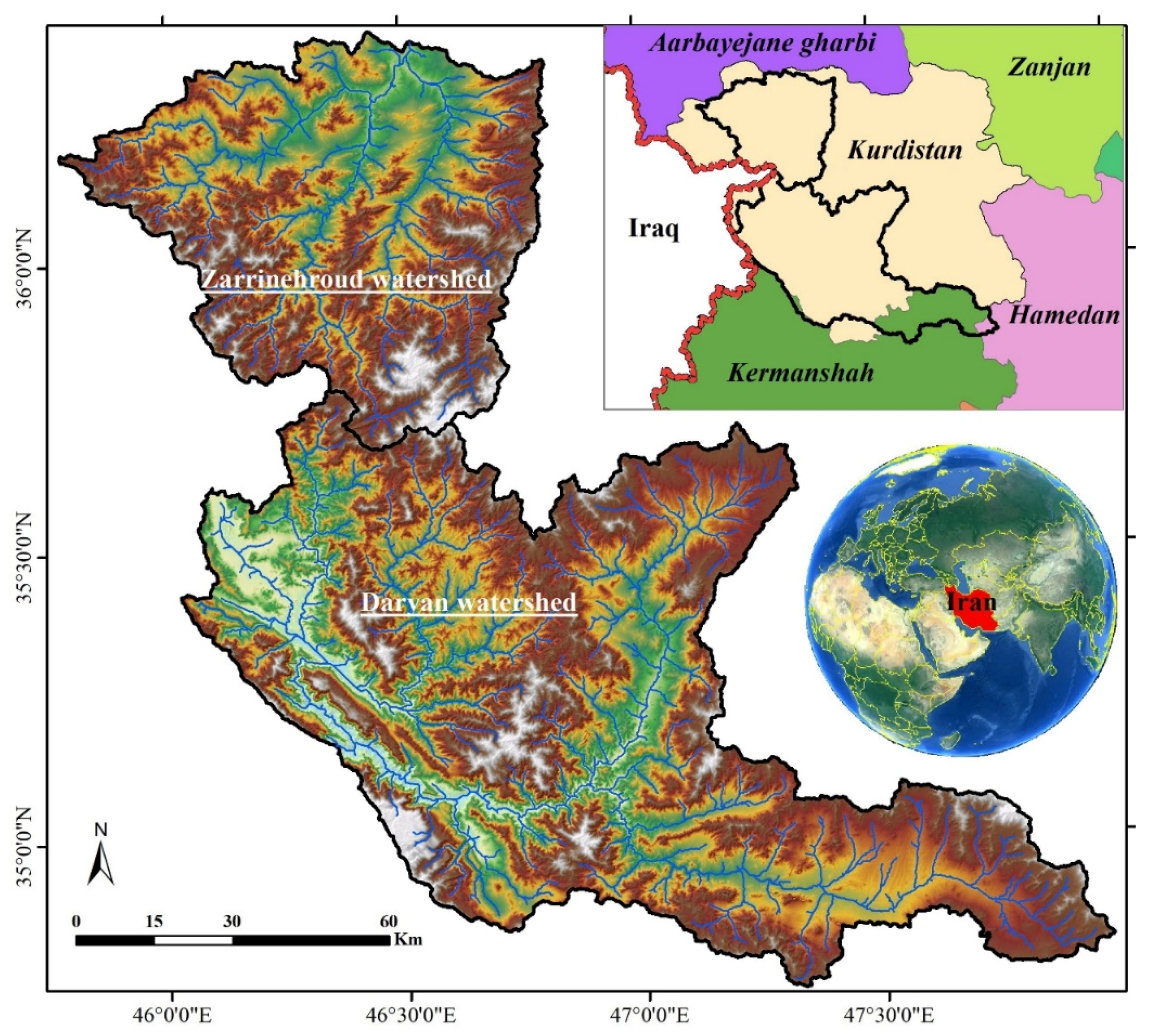
2.1. Study Area

This research was conducted in two regions of Iran: the Zarrinehroud (4514 km2) and the Darvan (938 km2) watersheds. Both watersheds are in western Kurdistan Province (Figure 1). The Zarrinehroud Watershed is located between 35°40′ and 36°24′N and 46°44′ and 46°48′E. The Darvan Watershed is between 34°45′ and 35°47′N and 46°02′ and 48°04′E. These watersheds were selected because they are snowy in some months of the year, and because snow avalanches frequently occur (Table 1). Steep-sided valley profiles and physiographic characteristics make them highly susceptible to snow avalanche activity. About 70% of annual precipitation occurs between November and May, and is often snow. Rural settlements in both study areas are often exposed to snow avalanches. Heavy snowfall and avalanches block rural and urban road networks during some parts of the year. Snow avalanches killed four people and injured 28 more in 2015–2018.

2.2. Dataset Used

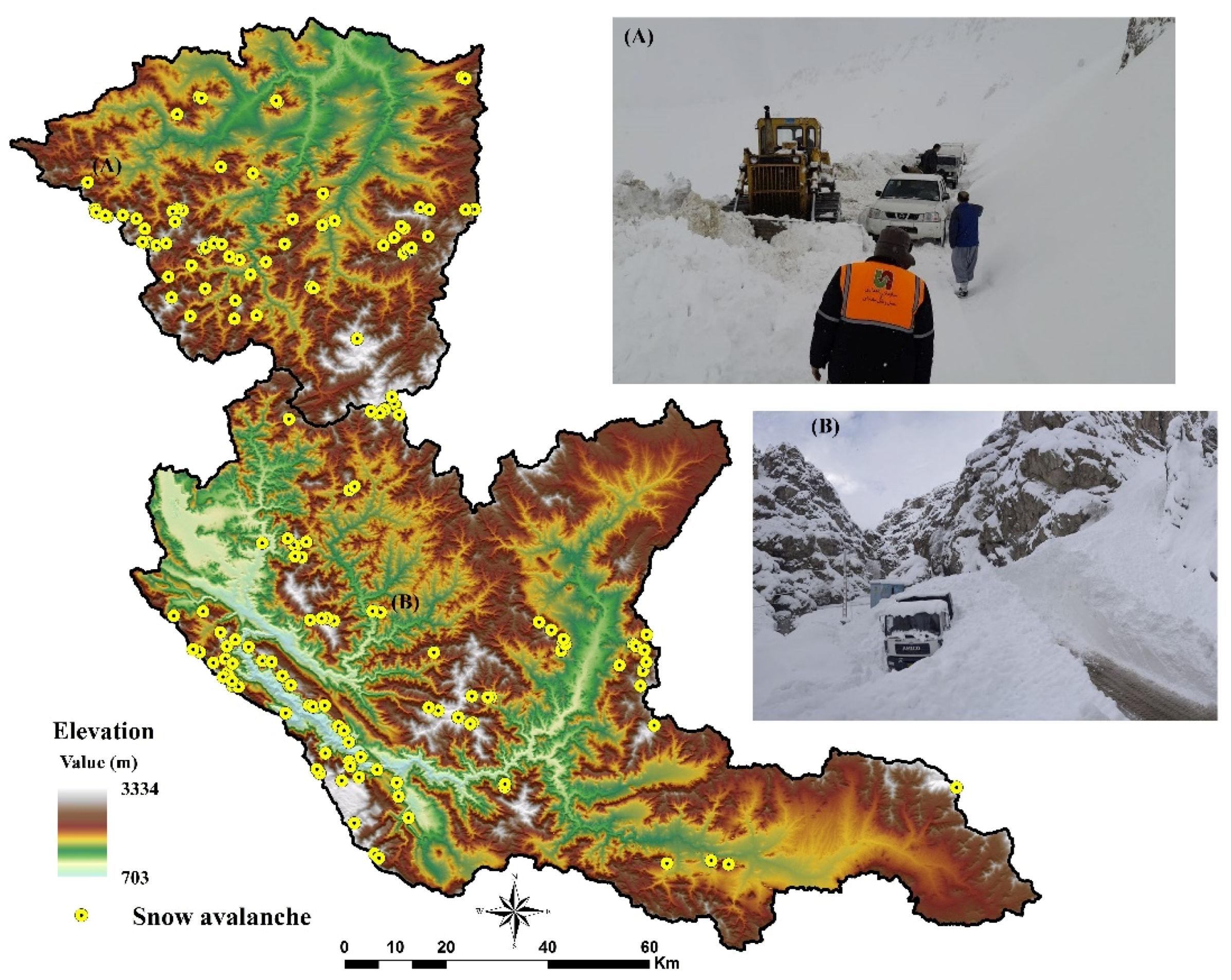
2.2.1. Snow Avalanche Inventory

Collecting and documenting previous snow avalanches is important for modeling the snow avalanche hazard [49,50]. Avalanche occurrence is the dependent variable in the modeling process. A database of snow avalanche occurrences was prepared through field observations and surveys in the winters of 2016, 2017 and 2018 (Figure 2).
These snow avalanches were mapped with a global positioning system (GPS) and Google Earth imagery. Only one point was mapped per snow avalanche to provide equal treatment of large and small snow avalanche occurrences, to reduce the effect of spatial autocorrelation between observations (especially when some points are considered for a snow avalanche), to avoid uncertainties in mapping snow avalanche boundaries. Some reports from the Road Organization added some avalanche locations to the database. A total of 72 and 105 snow avalanche locations were identified in the Zarrinehroud and Darvan watersheds, respectively.

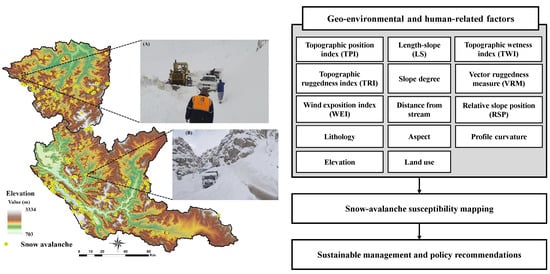
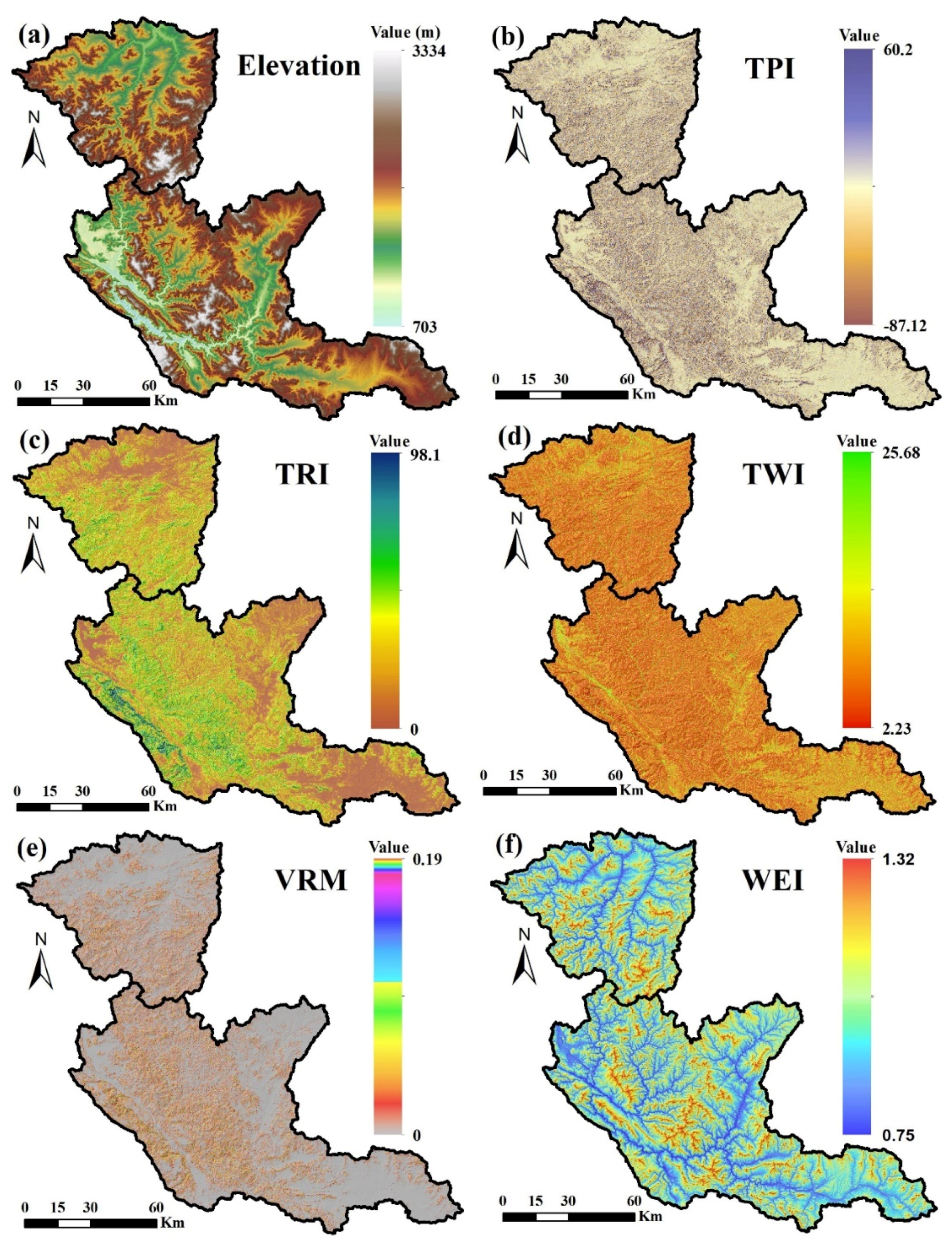
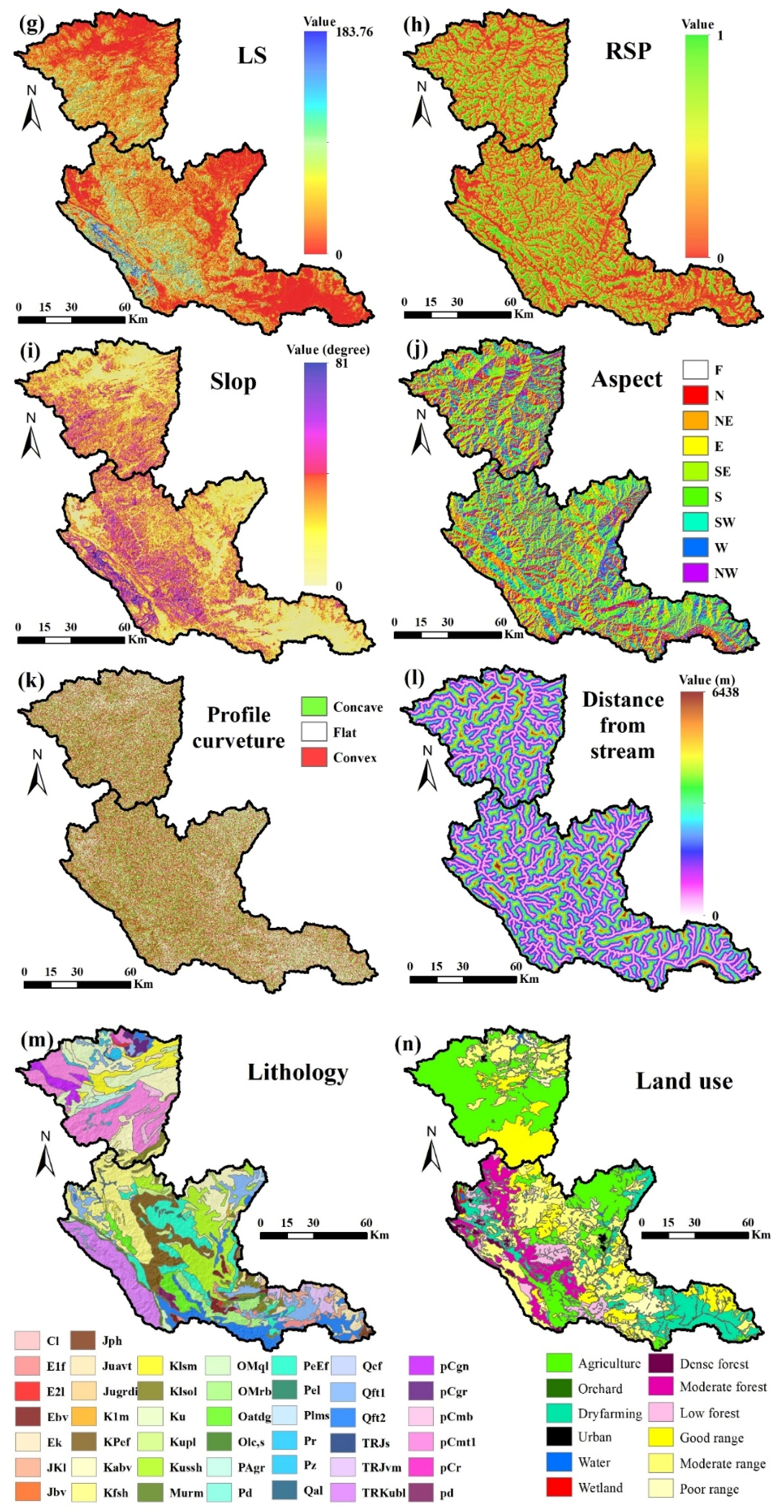
2.2.2. Factors Influencing Snow Avalanches
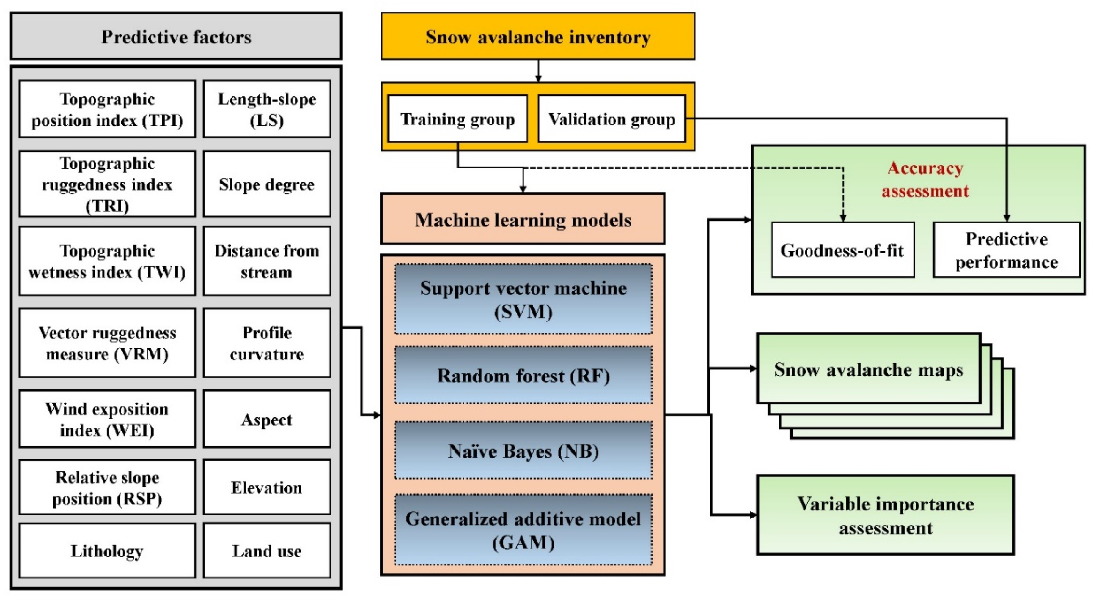
Geomorphological, topographical and environmental factors influence the snow avalanche occurrence. In spatial modeling, these factors are independent variables (hereafter termed predictive factors). There are no universal guidelines to select the main predictive factors.
Therefore, we selected them by reviewing the scholarly literature [1,12,13,50,51,52,53,54] and considering data availability. Kumar [49] stated that though meteorological conditions vary from year to year, the terrain and its characteristics are constant. Over an extended timeframe, these factors are suitable for snow avalanche susceptibility mapping. In this study, the predictive factors are elevation, topographic position index (TPI), topographic ruggedness index (TRI), topographic wetness index (TWI), vector ruggedness measure (VRM), wind exposition index (WEI), length-slope (LS), relative slope position (RSP), slope degree, aspect, profile curvature and distance from the stream (Figure 3).
(1) Elevation
Some measures of weather conditions such as temperature and wind speed vary with elevation. Therefore, elevation indirectly affects the initiation of snow avalanches [12,50]. An elevation map with a resolution of 20 m was obtained from the Iranian Department of Water Resources Management (IDWRM). Elevations range from 703 to 3328 m in the Darvan Watershed, and from 1372 to 3141 m in the Zarrinehroud Watershed (Figure 3a).
(2) TPI
The TPI reflects the corresponding position of each pixel in the landscape. In fact, TPI measures the difference between the elevation at the central point of the pixel, and the mean elevation of a predetermined neighborhood of pixels as the relative topographic position. This variable has been applied in the fields of hydrology [55], geomorphology [56], climatology [57], risk management [58] and snow avalanche risk assessment [50]. In addition, it is useful for landform classification and can be computed with De Reu [59] (Equation (1)):
T P I = E p i x e l E s u r r o u n d i n g
where Epixel and Esurrounding are the elevation of the cell and the mean elevation of the neighboring pixels, respectively. TPI maps were produced for both study areas in SAGA-GIS [60]. TPI ranges from −97 to 95.1 m in the Darvan Watershed, and from −78.8 to 69.6 m in the Zarrinehroud Watershed (Figure 3b).
(3) TRI
TRI is increasingly being used in a topographical analysis to characterize the convex or concave forms of slopes [60,61]. It was developed by Riley [62] and can be computed with (Equation (2)):
T R I = | x | ( m a x 2 m i n 2 )
where x shows the elevation of each neighbor cell (0,0). In addition, min and max depict the smallest and largest elevation value among neighboring pixels, respectively. TRI also was calculated and mapped in SAGA-GIS [26]. TRI values in the Darvan Watershed range from 0 to 98.1 m, and the range is <82.3 m in the Zarrinehroud Watershed (Figure 3c).
(4) TWI
TWI characterizes the influence of topography on hydrological processes and is used to infer the spatial distributions of wetness conditions [63] and snow avalanche activity [50]. It can be calculated with (Equation (3)) [64]:
T W I = l n ( α t a n β )
where α denotes upslope area which drains to a point, and β is the slope angle at the pixel. TWI has a range between 1.9 and 25 in the Darvan Watershed and from 2 to 24.9 in the Zarrinehroud Watershed (Figure 3d).
(5) VRM
VRM is a geomorphometric factor often used in geomorphological studies [65]. VRM measures the ruggedness of the landscape and provides vital information for snow avalanche prediction [50]. As explained by Kumar et al. [64,65,66], terrain roughness prevents the formation of a uniformly weak layer of snow and can block the downward movement of the snowpack. On the other hand, terrain roughness may destabilize this snowpack by increasing the stress on it [66]. VRM ranges from 0 to 0.206 in the Darvan Watershed, from 0 to 0.2 in the Zarrinehroud Watershed (Figure 3e).
(6) WEI
Wind not only causes drifting and redistribution of snow (i.e., snow-depth distribution), but also influences energy exchange, and can strongly influence the melting and freezing of snow and ice [67]. The wind is believed to be one of the main snow avalanche predictive factors, since when its velocity is reduced leeward of the ridges, additional snowfall accumulates there [68,69]. The wind exposition index (WEI) was calculated and mapped in SAGA-GIS [26]. WEI calculates the average wind effect from all directions using an angular step [70] (Figure 3f).
(7) LS
LS is a compound geomorphometric factor that has been used in geomorphological and environmental hazard studies [71,72,73]. LS was computed using one of the modules available in SAGA-GIS [26]. In the Darvan Watershed, LS ranged from 0 to 183.7. While the range LS was from 0 to 54.3 in the Zarrinehroud Watershed (Figure 3g).
(8) RSP
RSP measures topographic exposure and is bounded by 0 and 1, which represent valley bottom and ridge top, respectively [74,75]. The position of each pixel in a terrain reflects its relative hydrological and geomorphological processes which consequently influence stability [76]. RSP varies from 0 to 1 in both watersheds (Figure 3h).
(9) Slope
The slope is one of the most important terrain factors for mapping the snow avalanche susceptibility [12]. It mediates the vector of the acceleration due to gravity with surface support and friction, and can dictate the shear stress and shear strength that interacts to initiate avalanches. In this study, slope degree was calculated with a digital elevation model (DEM). The slope varies between 0° and 78.1° in the Darvan Watershed and from 0° to 76.3° in the Zarrinehroud Watershed (Figure 3i).
(10) Aspect
There is a significant correlation between aspect and snow avalanches [12,77]. Aspect strongly affects solar energy concentration, wind exposure, snowpack accumulation, snowmelt dynamics and vegetation. In both Darvan and Zarrinehroud watersheds, slopes facing northward are mostly shady, and snowpack is unstable for more extended periods annually. Southward facing slopes receive more insolation, and their snowpack is comparatively stable and resistant to snow avalanches [78]. The maps of aspect were generated from the DEM data (Figure 3j).
(11) Profile curvature
Profile curvature is vital in avalanche risk analysis because it directly influences shear stress and snowpack movement [49,79,80]. Plan curvature is classified as either concave, flat, or convex. Generally, concave surfaces are stable, while convex slopes promote instability in snow cover. The profile curvature maps were generated from the DEM (Figure 3k).
(12) Distance from stream
Distance from stream contributes to hydrological processes and various natural hazards [81,82]. This factor can be used to infer the spatial patterns of soil moisture and subsurface runoff dynamics, which affect the types of vegetation present in a landscape and their conditions. This factor was calculated using the Euclidian Distance tool in ArcGIS (Figure 3l).
(13) Lithology
Lithology dictates many surface features. In general, rocky outcrops increase surface roughness and decrease the downslope movement of the snowpack [1]. Lithology maps of the watersheds at a scale of 1:100,000 were extracted from a digitized geology map of Kurdistan Province (Figure 3m).
(14) Land use
Land use is one of the most critical factors in snow avalanche assessment [83]. For example, dense forest can prevent the initiation of snow avalanches. A 1:50,000 land-use map was acquired from the Iranian Department of Water Resources Management (IDWRM). Its data were verified with ground-truthing field investigations. The predominant land uses in the two watersheds are dissimilar. For example, while the dominant land cover in the Darvan Watershed is forested land, there is no forested land in the Zarrinehroud Watershed (Figure 3n).

2.3. Methodology

The steps (Figure 4) to complete analysis of the conditions promoting avalanches are: (1) map the 14 potential predictive factors, (2) develop four machine-learning models for avalanche prediction, (3) evaluate the accuracy of the models using statistical criteria, and (4) determine the relative importance of all factors for predicting the location of snow avalanche development.

2.3.1. Generating Snow Avalanche Hazard Maps

Four advanced ML models—SVM, RF, NB and GAM—were employed to predict snow avalanches.
(1) Support vector machine (SVM)
The SVM, which is known as the maximum-margin method, is used for modeling and spatial prediction of snow avalanche potential. SVM is based on statistical learning theory that can find an optimal clustering hyperplane among the input data by transforming the input space into a higher-dimensional feature space [84,85]. This transformation employs non-linear transformers to specify the best separating hyperplane. The best hyperplane is found when the Euclidean distance of the separating margins between the defined classes of the problem is at a maximum [86]. Kernel functions have been developed and used for solving non-linear life phenomena [87]. The most popular kernel functions are given in Table 2. The variables d, σ and b are kernel parameters for each kernel function, and these parameters, along with the penalize parameter (C), affect the efficiency of SVM. The selection of kernel function is an important step for the generalizability of SVM. The RBF is the most commonly used kernel function, especially for the non-linear problems like natural-hazard probability modeling. In this study, the RBF was therefore selected. Increasing the C parameter leads to an over-fitted model, while the σ parameter controls the shape of the clustering hyperplane, and consequently, the overall classification accuracy [88]. An optimization technique based on the genetic algorithm was used to determine the most optimal values of the RBF kernel. The optimal values of C and σ were 165 and 0.6, respectively.
(2) Random forest (RF)
The RF model is an ensemble classifier, which combines multiple decision trees to classify the input dataset [89,90]. Training-set overfitting of decision trees’ habit was corrected by RF; alternatively, it can be described as a set of decision trees that take a dataset and iteratively re-sample it based on the training data [91]. In this method, n tree bootstrap samples are created from the original dataset. Then, an unpruned classification or a regression tree is established for each of the bootstrap samples. The outcome is the average of the results of all of the n trees. A random set of features is selected each time to predict output, and each output is weighted by the value derived from the votes that it receives [30]. The majority voting based on the outputs of estimated decision trees converges to a single decision tree for the final classification [92]. Using the single decision tree overcomes the uncertainty problem and results in higher prediction accuracy [93,94]. Deriving the high variance from different decision trees is crucial for classification by RF. The literature reports that RF classifications yield good results when used to classify satellite imagery. Hence, RF is one of the most operative, non-parametric, ensemble learning approaches in susceptibility modeling and mapping. We repeated the re-sampling process ten times to get the best result. A set of observations that are not used for tree growth are termed the ‘out-of-bag (OOB)’ sample. The OOB sample is used to estimate the prediction error and then to determine variable importance. Each tree provides a prediction for its out-of-bag sample, and the average of these results for all trees performs an in situ cross-validation that is known as the ‘out-of-bag validation’ [91]. In addition, there are three training parameters for RF modeling: ntree (the number of trees in the forest), mtry (the number of predictors at each split) and nodesize (the minimal size of the terminal nodes of the trees). When ntree becomes small, the results deteriorate considerably. If ntree is increased above the optimum value, it causes a general increase in computational cost, though the results will not be improved notably. When mtry is very small, not enough predictor variables are entered at each split, and consequently, the predictive capability of each tree decreases [89]. The default value of ntree is 500 trees, whereas one third of total number of the variables. The default value of nodesize is one. In this study, the ntree values were tested from 500 to 5000 with 100 intervals, and mtry was tested from 1 to 14 using a single interval. The optimization was done using the calibration dataset and the root mean square error (RMSE). A ntree of 4200 and a mtry of 6 resulted in the highest accuracy for snow avalanche modeling.
(3) Naïve Bayes (NB)
The naïve Bayes (NB) ML model is a widely used classifier, primarily in data mining studies. The popularity of this model is due to the simplicity of its construction and runtime [95,96]. Furthermore, the NB model is robust and is less affected by noise and irrelevant attributes [97]. The NB classifier is a probabilistic model based on the Bayesian probability and Bayes’ theorem [98]. In this model, there is an assumption that all the attributes are fully independent, which is called the conditional independence assumption [99].
This model is used to determine and select the classes that maximize the posterior probabilities using the following steps: (a) Collecting the samples, (b) assessing a prior probability for any defined class, (c) assessing the mean value of defined classes, (d) creating the covariance matrix and assessing the inverse and determinant for any defined class [100] and (e) structuring the discriminant function for any defined class [101]. There exist different kernel functions such as linear, polynomial and Gaussian [102]. In this study, the polynomial kernel was used and it was defined previously in Table 2.
(4) Generalized additive model (GAM)
The generalized additive model (GAM), another ML technique introduced by Hastie and Tibshirani [54], was also used to predict the likely locations of snow avalanches. The GAM is a semi-parametric extension version of the generalized linear model that can combine both linear and nonlinear relationships between the input predictors and the inventory dataset to determine the target data and the responses. Nonlinear problems apply smooth functions of covariance to transform the predictors [103]. The summation of smoothers in the predictors is considered the response [104]. Therefore, the GAM generates a flexible classification of the dependence of the response on the covariates, which makes it practical for analysis of nonlinear responses to changing site conditions. It is, consequently, useful for spatial problems like natural hazard susceptibility modeling and mapping [96]. In the GAM model, the additive predictor η(X) is used as an alternative to the common linear predictor in the GLM. The simple form of the GAM is described by Equation (4):
g ( E ( Y i ) ) = β 0 +   f 1 ( X 1 ) + + f m ( X m )
where the expectation of the variable Y is defined by E(Y); the function of g(.) is considered as the link function; β 0 is the intercept; and f i ( X i ) is the smoothing function of the input factor variable of X i [105]. This model follows the three steps: (a) Determination of the distribution of the response variable and its corresponding link function, (b) determination of the parameters as smoothing functions and the basis dimension “k”, and (c) model optimization using contour plots.

2.3.2. Accuracy Assessments

The performances of the snow avalanche hazard models were evaluated with a k-fold spatial cross-validation approach, as described by Goetz et al. [50,51]. The inventory dataset is randomly partitioned into k disjoint sets, and one subset at a time is used for model validation while the combined remaining k-1 subsets are utilized for model calibration/training. The R package “sperrorest” developed by Brenning [106] was used for designing a ten-fold cross-validation method.
In this study, two standard evaluation metrics, the area under the receiver operating characteristics curve (AUROC) and true skill statistics (TSS), were used. AUROC is a cutoff-independent metric, whereas TSS is a cutoff-dependent metric.
(1) The AUROC metric
The accuracy assessment evaluated the effectiveness of each ML model by analyzing the uncertainty among the resulting susceptibility maps as compared to the inventory data set. The (AUROC) curve technique was selected for this comparison. It is commonly used to characterize the quality of the resulting susceptibility-prediction maps, particularly in the geosciences [107,108]. The plotted curves display the trade-offs between the false positive rate (FPR) and the true positive rate (TPR), on the X and Y axis, respectively. AUROC is an accuracy index. Values closer to one indicate that the output map provides higher quality predictions [109,110]. AUROC curves were calculated for all resulting snow avalanche susceptibility maps. To assess goodness-of-fit, the training pixels were used. Predictive performance of the models, however, was assessed with the validation pixels.
(2) TSS metric
The true skill statistics is the other accuracy assessment technique used. It was first proposed by Allouche et al. [111], and is based on the components of a confusion matrix which is generated from the number of matches and mismatches between the inventory data and the modeled results [111].
The TSS can be calculated with Equation (5):
T S S   = T P R + T N R 1
where TPR and TNR are defined by Equations (6) and (7):
T P R = TP TP + FN
T N R = TN TN + FP
where TN (true negative) and TP (true positive) are the number of pixels that are correctly classified whereas FN (false negative) and FP (false positive) are the numbers of pixels erroneously classified. Another performance metric is Matthews correlation coefficient (MCC) that can be calculated as follows (Equation (8)):
M C C = ( T P × T N ) ( F P × F N ) ( T P + F P ) ( T P + F N ) ( T N + F P ) ( T N + F N )
The values of the TSS range from −1 to 1; the closer the value is to 1, the better the performance [112]. Both AUROC and TSS evaluation metrics were calculated using a GIS-based extension—performance measure tool (PMT)—which were developed by Rahmati et al. [92]. Besides, these evaluation metrics were calculated in terms of both goodness-of-fit (accuracy of the model in the training step) and predictive performance (accuracy of the model in the validation step).

2.3.3. Ensemble Modeling

In general, all the ensemble techniques use the weighted integration of individual models to come up with the outcome. However, the way of calculating these weights are different. In this study, an ensemble method which has proposed by Pourghasemi et al. [113] was used. The ensemble map can be generated using Equation (9):
E M = i = 1 n ( A U R O C i × M i ) i = 1 n A U R O C
where EM is the resulted ensemble model, AUROCi is the AUROC value of the ith single model (Mi).

2.3.4. Statistical Comparison of Models

Friedman Test

The Friedman test is a non-parametric test that has been known as one of the most reliable tests for multiple comparisons to discover significant differences among models [114]. As one of the most important characteristics, it does not assume normal distributions or homogeneity of variance for the compared random variables. The null hypothesis (H0) assumes no difference between the performances of the snow avalanche models. In other words, the null hypothesis of the Friedman test is that all models are equivalent based on their average ranks. If the p-value is less than the significance level (α = 0.05), and the chi square value (χ2) is higher than the standard value (3.841), the null hypothesis is rejected. Since this test does not provide pairwise comparison of these models, it only provides statistical differences for all the models.

Wilcoxon Signed-rank Test

In order to statistically compare the differences of models, the Wilcoxon signed-rank test, a nonparametric method, was performed. This method is used to test the hypothesis that the means of the first sample is equal to the means of the second sample. This test evaluates the significance of differences between some models based on two statistical components including z and p. When the z value exceeds the critical range (from −1.96 to +1.96) and also the p value is less than the significant level (α = 0.05), then the null hypothesis is rejected (i.e., these models are statistically different). Similar to the Friedman test, the Wilcoxon signed-rank test does not assume normal distributions or homogeneity of variance for the compared random variables.
This relaxed assumption ensures the generality of the test. As discussed by Lin et al. [115], it is appropriate that we conduct the Wilcoxon signed-rank test instead of the paired t-test when comparing two models.

3. Results

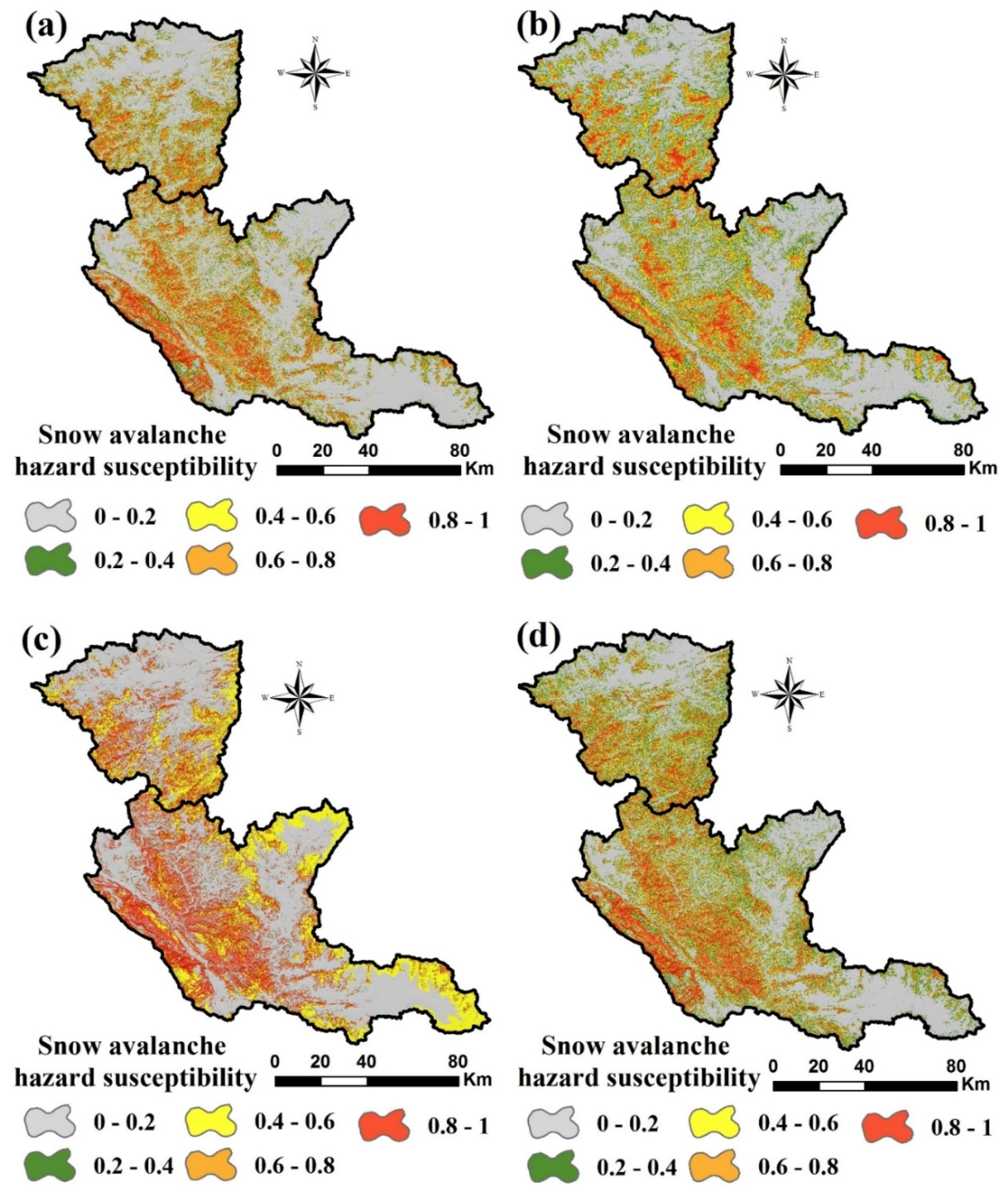
3.1. Snow Avalanche Hazard Maps

The avalanche hazard maps predicted by the four models generally exhibit the same spatial patterns, although the details of each model differ (Figure 5). In the Zarrinehroud Watershed, areas near the ridgeline (i.e., the drainage divide of the watershed), especially in the southern parts of the watershed, are identified as most susceptible to snow avalanches. In the Darvan Watershed, a strip along the southwestern border of the watershed, extending to the center of the watershed, is the corridor of highest risk. Low-susceptibility zones in both watersheds are, unsurprisingly, in the lowlands.
Predicted snow avalanche pixels in all four maps of the study area were categorized into five susceptibility classes based on their susceptibility values: very low (0–0.2), low (0.2–0.4), medium (0.4–0.6), high (0.6–0.8) and very high (0.8–1.0) (Figure 5). The areas contained in the very high class vary between 7% and 16%, where the average is 11.5% for the models (Table 2). The high-susceptibility zones are approximately 10.5% of the basin. In total, about one-fifth of the study area could be regarded as avalanche-prone. In both basins, more than 60% of the study areas were categorized as low and very low susceptibility.
After preparing the snow avalanche hazard map by the ensemble model, it was reclassified to five classes: very low (0–0.2), low (0.2–0.4), medium (0.4–0.6), high (0.6–0.8) and very high (0.8–1) (Figure 6). Unsurprisingly, both individual and ensemble models show the same overall spatial pattern with some differences. The relative area of each class was shown in Table 3.

3.2. Performance of Models

Considering the goodness-of-fit, AUROC values of 0.981 (RF), 0.977 (ensemble), 0.972 (SVM), 0.932 (NB) and 0.924 (GAM) were observed for the Darvan Watershed predictions (Table 4, Figure S1). In the Zarrinehroud Watershed, the values of 0.973 (RF), 0.968 (ensemble), 0.965 (SVM), 0.941 (NB) and 0.934 (GAM) were obtained. In terms of TSS and MCC, the RF model generated the most accurate predictions in both the Darvan Watershed (TSS = 0.893, MCC = 0.884) and the Zarrinehroud Watershed (TSS = 0.882, MCC = 0.866).
The next best is ensemble (TSS = 0.886 and MCC = 0.871 in Darvan and TSS = 0.877 and MCC = 0.862 in Zarrinehroud), SVM (TSS = 0.882 and MCC = 0.863 in Darvan, and TSS = 0.863 and MCC = 0.859 in Zarrinehroud), and then NB (TSS = 0.791 and MCC = 0.855 in Darvan, and TSS = 0.835 and MCC = 0.825 in Zarrinehroud). The GAM (TSS = 0.75 and MCC = 0.812 in Darvan, and TSS = 0.83 and MCC = 0.808 in Zarrinehroud) is the least accurate model. Goodness-of-fit indicates only how well the model fit the training dataset. The predictive capacities and generalizability of the models cannot be evaluated based on the goodness-of-fit, as it uses the data with which the models were built [43]. Therefore, the accuracy of the models is best assessed with the validation data.
Analysis of the validation step reveals that the ensemble model (AUROC = 0.966 in Darvan and AUROC = 0.958 in Zarrinehroud) was a slightly better predictive performance than RF (AUROC = 0.964 in Darvan and AUROC = 0.956 in Zarrinehroud) for both the watersheds (Table 4, Figure S2). The TSS and MCC metrics also indicate that the ensemble model achieved the best predictive performance in both the Darvan (TSS = 0.865, MCC = 0.861) and Zarrinehroud (TSS = 0.877, MCC = 0.841) watersheds, followed by RF model (TSS = 0.862, MCC = 0.865 in Darvan and TSS = 0.881, MCC = 0.854 in Zarrinehroud). After the ensemble and RF, SVM was the third best model, producing better predictions in both the Darvan (AUROC = 0.955, TSS = 0.844, MCC = 0.858) and Zarrinehroud (AUROC = 0.948, TSS = 0.875, MCC = 0.832) watersheds. SVM followed by NB that had an AUCROC of 0.914, a TSS of 0.727, and MCC of 0.847 in the Darvan Watershed and AUROC = 0.922, TSS = 0.853, and MCC = 0.804 for Zarrinehroud). GAM’s values were AUROC = 0.896, TSS = 0.714, and MCC = 0.796 for Darvan and AUROC = 0.905, TSS = 0.816, and MCC = 0.793 for Zarrinehroud. Although the accuracies of SVM, NB and GAM were slightly lower than the ensemble and RF models in both study areas, all four models rate “very good” (0.8 < AUROC < 0.9) or “excellent” (AUROC > 0.9) in their avalanche-predicting performance [116,117].

3.3. Statistical Comparison of Models

3.3.1. Friedman Test

The results of the Friedman test in the Zarrinehroud and Darvan watersheds (Table 5) showed that both the p-value and chi square value (χ2) of four models are far from the standard values of 3.841 and 0.05, respectively. Therefore, the null hypothesis is rejected. This clearly indicates that the differences among the models are statistically significant. However, since the results of the Friedman test highlights only the significant differences of performance of all the employed models, the result is not able to provide comparisons between these two models.

3.3.2. Wilcoxon Signed-Rank Test

Results of the Wilcoxon signed-rank test in both Darvan and Zarrinehroud watersheds were summarized in Table 6. In the Darvan Watershed, not only the p values were far from the standard value of 0.05, but also these z values were out of the standard range (from −1.96 to +1.96). These conditions were observed for both the Zarrinehroud and Darvan watersheds. Therefore, the differences of all four models are statistically significant.

3.4. Variable Importance

The degree to which each contributing factor helps to discern locations of snow avalanche risk was determined with the RF model (Table 7). A higher mean square error (MSE) value, determined by removing a variable from the modeling, indicates that it is of greater importance. The results demonstrate that LS, lithology and RSP are the three main conditioning factors that promote avalanche likelihood with 63.2%, 54.6% and 41.3% in Darvan Watershed and 62.8%, 55.2% and 39.8% for Zarrinehroud Watershed. TRI (36.5% in Darvan, 37.5% in Zarrinehroud), slope (32.4% in Darvan, 33.4% in Zarrinehroud), TPI (28.2% in Darvan, 29.5% in Zarrinehroud), profile curvature (22.1% in Darvan, 24.4% in Zarrinehroud), elevation (19.8% in Darvan, 21.7% in Zarrinehroud), VRM (17.5% in Darvan, 16.5% in Zarrinehroud), land use (14.7% in Darvan, 14.2% in Zarrinehroud) and aspect (13.2% in Darvan, 12.9% in Zarrinehroud) had more moderate contributions to the models. Distance from a stream and TWI were the least important factor in both watersheds (i.e., less than ten percent).

4. Discussion

4.1. The Performance of Models

Since the performances of RF, NB and GAM in the field of snow avalanche hazard have not been evaluated previously, it is impossible to directly compare these results to previous studies. The accuracy of SVM, however, confirms results achieved by Choubin et al. [24]. Numerous studies have applied AHP models which are based on the knowledge and judgments of experts, but the reliance on subjective expert input can be the primary drawback of using them [118]. In the case of avalanche modeling with AHP, the weighting of avalanche-promoting factors used in the models can be very inefficient. Results of this study showed that the ensemble model outperformed individual models in both watersheds. Among individual models, RF had the highest predictive performance and was slightly weaker than the ensemble model. In this study, SVM was used as a benchmark for comparing its results with other individual and ensemble models. Our results also confirmed the study of Choubin et al. [24], who suggested SVM for snow avalanche hazard mapping.
The outstanding performance of RF is due to its key advantages: capability to determine variable importance, non-parametric relationships, robustness to outliers and noise, high classification accuracy and internal, unbiased determination of the generalization error through the out-of-bag (OOB) factor. Rahmati et al. [92] have confirmed the capacities of ML models for analyzing complicated relationships of geoenvironmental, topohydrological and extreme natural processes or events. The two reasons for the better performance of ML models over bivariate and multivariate models is that no statistical assumptions are made, and they can handle data from various measurement methods [26,119,120].

4.2. Statistical Comparison of Models

In addition to the evaluation of the performance of the models, the exploration of their statistical differences is necessary [121]. As discussed by Bui et al. [16], these differences originated from the variability of model structures and their spatial prediction patterns. This issue has not yet been investigated for snow avalanche modeling; hence, it is not easy to compare our achievements with previous studies. This motivated us to select two case studies with the same predictive factors and models to fairly judge the statistical differences between the models. This issue was addressed in this study with the evaluation and comparison of different ensemble and standalone machine learning models. All standalone and ensemble models were statistically different for both Darvan and Zarrinehroud watersheds.

4.3. Variable Importance

It is logical to say that not all the selected conditioning factors (independent variables) are strong predictors, and in some cases, some of them generate noise and reduce the accuracy of predictions. Therefore, feature selection should be investigated [122]. Generally speaking, users and decision makers feel more comfortable in the practical application of a model if they have a clear understanding of the predictive factors that favorably contribute to the modeling process. Previous researchers have used a wide array of geomorphometric and topohydrological factors to spatially model snow avalanches. Our findings are broadly consistent with Choubin et al. [24]. They found that the TPI strongly influenced the spatial distribution of snow avalanches. This is also in line with the results of Kumar [64,65], who used the AHP method to map the snow avalanche hazard; their study indicated that slope was the most consequential terrain parameter, and ground cover was the least important. Previous studies, however, have not considered a more comprehensive set of geomorphometric factors, such as LS and RSP, so more profound comparisons are not possible. The results of variable importance highlighted that even factors such as distance from the stream and TWI that had less contributions to the modeling process can improve the accuracy of the model.

5. Conclusions

This study used an innovative method to scrutinize the capability, and efficiency of four ML approaches—RF, SVM, NB and GAM—to spatially model snow avalanches. To determine how robust and generalizable they are, this study was undertaken in two watersheds (the Darvan and the Zarrinehroud) in Kurdistan Province, Iran. A wide array of geomorphometric, topo-hydrologic and geo-environmental factors were employed in combination with a snow avalanche inventory to develop the models. The following conclusions can be drawn:
(1) The results demonstrate that the ensemble model slightly outperformed all individual models in terms of the predictive performance in both Darvan (AUROC = 0.966, TSS = 0.865, MCC = 0.861) and Zarrinehroud (AUROC = 0.958, TSS = 0.877, MCC = 0.841) watersheds. Among individual models (i.e., RF, SVM, NB and GAM), the RF was the best model for predicting locations susceptible to snow avalanches in both the Darvan (AUROC = 0.964, TSS = 0.862, MCC = 0.865) and the Zarrinehroud (AUROC = 0.956, TSS = 0.881, MCC = 0.854) watersheds. This can be determined with both cutoff-dependent and cutoff–independent evaluation metrics. Importantly, the model performance of RF was relatively similar to the ensemble model, and always achieved a top two estimation in both goodness-of-fit and predictive performance, usually just behind the ensemble model. SVM and NB also performed at excellent levels (AUROC > 0.9). GAM produced a very good result (0.8 < AUROC < 0.9) for both watersheds. Since all four machine learning models achieved very good or excellent results, these models can be regarded as effective choices for spatially modeling the snow avalanche hazard. Furthermore, the statistical analysis clearly indicates that the results of the models are significantly different.
(2) The snow avalanche hazard maps for the Darvan and Zarrinehroud watersheds indicate the regions that are most likely to see snow avalanches, and they also provide useful information to undergird snow avalanche risk assessments, land use planning and infrastructure development decision making. The ensemble map indicates that approximately 26% of the Darvan Watershed and 21% of the Zarrinehroud Watershed is classified as having high or very high avalanche risk. Some areas along the main roads through the watersheds fall into these areas, and need to be carefully evaluated for safety.
(3) The variable-importance assessment also highlights that LS, lithology and RSP are the most significant factors for predicting a snow avalanche hazard. Avalanche prediction is a complex procedure; therefore, the results of this study can improve our understanding of the snow avalanche hazard. It is highly recommended that this information be employed by decision-makers and used in future studies. Managers should take these findings into account and apply this information for the management of avalanche hazards in the high- and very-high-risk zones.
(4) Although the efficiency and applicability of four advanced machine learning models have been evaluated, there are still other modeling approaches that should be used for snow avalanche hazard mapping. Therefore, further studies focusing on the capability of other machine learning models (e.g., XGBoost, logistic model tree, etc.) in this field of study is suggested.

Supplementary Materials

The following are available online at https://www.mdpi.com/2072-4292/11/24/2995/s1, Figure S1: ROC curves in goodness-of-fit: (a) RF in Darvan, (b) RF in Zarinehroud, (c) SVM in Darvan, (d) SVM in Zarinehroud, (e) NB in Darvan, (f) NB in Zarinehroud, (g) GAM in Darvan, (h) GAM in Zarinehroud, (i) the ensemble model in Darvan, and (j) the ensemble model in Zarinehroud; Figure S2: ROC curves in predictive performance: (a) RF in Darvan, (b) RF in Zarinehroud, (c) SVM in Darvan, (d) SVM in Zarinehroud, (e) NB in Darvan, (f) NB in Zarinehroud, (g) GAM in Darvan, (h) GAM in Zarinehroud, (i) the ensemble model in Darvan, and (j) the ensemble model in Zarinehroud.

Author Contributions

Conceptualization, O.R. and O.G.; methodology, O.R., O.G., T.T., F.M., F.F., S.P., and D.T.B.; validation, J.P.T., S.P. and P.-T.T.N.; formal analysis, O.R.; investigation, T.T.; writing—original draft preparation, O.R., O.G., T.T., and S.P.; writing—review and editing, O.R., J.P.T., P.-T.T.N., and D.T.B.

Funding

This research was support by the GIS research group, Ton Duc Thang university, Ho Chi Minh city, Vietnam. The open access was supported by University of South-Eastern Norway, Bø i Telemark, Norway

Acknowledgments

We thank the Iranian Department of Water Resources Management (IDWRM), Iranian Department of Geology, the Road Organization of Iran, and Natural Resource Department and Regional Water Company (NRDRWC) for providing data and maps. We greatly appreciate the anonymous reviewers for their constructive comments that helped us to improve the paper.

Conflicts of Interest

The authors declare that they have no conflict of interest.

References

  1. Blahut, J.; Klimeš, J.; Balek, J.; Hájek, P.; Červená, L.; Lysák, J. Snow avalanche hazard of the Krkonoše National Park, Czech Republic. J. Maps 2017, 13, 86–90. [Google Scholar] [CrossRef] [Green Version]
  2. Abdollahi, S.; Pourghasemi, H.R.; Ghanbarian, G.A.; Safaeian, R. Prioritization of effective factors in the occurrence of land subsidence and its susceptibility mapping using an SVM model and their different kernel functions. Bull. Eng. Geol. Environ. 2018, 78, 4017–4034. [Google Scholar] [CrossRef]
  3. Arpaci, A.; Malowerschnig, B.; Sass, O.; Vacik, H. Using multi variate data mining techniques for estimating fire susceptibility of Tyrolean forests. Appl. Geogr. 2014, 53, 258–270. [Google Scholar] [CrossRef]
  4. Barbolini, M.; Natale, L.; Savi, F. Effects of release conditions uncertainty on avalanche hazard mapping. Nat. Hazards 2002, 25, 225–244. [Google Scholar] [CrossRef]
  5. Barbolini, M.; Pagliardi, M.; Ferro, F.; Corradeghini, P. Avalanche hazard mapping over large undocumented areas. Nat. Hazards 2011, 56, 451–464. [Google Scholar] [CrossRef]
  6. Bebi, P.; Kulakowski, D.; Rixen, C. Snow avalanche disturbances in forest ecosystems—State of research and implications for management. For. Ecol. Manag. 2009, 257, 1883–1892. [Google Scholar] [CrossRef]
  7. Bergua, S.B.; Piedrabuena, M.Á.P.; Alfonso, J.L.M. Snow avalanches, land use changes, and atmospheric warming in landscape dynamics of the Atlantic mid-mountains (Cantabrian Range, NW Spain). Appl. Geogr. 2019, 107, 38–50. [Google Scholar] [CrossRef]
  8. Bernhardt, M.; Zängl, G.; Liston, G.; Strasser, U.; Mauser, W. Using wind fields from a high-resolution atmospheric model for simulating snow dynamics in mountainous terrain. Hydrol. Process. Int. J. 2009, 23, 1064–1075. [Google Scholar] [CrossRef]
  9. Beven, K.J.; Kirkby, M.J. A physically based, variable contributing area model of basin hydrology/Un modèle à base physique de zone d’appel variable de l’hydrologie du bassin versant. Hydrol. Sci. J. 1979, 24, 43–69. [Google Scholar] [CrossRef] [Green Version]
  10. Bhargavi, P.; Jyothi, S. Applying naive bayes data mining technique for classification of agricultural land soils. Int. J. Comput. Sci. Netw. Secur. 2009, 9, 117–122. [Google Scholar]
  11. Böhner, J.; Antonić, O. Land-surface parameters specific to topo-climatology. Dev. Soil Sci. 2009, 33, 195–226. [Google Scholar]
  12. Breiman, L. Random forests. Mach. Learn. 2001, 45, 5–32. [Google Scholar] [CrossRef] [Green Version]
  13. Bühler, Y.; Kumar, S.; Veitinger, J.; Christen, M.; Stoffel, A.; Snehmani, S. Automated identification of potential snow avalanche release areas based on digital elevation models. Nat. Hazards Earth Syst. Sci. 2013, 13, 1321–1335. [Google Scholar] [CrossRef]
  14. Bühler, Y.; Rickenbach, D.; Stoffel, A.; Margreth, S.; Stoffel, L.; Christen, M. Automated snow avalanche release area delineation–validation of existing algorithms and proposition of a new object-based approach for large-scale hazard indication mapping. Nat. Hazards Earth Syst. Sci. 2018, 18, 3235–3251. [Google Scholar] [CrossRef] [Green Version]
  15. Bui, D.T.; Ngo, P.-T.T.; Pham, T.D.; Jaafari, A.; Minh, N.Q.; Hoa, P.V.; Samui, P. A novel hybrid approach based on a swarm intelligence optimized extreme learning machine for flash flood susceptibility mapping. Catena 2019, 179, 184–196. [Google Scholar] [CrossRef]
  16. Bui, D.T.; Tuan, T.A.; Klempe, H.; Pradhan, B.; Revhaug, I. Spatial prediction models for shallow landslide hazards: A comparative assessment of the efficacy of support vector machines, artificial neural networks, kernel logistic regression, and logistic model tree. Landslides 2016, 13, 361–378. [Google Scholar]
  17. Bunn, A.G.; Hughes, M.K.; Salzer, M.W. Topographically modified tree-ring chronologies as a potential means to improve paleoclimate inference. Clim. Chang. 2011, 105, 627–634. [Google Scholar] [CrossRef]
  18. Cama, M.; Lombardo, L.; Conoscenti, C.; Rotigliano, E. Improving transferability strategies for debris flow susceptibility assessment: Application to the Saponara and Itala catchments (Messina, Italy). Geomorphology 2017, 288, 52–65. [Google Scholar] [CrossRef]
  19. Casteller, A.; Häfelfinger, T.; Cortés Donoso, E.; Podvin, K.; Kulakowski, D.; Bebi, P. Assessing the interaction between mountain forests and snow avalanches at Nevados de Chillán, Chile and its implications for ecosystem-based disaster risk reduction. Nat. Hazards Earth Syst. Sci. 2018, 18, 1173–1186. [Google Scholar] [CrossRef] [Green Version]
  20. Che, V.B.; Kervyn, M.; Suh, C.E.; Fontijn, K.; Ernst, G.G.; Del Marmol, M.-A.; Trefois, P.; Jacobs, P. Landslide susceptibility assessment in Limbe (SW Cameroon): A field calibrated seed cell and information value method. Catena 2012, 92, 83–98. [Google Scholar] [CrossRef]
  21. Chen, W.; Pourghasemi, H.R.; Kornejady, A.; Zhang, N. Landslide spatial modeling: Introducing new ensembles of ANN, MaxEnt, and SVM machine learning techniques. Geoderma 2017, 305, 314–327. [Google Scholar] [CrossRef]
  22. Chen, W.; Pourghasemi, H.R.; Panahi, M.; Kornejady, A.; Wang, J.; Xie, X.; Cao, S. Spatial prediction of landslide susceptibility using an adaptive neuro-fuzzy inference system combined with frequency ratio, generalized additive model, and support vector machine techniques. Geomorphology 2017, 297, 69–85. [Google Scholar] [CrossRef]
  23. Chen, W.; Yan, X.; Zhao, Z.; Hong, H.; Bui, D.T.; Pradhan, B. Spatial prediction of landslide susceptibility using data mining-based kernel logistic regression, naive Bayes and RBFNetwork models for the Long County area (China). Bull. Eng. Geol. Environ. 2019, 78, 247–266. [Google Scholar] [CrossRef]
  24. Choubin, B.; Borji, M.; Mosavi, A.; Sajedi-Hosseini, F.; Singh, V.P.; Shamshirband, S. Snow avalanche hazard prediction using machine learning methods. J. Hydrol. 2019, 577, 123929. [Google Scholar] [CrossRef]
  25. Confortola, G.; Maggioni, M.; Freppaz, M.; Bocchiola, D. Modelling soil removal from snow avalanches: A case study in the North-Western Italian Alps. Cold Reg. Sci. Technol. 2012, 70, 43–52. [Google Scholar] [CrossRef]
  26. Conrad, O.; Bechtel, B.; Bock, M.; Dietrich, H.; Fischer, E.; Gerlitz, L.; Wehberg, J.; Wichmann, V.; Böhner, J. System for automated geoscientific analyses (SAGA) v. 2.1. 4. Geosci. Model Dev. 2015, 8, 1991–2007. [Google Scholar] [CrossRef] [Green Version]
  27. Covăsnianu, A. Mapping Snow Avalanche Risk Using GIS Technique and 3D Modeling: Case Study Ceahlau National Park. Available online: SSRN 1884082 2011 (accessed on 24 June 2019).
  28. Dadic, R.; Mott, R.; Lehning, M.; Burlando, P. Wind influence on snow depth distribution and accumulation over glaciers. J. Geophys. Res. Earth Surf. 2010, 115. [Google Scholar] [CrossRef] [Green Version]
  29. Darabi, H.; Choubin, B.; Rahmati, O.; Haghighi, A.T.; Pradhan, B.; Kløve, B. Urban flood risk mapping using the GARP and QUEST models: A comparative study of machine learning techniques. J. Hydrol. 2019, 569, 142–154. [Google Scholar] [CrossRef]
  30. de Bouchard d’Aubeterre, G.; Favillier, A.; Mainieri, R.; Saez, J.L.; Eckert, N.; Saulnier, M.; Peiry, J.-L.; Stoffel, M.; Corona, C. Tree-ring reconstruction of snow avalanche activity: Does avalanche path selection matter? Sci. Total Environ. 2019, 684, 496–508. [Google Scholar] [CrossRef]
  31. De Reu, J.; Bourgeois, J.; Bats, M.; Zwertvaegher, A.; Gelorini, V.; De Smedt, P.; Chu, W.; Antrop, M.; De Maeyer, P.; Finke, P. Application of the topographic position index to heterogeneous landscapes. Geomorphology 2013, 186, 39–49. [Google Scholar] [CrossRef]
  32. Duro, D.C.; Franklin, S.E.; Dubé, M.G. A comparison of pixel-based and object-based image analysis with selected machine learning algorithms for the classification of agricultural landscapes using SPOT-5 HRG imagery. Remote Sens. Environ. 2012, 118, 259–272. [Google Scholar] [CrossRef]
  33. Eckerstorfer, M.; Bühler, Y.; Frauenfelder, R.; Malnes, E. Remote sensing of snow avalanches: Recent advances, potential, and limitations. Cold Reg. Sci. Technol. 2016, 121, 126–140. [Google Scholar] [CrossRef]
  34. Eckerstorfer, M.; Malnes, E. Manual detection of snow avalanche debris using high-resolution Radarsat-2 SAR images. Cold Reg. Sci. Technol. 2015, 120, 205–218. [Google Scholar] [CrossRef]
  35. Eckert, N.; Keylock, C.; Bertrand, D.; Parent, E.; Faug, T.; Favier, P.; Naaim, M. Quantitative risk and optimal design approaches in the snow avalanche field: Review and extensions. Cold Reg. Sci. Technol. 2012, 79, 1–19. [Google Scholar] [CrossRef]
  36. Falah, F.; Rahmati, O.; Rostami, M.; Ahmadisharaf, E.; Daliakopoulos, I.N.; Pourghasemi, H.R. Artificial Neural Networks for Flood Susceptibility Mapping in Data-Scarce Urban Areas. In Spatial Modeling in GIS and R for Earth and Environmental Sciences; Elsevier: Amsterdam, The Netherlands, 2019; pp. 323–336. [Google Scholar]
  37. Farid, D.M.; Zhang, L.; Rahman, C.M.; Hossain, M.A.; Strachan, R. Hybrid decision tree and naïve Bayes classifiers for multi-class classification tasks. Expert Syst. Appl. 2014, 41, 1937–1946. [Google Scholar] [CrossRef]
  38. Formetta, G.; Capparelli, G.; Versace, P. Evaluating performance of simplified physically based models for shallow landslide susceptibility. Hydrol. Earth Syst. Sci. 2016, 20, 4585–4603. [Google Scholar] [CrossRef] [Green Version]
  39. Fornaciai, A.; Bisson, M.; Landi, P.; Mazzarini, F.; Pareschi, M.T. A LiDAR survey of Stromboli volcano (Italy): Digital elevation model-based geomorphology and intensity analysis. Int. J. Remote Sens. 2010, 31, 3177–3194. [Google Scholar] [CrossRef]
  40. Gądek, B.; Kaczka, R.J.; Rączkowska, Z.; Rojan, E.; Casteller, A.; Bebi, P. Snow avalanche activity in Żleb Żandarmerii in a time of climate change (Tatra Mts., Poland). Catena 2017, 158, 201–212. [Google Scholar]
  41. Ganteaume, A.; Jappiot, M. What causes large fires in Southern France. For. Ecol. Manag. 2013, 294, 76–85. [Google Scholar] [CrossRef]
  42. Garosi, Y.; Sheklabadi, M.; Conoscenti, C.; Pourghasemi, H.R.; Van Oost, K. Assessing the performance of GIS-based machine learning models with different accuracy measures for determining susceptibility to gully erosion. Sci. Total Environ. 2019, 664, 1117–1132. [Google Scholar] [CrossRef]
  43. Gayen, A.; Pourghasemi, H.R.; Saha, S.; Keesstra, S.; Bai, S. Gully erosion susceptibility assessment and management of hazard-prone areas in India using different machine learning algorithms. Sci. Total Environ. 2019, 668, 124–138. [Google Scholar] [CrossRef] [PubMed]
  44. Germain, D. Snow avalanche hazard assessment and risk management in northern Quebec, eastern Canada. Nat. Hazards 2016, 80, 1303–1321. [Google Scholar] [CrossRef]
  45. Ghinoi, A.; Chung, C.-J. STARTER: A statistical GIS-based model for the prediction of snow avalanche susceptibility using terrain features—Application to Alta Val Badia, Italian Dolomites. Geomorphology 2005, 66, 305–325. [Google Scholar] [CrossRef]
  46. Ghorbanzadeh, O.; Blaschke, T.; Aryal, J.; Gholaminia, K. A new GIS-based technique using an adaptive neuro-fuzzy inference system for land subsidence susceptibility mapping. J. Spat. Sci. 2018, 1–17. [Google Scholar] [CrossRef] [Green Version]
  47. Ghorbanzadeh, O.; Blaschke, T.; Gholamnia, K.; Meena, S.R.; Tiede, D.; Aryal, J. Evaluation of different machine learning methods and deep-learning convolutional neural networks for landslide detection. Remote Sens. 2019, 11, 196. [Google Scholar] [CrossRef] [Green Version]
  48. Ghorbanzadeh, O.; Feizizadeh, B.; Blaschke, T. Multi-criteria risk evaluation by integrating an analytical network process approach into GIS-based sensitivity and uncertainty analyses. Geomat. Nat. Hazards Risk 2018, 9, 127–151. [Google Scholar] [CrossRef] [Green Version]
  49. Kumar, S.; Srivastava, P.K.; Snehmani. GIS-based MCDA–AHP modelling for avalanche susceptibility mapping of Nubra valley region, Indian Himalaya. Geocarto Int. 2017, 32, 1254–1267. [Google Scholar] [CrossRef]
  50. Goetz, J.; Brenning, A.; Petschko, H.; Leopold, P. Evaluating machine learning and statistical prediction techniques for landslide susceptibility modeling. Comput. Geosci. 2015, 81, 1–11. [Google Scholar] [CrossRef]
  51. Goetz, J.N.; Guthrie, R.H.; Brenning, A. Integrating physical and empirical landslide susceptibility models using generalized additive models. Geomorphology 2011, 129, 376–386. [Google Scholar] [CrossRef]
  52. Grabs, T.; Seibert, J.; Bishop, K.; Laudon, H. Modeling spatial patterns of saturated areas: A comparison of the topographic wetness index and a dynamic distributed model. J. Hydrol. 2009, 373, 15–23. [Google Scholar] [CrossRef] [Green Version]
  53. Gruber, U.; Bartelt, P. Snow avalanche hazard modelling of large areas using shallow water numerical methods and GIS. Environ. Model. Softw. 2007, 22, 1472–1481. [Google Scholar] [CrossRef]
  54. Hastie, T.; Tibshirani, R. Generalized Additive Models, 1st ed.; Chapman and Hall: London, UK, 1990; p. 352. [Google Scholar]
  55. Hinckley, E.L.S.; Ebel, B.A.; Barnes, R.T.; Anderson, R.S.; Williams, M.W.; Anderson, S.P. Aspect control of water movement on hillslopes near the rain–snow transition of the Colorado Front Range. Hydrol. Process. 2014, 28, 74–85. [Google Scholar] [CrossRef]
  56. Ho, T.K.; Hull, J.J.; Srihari, S.N. Decision combination in multiple classifier systems. IEEE Trans. Pattern Anal. Mach. Intell. 1994, 16, 66–75. [Google Scholar]
  57. Jamieson, B.; Margreth, S.; Jones, A. Application and limitations of dynamic models for snow avalanche hazard mapping. In Proceedings of the Whistler 2008 International Snow Science Workshop, Whistler, BC, Canada, 21–27 September 2008; p. 730. [Google Scholar]
  58. Janik, P.; Lobos, T. Automated classification of power-quality disturbances using SVM and RBF networks. IEEE Trans. Power Deliv. 2006, 21, 1663–1669. [Google Scholar] [CrossRef] [Green Version]
  59. Johnson, A.L.; Smith, D.J. Geomorphology of snow avalanche impact landforms in the southern Canadian Cordillera. Can. Geogr. Géographe Can. 2010, 54, 87–103. [Google Scholar] [CrossRef]
  60. Kavzoglu, T.; Sahin, E.K.; Colkesen, I. Landslide susceptibility mapping using GIS-based multi-criteria decision analysis, support vector machines, and logistic regression. Landslides 2014, 11, 425–439. [Google Scholar] [CrossRef]
  61. Kern, A.N.; Addison, P.; Oommen, T.; Salazar, S.E.; Coffman, R.A. Machine learning based predictive modeling of debris flow probability following wildfire in the intermountain Western United States. Math. Geosci. 2017, 49, 717–735. [Google Scholar] [CrossRef]
  62. Riley, S.J.; DeGloria, S.D.; Elliot, R. Index that quantifies topographic heterogeneity. Intermt. J. Sci. 1999, 5, 23–27. [Google Scholar]
  63. Kritikos, T.; Robinson, T.R.; Davies, T.R. Regional coseismic landslide hazard assessment without historical landslide inventories: A new approach. J. Geophys. Res. Earth Surf. 2015, 120, 711–729. [Google Scholar] [CrossRef] [Green Version]
  64. Kumar, S.; Snehmani;Srivastava, P.K.; Gore, A.; Singh, M.K. Fuzzy–frequency ratio model for avalanche susceptibility mapping. Int. J. Digit. Earth 2016, 9, 1168–1184. [Google Scholar] [CrossRef]
  65. Kumar, S.; Srivastava, P.K. Geospatial Modelling and Mapping of Snow Avalanche Susceptibility. J. Indian Soc. Remote Sens. 2018, 46, 109–119. [Google Scholar] [CrossRef]
  66. Kumar, S.; Srivastava, P.K.; Bhatiya, S. Geospatial probabilistic modelling for release area mapping of snow avalanches. Cold Reg. Sci. Technol. 2019, 165, 102813. [Google Scholar] [CrossRef]
  67. Leroy, B.; Delsol, R.; Hugueny, B.; Meynard, C.N.; Barhoumi, C.; Barbet-Massin, M.; Bellard, C. Without quality presence–absence data, discrimination metrics such as TSS can be misleading measures of model performance. J. Biogeogr. 2018, 45, 1994–2002. [Google Scholar] [CrossRef]
  68. Linden, A. Measuring diagnostic and predictive accuracy in disease management: An introduction to receiver operating characteristic (ROC) analysis. J. Eval. Clin. Pract. 2006, 12, 132–139. [Google Scholar] [CrossRef] [PubMed]
  69. Liu, H.; Bu, R.; Liu, J.; Leng, W.; Hu, Y.; Yang, L.; Liu, H. Predicting the wetland distributions under climate warming in the Great Xing’an Mountains, northeastern China. Ecol. Res. 2011, 26, 605–613. [Google Scholar] [CrossRef]
  70. Lombardo, L.; Bachofer, F.; Cama, M.; Märker, M.; Rotigliano, E. Exploiting Maximum Entropy method and ASTER data for assessing debris flow and debris slide susceptibility for the Giampilieri catchment (north-eastern Sicily, Italy). Earth Surf. Process. Landf. 2016, 41, 1776–1789. [Google Scholar] [CrossRef] [Green Version]
  71. Matthews, J.A.; McEwen, L.J.; Owen, G. Schmidt-hammer exposure-age dating (SHD) of snow-avalanche impact ramparts in southern Norway: Approaches, results and implications for landform age, dynamics and development. Earth Surf. Process. Landf. 2015, 40, 1705–1718. [Google Scholar] [CrossRef]
  72. Matthews, J.A.; Owen, G.; McEwen, L.J.; Shakesby, R.A.; Hill, J.L.; Vater, A.E.; Ratcliffe, A.C. Snow avalanche impact craters in southern Norway: Their morphology and dynamics compared with small terrestrial meteorite craters. Geomorphology 2017, 296, 11–30. [Google Scholar] [CrossRef]
  73. McGarigal, K.; Tagil, S.; Cushman, S.A. Surface metrics: An alternative to patch metrics for the quantification of landscape structure. Landsc. Ecol. 2009, 24, 433–450. [Google Scholar] [CrossRef]
  74. Meena, S.R.; Ghorbanzadeh, O.; Blaschke, T. A comparative study of statistics-based landslide susceptibility models: A case study of the region affected by the Gorkha Earthquake in Nepal. ISPRS Int. J. Geo-Inf. 2019, 8, 94. [Google Scholar] [CrossRef] [Green Version]
  75. Meena, S.R.; Mishra, B.K.; Tavakkoli Piralilou, S. A Hybrid Spatial Multi-Criteria Evaluation Method for Mapping Landslide Susceptible Areas in Kullu Valley, Himalayas. Geosciences 2019, 9, 156. [Google Scholar] [CrossRef] [Green Version]
  76. Melville, B.; Lucieer, A.; Aryal, J. Object-based random forest classification of Landsat ETM+ and WorldView-2 satellite imagery for mapping lowland native grassland communities in Tasmania, Australia. Int. J. Appl. Earth Obs. Geoinf. 2018, 66, 46–55. [Google Scholar] [CrossRef]
  77. Moosavi, V.; Niazi, Y. Development of hybrid wavelet packet-statistical models (WP-SM) for landslide susceptibility mapping. Landslides 2016, 13, 97–114. [Google Scholar] [CrossRef]
  78. Mott, R.; Faure, F.; Lehning, M.; Henning, L.; Hynek, B.; Michlmayer, G.; Prokop, A.; Schӧner, W. Simulation of seasonal snow-cover distribution for glacierized sites on Sonnblick, Austria, with the Alpine3D model. Ann. Glaciol. 2008, 49, 155–160. [Google Scholar] [CrossRef] [Green Version]
  79. Murphy, M.A.; Evans, J.S.; Storfer, A. Quantifying Bufo boreas connectivity in Yellowstone National Park with landscape genetics. Ecology 2010, 91, 252–261. [Google Scholar] [CrossRef] [Green Version]
  80. Nefeslioglu, H.A.; Sezer, E.A.; Gokceoglu, C.; Ayas, Z. A modified analytical hierarchy process (M-AHP) approach for decision support systems in natural hazard assessments. Comput. Geosci. 2013, 59, 1–8. [Google Scholar] [CrossRef]
  81. Park, N.W.; Chi, K.H. Quantitative assessment of landslide susceptibility using high-resolution remote sensing data and a generalized additive model. Int. J. Remote Sens. 2008, 29, 247–264. [Google Scholar] [CrossRef]
  82. Pham, B.T.; Bui, D.T.; Pourghasemi, H.R.; Indra, P.; Dholakia, M. Landslide susceptibility assesssment in the Uttarakhand area (India) using GIS: A comparison study of prediction capability of naïve bayes, multilayer perceptron neural networks, and functional trees methods. Theor. Appl. Climatol. 2017, 128, 255–273. [Google Scholar] [CrossRef]
  83. Pham, B.T.; Bui, D.T.; Prakash, I.; Dholakia, M. Hybrid integration of Multilayer Perceptron Neural Networks and machine learning ensembles for landslide susceptibility assessment at Himalayan area (India) using GIS. Catena 2017, 149, 52–63. [Google Scholar] [CrossRef]
  84. Platt, R.V.; Schoennagel, T.; Veblen, T.T.; Sherriff, R.L. Modeling wildfire potential in residential parcels: A case study of the north-central Colorado Front Range. Landsc. Urban Plan. 2011, 102, 117–126. [Google Scholar] [CrossRef]
  85. Pourghasemi, H.R.; Pradhan, B.; Gokceoglu, C. Application of fuzzy logic and analytical hierarchy process (AHP) to landslide susceptibility mapping at Haraz watershed, Iran. Nat. Hazards 2012, 63, 965–996. [Google Scholar] [CrossRef]
  86. Pourghasemi, H.R.; Rahmati, O. Prediction of the landslide susceptibility: Which algorithm, which precision? Catena 2018, 162, 177–192. [Google Scholar] [CrossRef]
  87. Pourghasemi, H.R.; Yousefi, S.; Kornejady, A.; Cerdà, A. Performance assessment of individual and ensemble data-mining techniques for gully erosion modeling. Sci. Total Environ. 2017, 609, 764–775. [Google Scholar] [CrossRef] [PubMed] [Green Version]
  88. Qian, X.; Chen, J.-P.; Xiang, L.-J.; Zhang, W.; Niu, C.-C. A novel hybrid KPCA and SVM with PSO model for identifying debris flow hazard degree: A case study in Southwest China. Environ. Earth Sci. 2016, 75, 991. [Google Scholar] [CrossRef]
  89. Qiu, H.; Cui, P.; Regmi, A.D.; Hu, S.; Wang, X.; Zhang, Y. The effects of slope length and slope gradient on the size distributions of loess slides: Field observations and simulations. Geomorphology 2018, 300, 69–76. [Google Scholar] [CrossRef]
  90. Rahmati, O.; Falah, F.; Naghibi, S.A.; Biggs, T.; Soltani, M.; Deo, R.C.; Cerdà, A.; Mohammadi, F.; Bui, D.T. Land subsidence modelling using tree-based machine learning algorithms. Sci. Total Environ. 2019, 672, 239–252. [Google Scholar] [CrossRef]
  91. Rahmati, O.; Golkarian, A.; Biggs, T.; Keesstra, S.; Mohammadi, F.; Daliakopoulos, I.N. Land subsidence hazard modeling: Machine learning to identify predictors and the role of human activities. J. Environ. Manag. 2019, 236, 466–480. [Google Scholar] [CrossRef]
  92. Rahmati, O.; Kornejady, A.; Samadi, M.; Deo, R.C.; Conoscenti, C.; Lombardo, L.; Dayal, K.; Taghizadeh-Mehrjardi, R.; Pourghasemi, H.R.; Kumar, S. PMT: New analytical framework for automated evaluation of geo-environmental modelling approaches. Sci. Total Environ. 2019, 664, 296–311. [Google Scholar] [CrossRef]
  93. Samia, J.; Temme, A.; Bregt, A.; Wallinga, J.; Guzzetti, F.; Ardizzone, F.; Rossi, M. Characterization and quantification of path dependency in landslide susceptibility. Geomorphology 2017, 292, 16–24. [Google Scholar] [CrossRef]
  94. Selcuk, L. An avalanche hazard model for Bitlis Province, Turkey, using GIS based multicriteria decision analysis. Turk. J. Earth Sci. 2013, 22, 523–535. [Google Scholar] [CrossRef]
  95. Sharp, A.E.A. Evaluating the Exposure of Heliskiing Ski Guides to Avalanche Terrain Using a Fuzzy Logic Avalanche Susceptibility Model; University of Leeds: Leeds, UK, 2018. [Google Scholar]
  96. Singh, D.K.; Mishra, V.D.; Gusain, H.S.; Gupta, N.; Singh, A.K. Geo-spatial Modeling for Automated Demarcation of Snow Avalanche Hazard Areas Using Landsat-8 Satellite Images and In Situ Data. J. Indian Soc. Remote Sens. 2019, 47, 513–526. [Google Scholar] [CrossRef]
  97. Snehmani;Bhardwaj, A.; Pandit, A.; Ganju, A. Demarcation of potential avalanche sites using remote sensing and ground observations: A case study of Gangotri glacier. Geocarto Int. 2014, 29, 520–535. [Google Scholar] [CrossRef]
  98. Somodi, I.; Lepesi, N.; Botta-Dukát, Z. Prevalence dependence in model goodness measures with special emphasis on true skill statistics. Ecol. Evol. 2017, 7, 863–872. [Google Scholar] [CrossRef] [PubMed] [Green Version]
  99. Stanchi, S.; Freppaz, M.; Zanini, E. The influence of Alpine soil properties on shallow movement hazards, investigated through factor analysis. Nat. Hazards Earth Syst. Sci. 2012, 12, 1845–1854. [Google Scholar] [CrossRef] [Green Version]
  100. Statham, G.; Haegeli, P.; Greene, E.; Birkeland, K.; Israelson, C.; Tremper, B.; Stethem, C.; McMahon, B.; White, B.; Kelly, J. A conceptual model of avalanche hazard. Nat. Hazards 2018, 90, 663–691. [Google Scholar] [CrossRef] [Green Version]
  101. Tehrany, M.S.; Jones, S.; Shabani, F. Identifying the essential flood conditioning factors for flood prone area mapping using machine learning techniques. Catena 2019, 175, 174–192. [Google Scholar] [CrossRef]
  102. Minnier, J.; Yuan, M.; Liu, J.S.; Cai, T. Risk classification with an adaptive naive bayes kernel machine model. J. Am. Stat. Assoc. 2015, 110, 393–404. [Google Scholar] [CrossRef] [Green Version]
  103. Termeh, S.V.R.; Khosravi, K.; Sartaj, M.; Keesstra, S.D.; Tsai, F.T.-C.; Dijksma, R.; Pham, B.T. Optimization of an adaptive neuro-fuzzy inference system for groundwater potential mapping. Hydrogeol. J. 2019, 27, 2511–2534. [Google Scholar] [CrossRef]
  104. Tien Bui, D.; Pradhan, B.; Lofman, O.; Revhaug, I. Landslide susceptibility assessment in vietnam using support vector machines, decision tree, and Naive Bayes Models. Math. Probl. Eng. 2012, 2012, 974638. [Google Scholar] [CrossRef] [Green Version]
  105. Tien Bui, D.; Shahabi, H.; Shirzadi, A.; Chapi, K.; Pradhan, B.; Chen, W.; Khosravi, K.; Panahi, M.; Bin Ahmad, B.; Saro, L. Land subsidence susceptibility mapping in south korea using machine learning algorithms. Sensors 2018, 18, 2464. [Google Scholar] [CrossRef] [Green Version]
  106. Brenning, A. Spatial cross-validation and bootstrap for the assessment of prediction rules in remote sensing: The R package sperrorest. In Proceedings of the 2012 IEEE International Geoscience and Remote Sensing Symposium, Munich, Germany, 22–27 July 2012; pp. 5372–5375. [Google Scholar]
  107. Triola, M.F. Bayes’ Eheorem. PDF. Available online: http://faculty.washington.edu/tamre/BayesTheorem.pdf (accessed on 25 June 2019).
  108. Valdez, M.C.; Chang, K.-T.; Chen, C.-F.; Chiang, S.-H.; Santos, J.L. Modelling the spatial variability of wildfire susceptibility in Honduras using remote sensing and geographical information systems. Geomat. Nat. Hazards Risk 2017, 8, 876–892. [Google Scholar] [CrossRef] [Green Version]
  109. Vapnik, V. Statistical Learning Theory; John Wiley & Sons. Inc.: New York, NY, USA, 1998. [Google Scholar]
  110. Veitinger, J.; Purves, R.S.; Sovilla, B. Potential slab avalanche release area identification from estimated winter terrain: A multi-scale, fuzzy logic approach. Nat. Hazards Earth Syst. Sci. 2016, 16, 2211. [Google Scholar] [CrossRef] [Green Version]
  111. Allouche, O.; Tsoar, A.; Kadmon, R. Assessing the accuracy of species distribution models: Prevalence, kappa and the true skill statistic (TSS). J. Appl. Ecol. 2006, 43, 1223–1232. [Google Scholar] [CrossRef]
  112. Vickers, H.; Eckerstorfer, M.; Malnes, E.; Larsen, Y.; Hindberg, H. A method for automated snow avalanche debris detection through use of synthetic aperture radar (SAR) imaging. Earth Space Sci. 2016, 3, 446–462. [Google Scholar] [CrossRef]
  113. Rahmati, O.; Falah, F.; Dayal, K.S.; Deo, R.C.; Mohammadi, F.; Biggs, T.; Moghaddam, D.D.; Naghibi, S.A.; Bui, D.T. Machine learning approaches for spatial modeling of agricultural droughts in the south-east region of Queensland Australia. Sci. Total Environ 2020, 669, 134230. [Google Scholar] [CrossRef] [PubMed]
  114. Friedman, M. A comparison of alternative tests of significance for the problem of m rankings. Ann. Math. Stat. 1940, 11, 86–92. [Google Scholar] [CrossRef]
  115. Lin, D.; Sun, L.; Toh, K.-A.; Zhang, J.B.; Lin, Z. Twin SVM with a reject option through ROC curve. J. Frankl. Inst. 2018, 355, 1710–1732. [Google Scholar] [CrossRef]
  116. Wessel, M.; Brandmeier, M.; Tiede, D. Evaluation of different machine learning algorithms for scalable classification of tree types and tree species based on Sentinel-2 data. Remote Sens. 2018, 10, 1419. [Google Scholar] [CrossRef] [Green Version]
  117. Wesselink, D.S.; Malnes, E.; Eckerstorfer, M.; Lindenbergh, R.C. Automatic detection of snow avalanche debris in central Svalbard using C-band SAR data. Polar Res. 2017, 36, 1333236. [Google Scholar] [CrossRef] [Green Version]
  118. Xu, R.; Lin, H.; Lü, Y.; Luo, Y.; Ren, Y.; Comber, A. A modified change vector approach for quantifying land cover change. Remote Sens. 2018, 10, 1578. [Google Scholar] [CrossRef] [Green Version]
  119. Yesilnacar, E.K. The Application of Computational Intelligence to Landslide Susceptibility Mapping in Turkey; University of Melbourne: Melbourne, Australia, 2005. [Google Scholar]
  120. Yi, Y.; Sun, J.; Zhang, S. A habitat suitability model for Chinese sturgeon determined using the generalized additive method. J. Hydrol. 2016, 534, 11–18. [Google Scholar] [CrossRef]
  121. Ballabio, C.; Sterlacchini, S. Support vector machines for landslide susceptibility mapping: The Staffora River Basin case study, Italy. Math. Geosci. 2012, 44, 47–70. [Google Scholar] [CrossRef]
  122. Genuer, R.; Poggi, J.-M.; Tuleau-Malot, C. Variable selection using random forests. Pattern Recognit. Lett. 2010, 31, 2225–2236. [Google Scholar] [CrossRef] [Green Version]
Figure 1. Location map of the study area in Kurdistan province, Iran.
Remotesensing 11 02995 g001
Figure 2. Snow avalanche samples (training and validation groups). (A and B are field photographs of a snow avalanche which occurred in the study area in 2018).
Remotesensing 11 02995 g002
Figure 3. Snow avalanche predictive factors: (a) elevation, (b) TPI, (c) TRI, (d) TWI, (e) VRM, (f) WEI, (g) LS, (h) RSP, (i) slope, (j) aspect, (k) profile curvature, (l) distance from stream, (m) lithology and (n) land use.
Remotesensing 11 02995 g003aRemotesensing 11 02995 g003b
Figure 4. Data processing flowchart.
Remotesensing 11 02995 g004
Figure 5. Snow avalanche hazard maps produced by (a) support vector machine (SVM), (b) Random Forest (RF), (c) Naïve Bayes (NB) and (d) generalized additive (GAM) models.
Remotesensing 11 02995 g005
Figure 6. Snow avalanche hazard maps produced by the ensemble model.
Remotesensing 11 02995 g006
Table 1. Geographical and weather attributes of the study area.
CharacteristicZarrinehroud WatershedDarvan Watershed
Location (province)In northwest KurdistanIn southwest Kurdistan and northeast Kermanshah
Elevation min (m a.s.l.)1372703
Elevation max (m a.s.l.)31413328
Elevation mean (m a.s.l.)18861842
Mean slope (degree)14.415.1
Precipitation (mm/yr)487931
Average of wind speed (knots)5.13.5
Annual minimum temperature (°C)−36−27
Annual maximum temperature (°C)38.236.4
Table 2. Popular kernel functions.
CharacteristicFunction
Linear kernel K ( x , x i ) = ( x T x i )
Polynomial kernel K ( x , x i ) = [ ( x T x i ) + 1 ] d
Radial based kernel K ( x , x i ) = e ( x x i 2 2 σ 2 )
Sigmoid kernel K ( x , x i ) = tan h ( ( x T x i ) + b )
Table 3. Relative distributions of snow avalanche susceptibility classes in the RF, SVM, NB, and GAM models.
WatershedModelSnow Avalanche Susceptibility
Very LowLowMediumHighVery High
Darvan WatershedRF51.413.110.612.812.1
SVM4518.914.611.79.8
NB53.77.121.710.37.2
GAM40.220.515.67.915.8
Ensemble40.922.8110.1713.8412.28
Zarrinehroud WatershedRF49.315.211.611.412.5
SVM43.119.715.310.211.7
NB54.28.819.49.58.1
GAM38.920.414.110.416.2
Ensemble45.220.6213.1811.659.35
Table 4. The goodness-of-fit and predictive performance of the models.
WatershedModelGoodness-of-FitPredictive Performance
AUROCTSSMCCAUROCTSSMCC
Darvan WatershedRF0.9810.8930.8840.9640.8620.865
SVM0.9720.8820.8630.9550.8440.858
NB0.9320.7910.8550.9140.7270.847
GAM0.9240.7560.8120.8960.7140.796
Ensemble0.9770.8860.8710.9660.8650.861
Zarrinehroud WatershedRF0.9730.8820.8660.9560.8810.854
SVM0.9650.8630.8590.9480.8750.832
NB0.9410.8350.8250.9220.8240.804
GAM0.9340.8350.8080.9050.8160.793
Ensemble0.9680.8770.8620.9580.8770.841
Table 5. Results of the Friedman test.
No.Darvan WatershedZarrinehroud Watershed
ModelX2pModelX2p
1RF121.5020.000RF91.8250.000
2SVMSVM
3NBNB
4GAMGAM
5EnsembleEnsemble
Table 6. Results of the Wilcoxon signed-rank test.
Pairwise ComparisonDarvan WatershedZarrinehroud Watershed
zpSignificancezpSignificance
SVM vs. RF−2.1140.005Yes−2.2050.000Yes
SVM vs. NB−3.8930.000Yes−4.6210.000Yes
SVM vs. GAM−2.0480.004Yes−2.3160.005Yes
SVM vs. ensemble−2.2890.000Yes−2.8700.000Yes
RF vs. NB−5.7660.000Yes−4.4780.000Yes
RF vs. GAM−2.9350.000Yes−2.4470.000Yes
RF vs. ensemble−2.0670.005Yes−2.2320.000Yes
NB vs. GAM−3.4920.000Yes−4.8820.000Yes
NB vs. ensemble−3.6820.000Yes−3.9450.000Yes
GAM vs. ensemble−3.6240.000Yes−3.5230.000Yes
Table 7. Relative importance of factors based on the RF model.
No.Avalanche-Affecting FactorsPercentage Increase in Mean Square Error (MSE)
Darvan WatershedZarrinehroud Watershed
1LS63.262.8
2Lithology54.655.2
3RSP41.339.8
4TRI36.537.6
5Slope 32.433.4
6TPI28.229.5
7Profile curvature22.124.4
8Elevation19.821.7
9VRM17.516.5
10Land use14.714.2
11Aspect13.212.9
12Distance from stream7.38.7
13TWI5.16.6

