A Weighted SVM-Based Approach to Tree Species Classification at Individual Tree Crown Level Using LiDAR Data

Abstract

Tree species classification at individual tree crowns (ITCs) level, using remote-sensing data, requires the availability of a sufficient number of reliable reference samples (i.e., training samples) to be used in the learning phase of the classifier. The classification performance of the tree species is mainly affected by two main issues: (i) an imbalanced distribution of the tree species classes, and (ii) the presence of unreliable samples due to field collection errors, coordinate misalignments, and ITCs delineation errors. To address these problems, in this paper, we present a weighted Support Vector Machine (wSVM)-based approach for the detection of tree species at ITC level. The proposed approach initially extracts (i) different weights associated to different classes of tree species, to mitigate the effect of the imbalanced distribution of the classes; and (ii) different weights associated to different training samples according to their importance for the classification problem, to reduce the effect of unreliable samples. Then, in order to exploit different weights in the learning phase of the classifier a wSVM algorithm is used. The features to characterize the tree species at ITC level are extracted from both the elevation and intensity of airborne light detection and ranging (LiDAR) data. Experimental results obtained on two study areas located in the Italian Alps show the effectiveness of the proposed approach.

1. Introduction

Tree species classification has an important role in a wide range of applications, from forest management to biodiversity mapping. Indeed, with tree species maps, it is possible to increase the value of forest inventories [1], plan for sustainable forest management [2,3], and monitor forest biodiversity [4]. Along with the development of remote-sensing technology, the number of studies on tree species classification has increased over the last decades. In the literature, many studies have been carried out on species mapping in different forest environments, from tropical (e.g., [5]) to boreal (e.g., [6]). Based on different types of remote-sensing data, different approaches to tree species classification have been proposed. Airborne hyperspectral data are considered to be the most accurate data sources for classification of tree species [7]. However, these data have many constraints in the acquisition phase (e.g., the time of the acquisition and the weather are influencing the data acquired), and they need a complex preprocessing when dealing with data over large areas composed by many stripes acquired in different days.

In the forestry and ecology domains, a type of data that is widely used to predict forest structural characteristics is light detection and ranging (LiDAR) data. In many countries, these data are frequently available in many forest areas, as they are acquired also for other purposes (e.g., digital terrain models extraction). The information contained in LiDAR data about the elevation of trees is very useful to predict, for example, trees’ aboveground biomass, but this information, combined with the intensity information related to trees spectral characteristics, could be used to extract a wide range of useful features for species classification. For example, the separation between broadleaves and coniferous trees can be accomplished by comparing the canopy height models (CHM) of the two acquisitions in summer and winter, as broadleaves often obtain a remarkably lower value in winter periods [8,9]. Another promising property of LiDAR is its features related to the recorded intensity (e.g., [10,11]); these intensity features can distinguish not only between coniferous and broadleaves but also among coniferous species [8]. Currently, the majority of the studies using LiDAR data for tree species classification have been developed in boreal forests (e.g., [12,13,14,15,16,17]), where the species number is usually limited to three, while very few studies used such features in other biomes (e.g., [18,19,20,21]).

In order to get a detailed tree species classification map, it is necessary to work either at pixel or at individual tree crown (ITC) level. In the case of ITC level, ITCs should be automatically delineated on remote-sensing data, and then a unique species should be assigned to each ITC. This allows for a more informative map compared to a pixel-level map, and, potentially, it is possible to assign to each ITC the height, the aboveground biomass, and other structural characteristics. In the literature, a large majority of the tree species classification papers focus on ITC level mapping, using both manually delineated or automatically delineated ITCs [22]. Regarding the automatic delineation of the ITCs, a wide range of literature exists [23,24].

Accurate tree species classification requires reliable ground reference data for all the available tree species, in order to properly train the classifier. In operational scenarios, gathering a sufficient number of training samples for each tree species to be classified is difficult due to the time needed for this operation that is reflected in a high cost of the field data collection. In general, the main issues that decrease the quality of the training samples in the case of tree species classification can be summarized as follows.

• Class imbalance (or biased sampling) problem: In a forest, not all the tree species are present in the same amount. There are always majority species that represent usually the dominant species and cover the majority of the canopy, and minority species for which, in the extreme cases, only few trees per hectare are present. This results in a class imbalanced training set that, for minority classes, leads to (i) poor estimations of the true underlying distributions of the samples and (ii) reduced information given to the classification algorithm by the considered training samples.
• Field data positions accuracy: Localization of the exact position of a tree in a forest is a particularly difficult task, and it is usually done by using a global positioning system (GPS) device. In some cases, the accuracy could be particularly low, especially in a dense forest or in mountain areas, where the GPS accuracy is usually low. When mapping tree species at tree level, an error of more than one meter could lead to inaccurate classification results.
• Errors in ITCs delineation: Automatic ITCs delineation methods are not perfect, and they are usually associated with a delineation error that could be quite high in the case of broadleaves trees. Moreover, the quality of the delineated ITCs depends on the considered remote-sensing data, i.e., low spatial resolution images or low point density LiDAR data could provide inaccurate delineations.
• Matching errors between field data and remote sensing data: Trees measured in the field should be associated to an ITC delineated on the remote-sensing data. This procedure is subject to possible errors due to misalignments between the field positions and the remote-sensing data, and also because multiple adjacent trees measured in the field could be identified as just one crown by the automatic ITC delineation algorithm.

In the literature, to the best of our knowledge, very few studies focused on addressing the abovementioned problems of the training dataset [5,25,26]. As an example, in [5] imbalanced class problem is investigated with two strategies: (i) creating a dataset where each class has the same amount of training samples equal to the number of samples of the smallest class; and (ii) allowing a different cost parameter for each class while using the SVM classifier. Most of the other state-of-the-art techniques exploit semi-supervised methods to combine the information from both labeled and unlabeled sets [25], whereas in the case of unreliable training set none of them has proved to be effective.

In this paper, we introduce a weighted Support Vector Machine (wSVM)-based approach to tree species classification, at individual tree crown level, using LiDAR data. The proposed approach aims at addressing problems associated with imbalanced, biased, and unreliable training sets for tree species classification at ITC level. To this end, weights of tree species samples and classes are initially defined based on three different strategies. The first strategy exploits the class abundances to weight differently the samples of the different classes. The second strategy exploits the training samples and their distribution in the feature space to weight differently each training sample, while the third strategy exploits the unlabeled samples (that could be extracted from the study area) and their distribution in the feature space to weight differently each training sample. Then, a wSVM algorithm that gives more importance to the labeled training samples with high weights and less importance to those of lower weights while modeling the SVM separating hyperplane is applied. Experiments carried out on two study areas located in the Italian Alps demonstrated the effectiveness of the proposed approach. The main contribution of this work to the current literature is the development of three novel weighting strategies to drive the learning phase of the wSVM, and the application of such techniques in the domain of tree species classification using LiDAR data. The use of LiDAR data for species classification in temperate forests also represent an interesting finding as, compared to spectral data, not many studies exist that use only LiDAR data for species classification, especially in such biome. In particular, we show that, by using LiDAR data, it is possible to accurately map the main conifer species that dominates the forests in the Alps.

2. Materials and Methods

2.1. Datasets Description

In this study, we considered two datasets located in the Autonomous Province of Trento (Italy): (i) Pellizzano and (ii) Lavarone. Figure 1 shows the location of the study areas.

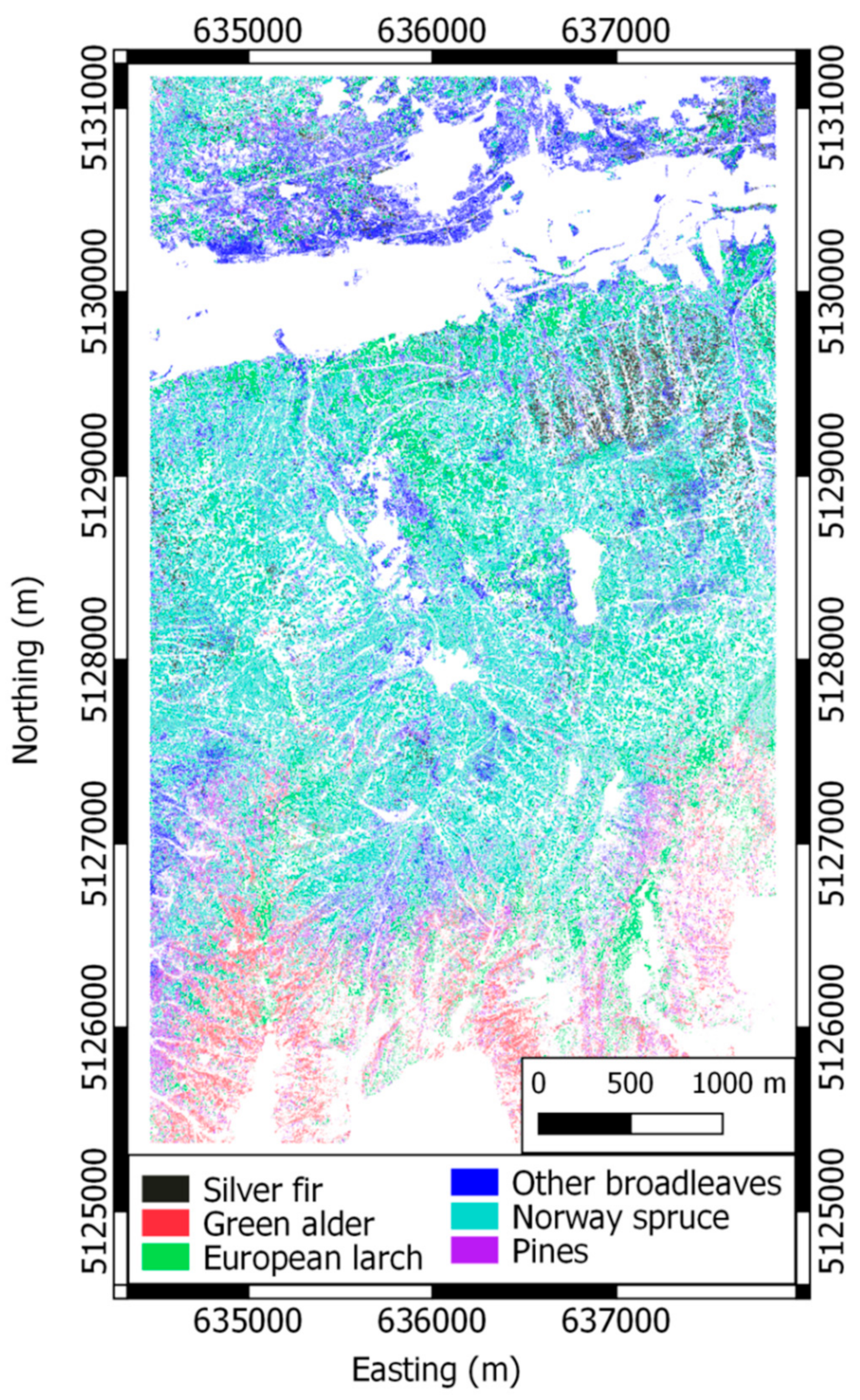
2.1.1. Dataset 1: Pellizzano

The Pellizzano study area (32 km²) is located in the municipality of Pellizzano (46°17’22″N, 10°46’05″E) in the Italian Alps (see Figure 1), and its altitude varies between 900 and 2200 m. Most of the total land area of the municipality is covered by productive forest, with a high number of different species, and patches of both pure and mixed tree species. The dominant species are Norway spruce (Picea abies (L.) H. Karst) that accounts for 65% of the total stem volume and European Larch (Larix decidua Mill.) with around 25%. The remaining 10% consists of other conifers, such as silver fir (Abies alba Mill.), Swiss stone pine (Pinus cembra L.), and some broadleaves such as silver birch (Betula pendula Roth), common alder (Alnus glutinosa (L.) Gaertn.), sycamore maple (Acer pseudoplatanus L.), and rowan (Sorbus aucuparia (L.) Crantz.).

The species, height, and locations of 5517 trees were collected in the summers of 2013 and 2014. However, the position and the species were only recorded for 3039 trees. These trees were located in the field across all the landscape, and the sampling was done in order to locate the largest number of species. The remaining trees were sampled inside 52 angle count sampling plots, and for these trees also the diameter at breast height and the height were measured. The height was measured by using a Haglöf Vertex hypsometer. For more information about the collection of the reference data, the reader is referred to [27]. Due to the low number of field samples for some species, the tree species were grouped into six classes: (i) sliver fir (199 trees); (ii) green alder (249 trees), (iii) European larch (1034 trees); (iv) other broadleaves (1150; all the broadleaves different from green alder), (v) Norway spruce (2553 trees); and (vi) pines (197 trees; Swiss stone pine, Scots pine, and Austrian pine).

Airborne LiDAR data were acquired between 7 and 9 September 2012, using a Riegl LMS-Q680i laser scanner (RIEGL Laser Measurement Systems GmbH, Horn, Austria). The scan frequency was 400 kHz, with a 60° field of view. Up to four returns per pulse were recorded, and the mean point density was approximately 48 pulses m⁻².

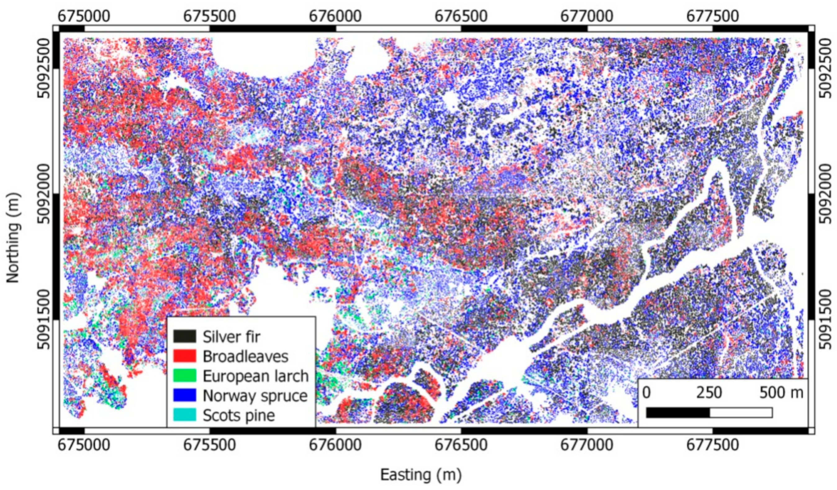
2.1.2. Dataset 2: Lavarone

The study area (4 km²) is located in the municipality of Lavarone (45°57’30.09″N, 11°16’25.17″E) in the Italian Alps (see Figure 1). The area has a complex structure that contains patches of mixed and pure species composition. The altitude varies from 1200 to 1600 m above the sea level. The dominant tree species are Norway spruce (Picea abies (L.) H. Karst.) at about 47% of the total stem volume, silver fir (Abies alba Mill.) at about 36%, and European beech (Fagus sylvatica L.) at about 13%. Other relevant species are European larch (Larix decidua Mill.) and Scots pine (Pinus sylvestris L.), which account for about 4%.

The species, height, and locations of 5655 trees were collected in the summers of 2016 and 2018. The field measurements of 2016 were done in 41 plots of 15 meters radius: the position, the species, and the DBH of 4812 trees were measured. The remaining trees (843) were measured in 2018, and they were sampled across all the landscape, and the sampling was done in order to locate the largest number of species. Due to the low number of field samples for some species, the tree species were grouped into five classes: (i) sliver fir (2164 trees); (ii) European larch (113 trees); (iii) broadleaves (1795 trees; all the broadleaves species), (iv) Norway spruce (1437 trees); and (v) Scots pine (146 trees).

LiDAR data were acquired by an Optech ALTM 3100EA sensor with a maximum scan angle of 21 degrees. The mean point density was 21.5 points per square meter for the first return, while the pulse density was 14.4 pulses m⁻². Up to four returns per pulse were measured.

2.2. LiDAR Data Preprocessing

The LiDAR point cloud was normalized to create a canopy height model (CHM) by subtracting the DTM from the z values of the LiDAR pulses. This operation was carried out by using the module lasground of the LAStools software (https://rapidlasso.com/). The intensity value of each LiDAR point was range-calibrated, using the following equation:

$$I_C=I*{\left(\frac{R}{Rs}\right)}^{\alpha }$$

(1)

where $I_C$ is the calibrated intensity, $I$ the raw intensity, $R$ is the sensor-to-target range, and $Rs$ is the reference range or average flying height. We considered an exponential factor $\alpha$ of 2.5 [10] since the environmental factors can be considered stable and the same acquisition parameters and instruments were maintained during the survey [28].

2.3. ITCs Delineation

The automatic ITCs delineation was performed by using the method implemented in the R package itcSegment and used in [27]. The algorithm follows three steps: (1) smoothing of the canopy height model: a Gaussian low-pass filter is applied to the rasterized CHM to smooth the surface and to reduce the number of potential local maxima; (2) local maxima extraction: a circular moving window of variable size is applied to the smoothed CHM to find a set of potential treetops (local maxima). A pixel of the CHM is labeled as local maxima if its value is greater than all other values in the window while being greater than some minimum height above ground. The window size is adapted according to the height of the central pixel of the window, which is predetermined in a user-defined look up table; (3) crown region growing: the algorithm iteratively searches for possible neighboring pixels to grow the crown of the tree around each local maxima. A pixel belongs to a specific region only if its vertical distance from the local maximum is less than a predefined percentage of the local maximum height, and less than a predefined maximum difference. The process repeats until no further pixel is added to any region. Once the region is fully grown, a 2D convex hull is applied, resulting in polygons that represent individual trees (ITCs).

To generate the reference ITCs dataset for species classification, a matching process between delineated ITCs and reference ground observations was applied. The adopted matching procedure followed two steps: (1) candidate search: all ground reference trees falling inside an ITC were considered as matching candidates; (2) candidate vote: selected candidates were ranked by their difference in height with the delineated ITCs and their Euclidian distance to the local maxima. A distance metric D was estimated by considering both parameters to select the best candidate as follows:

$$D=\sqrt{{\left(x_{CAN}-x_{ITC}\right)}^2+{\left(y_{CAN}-y_{ITC}\right)}^2+w*{\left(h_{CAN}-h_{ITC}\right)}^2}$$

(2)

where $\left(x_{CAN}, y_{CAN}, h_{CAN}\right)$ and $\left(x_{ITC}, y_{ITC}, h_{ITC}\right)$ denote the locations and heights of the field measured trees and the delineated ITCs, respectively; and $w$ is the user-defined weight. Here, the value of $w$ is set as 0.5 [29].

The matched ITCs were divided into training and test sets that were defined in order to have similar distributions in terms of species, tree height, and spatial location. In

Table 1. Number of training and test ITCs for the Pellizzano and Lavarone datasets.

Dataset 1: Pellizzano			Dataset 2: Lavarone
Class Name	Training Set	Test Set	Class Name	Training Set	Test Set
Sliver fir	52	51	Sliver fir	232	231
Green alder	80	79	European larch	35	34
European larch	313	312	Broadleaves	108	108
Other broadleaves	343	343	Norway spruce	253	252
Norway spruce	697	696	Scots pine	37	36
Pines	56	56

, a summary of the training and test sets for the two datasets is presented.

2.4. Feature Extraction

From each delineated ITC, features were extracted in order to build the classification models. In particular, two sets of features were considered: (i) 46 elevation and intensity features derived directly from the LiDAR point cloud; and (ii) three topography features derived from the DTM. The features are summarized in

Table 2. Description of the extracted features. “Z” means that the feature was extracted from the elevation values of the LiDAR points; “I” means that the feature was extracted from the intensity values of the LiDAR points; “P” refers to the corresponding percentile; and “R” refers to the corresponding return number.

Metric	Description
Zmax	Maximum Z
Zmean	Mean Z
Zsd	Standard deviation of Z distribution
Zskew	Skewness of Z distribution
Zkurt	Kurtosis of Z distribution
Zentropy	Entropy of Z distribution
ZqP	Ph percentile of height distribution, with P from 5 to 95 at steps of 5
ZpcumP	Cumulative percentage of points in the Pth layer, with P from 5 to 95 at steps of 5
Itot	Sum of intensities for each return
Imax	Maximum intensity
Imean	Mean intensity
Isd	Standard deviation of intensity
Iskew	Skewness of intensity distribution
Ikurt	Kurtosis of intensity distribution
IpcumzqP	Percentage of intensity returned below the Pth percentile of Z, with P from 5 to 95
pRth	Percentage of Rth return, with R from 1 to 4
Slope	Properties of the tangent plane to the surface
DTM	Digital terrain model value (m)
aspect	Compass direction in which the slope faces to

.

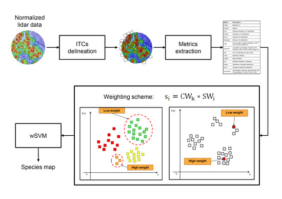
3. Proposed Weighted SVM-Based Approach for Tree Species Classification

In the recent years, SVM has been widely applied to classification problems in forestry applications [22]. In the standard SVM, all training samples have equal importance, and thus in the case of incomplete (poor) training sets (those with mislabeled imbalanced training samples), which are common in tree species classification, this may result in reduced classification performances. In this paper, we present a wSVM-based approach that weights the training samples in order to overcome such problems. Let S = ${\left\{(x_{\mathrm{i}},{\mathrm{y}}_{\mathrm{i}},{\mathrm{s}}_{\mathrm{i}})\right\}}_{\mathrm{i}=1}^{\mathrm{N}}$ be a set of labeled training samples, where $x_{\mathrm{i}}$ is the i-th training sample, ${\mathrm{y}}_{\mathrm{i}}$ is the corresponding class label from a pool of classes $K=k_1,\dots ,k_{\Psi }$, and ${\mathrm{s}}_{\mathrm{i}}$ is its weight. Then, in the wSVM, the optimization problem is defined as follows:

$$\begin{gathered} \frac{1}{2}{\left|\left|\mathrm{w}\right|\right|}_2^2+\mathrm{C}{\displaystyle \sum }_{\mathrm{i}=1}^{\mathrm{N}}{\mathrm{s}}_{\mathrm{i}}{\mathsf{\xi }}_{\mathrm{i}} \\ \mathrm{subject}\mathrm{to}:\left\{\begin{array}{c}{\mathrm{y}}_{\mathrm{i}}\left(\mathsf{\omega }.\Phi \left({\mathrm{x}}_{\mathrm{i}}\right)+\mathrm{b}\right)\ge 1-{\mathsf{\xi }}_{\mathrm{i}}\\ {\mathsf{\xi }}_{\mathrm{i}}\ge 0, \mathrm{i}=1,\dots ,\mathrm{i}\end{array}\right. \end{gathered}$$

(3)

where $\Phi ()$ is the mapping function that projects the samples from the original feature space to a higher dimensional space, and $\mathrm{b}$ is the bias. C is a regularization (i.e., penalty) parameter. From Equation (3), it can be seen that, in the wSVM, the penalty value C of misclassification for each training sample has a different weighting effect that is driven by ${\mathrm{s}}_{\mathrm{i}}$. A possible solution in the case of imbalanced classes in tree species classification problems is to allow a different penalty parameter for each tree species class. Specifically, samples of each class can be associated with different penalty values defined by class weights, so that the decision boundary can pay more attention to the minority classes.

The sample weight, ${\mathrm{s}}_{\mathrm{i}}$, could be defined by two components: a component dealing with the importance of the sample in describing the class distribution to which it belongs (which is called as intraclass weight) and a second component related to the importance to give to that specific class (which is called as interclass weight). Given this assumption, ${\mathrm{s}}_{\mathrm{i}}$ is formulated as follows:

$${\mathrm{s}}_{\mathrm{i}}={\mathrm{CW}}_{\mathrm{k}}*{\mathrm{SW}}_{\mathrm{i}}$$

(4)

where ${\mathrm{CW}}_{\mathrm{k}}$ is the interclass weight for the class k to which the sample ${\mathrm{x}}_{\mathrm{i}}$ belongs to, and ${\mathrm{SW}}_{\mathrm{i}}$ is the intraclass weight of the sample ${\mathrm{x}}_{\mathrm{i}}$. It is worth noting that the reason to have two components to define a weight, ${\mathrm{s}}_{\mathrm{i}},$ is to jointly consider the imbalanced class problem and the presence of mislabeled samples.

3.1. Interclass Weight

For a training set that has $\Psi$ classes, we propose to define the interclass weight ${\mathrm{CW}}_{\mathrm{k}}$ as follows:

$$C{W}_k=\frac{\max \left(N_k\right)}{N_k},k=1,\dots ,\mathit{\Psi }$$

(5)

where $N_k$ is the number of samples that belong to the k-th class. When this ratio is very large, we can lose information associated with the majority classes. This problem can be addressed by setting the class weight of majority classes as follows:

$$C{W}_{major}=mean\left(C{W}_k\right)$$

(6)

3.2. Intraclass Weight

To define the intraclass weights, we consider that training samples associated with the highest density regions of the feature space are much more important than those located in the low-density regions. This assumption is based on the fact that (i) samples in high-density regions are statistically very representative of the underlying class distribution, and (ii) the classification results on samples located in the high density patterns of the feature space affect more the overall accuracy of the classification process than those obtained on samples within low-density regions. Thus, we describe two approaches that define higher weights for the samples located in the high-density regions of the feature space, while giving reduced weights to those that fall into the low-density regions of the feature space. The first approach is based on k-means clustering and uses only the training samples, whereas the second approach is based on the mean distance among the samples and exploits a set of unlabeled samples.

3.2.1. Intraclass Weight Based on k-Means Clustering

In this approach, the training samples of each class are initially divided into $G$ clusters. Then, the density of each cluster is used to estimate the density of the samples in the feature space. If most of the training samples associated to the same class are grouped into one cluster, while the remaining samples are sparsely distributed, the training samples located in that cluster are considered much more reliable than those in the other clusters. Hence, higher weights are assigned to the samples located in the clusters characterized by a higher number of samples. The proposed approach can be summarized as follows:

• The k-means clustering is applied to the samples of each class in the training set independently from the samples of other classes to identify a set $\mathsf{\Omega }=\left\{c_1,c_2,\dots ,c_G\right\}$ of G-clusters. The number $G$ of clusters is defined as the square root of the half of the total number of samples in that class (as suggested in [30]);
• For each cluster $c_i$, a weight is determined as the number of samples located in that cluster. In this way, labeled samples that fall into the high-density clusters are more important for the classification problem and vice versa;
• Weights are normalized in the interval $\left[0,1\right]$.

These three operations are repeated for each class.

3.2.2. Intraclass Weight Based on Unlabeled Data

In this approach, the importance of each training sample is defined according to the distribution of the unlabeled samples. We assume that the importance of each training sample depends on its density in the feature space, i.e., training samples associated with the highest-density regions of the feature space are much more important than those located in the low-density regions. Thus, samples located in the high-density regions of the feature space are associated with the higher weights, while those that fall into the low-density regions of the feature space are associated to the lower weights. In this paper, unlabeled samples are associated to ITCs automatically delineated for which features have been extracted from LiDAR data but that were not matched with any field measured tree. The proposed approach aims at measuring the density $d_i$ of the unlabeled samples around the training sample $x_{\mathrm{i}}$ in the feature space. The density $d_i$ is estimated by considering the mean Euclidean distance of the training sample $x_{\mathrm{i}}$ to the P-nearest neighbour samples. By this way, a high-density region is considered as a region of the feature space where the mean Euclidean distance among the samples is small. The proposed approach for the estimation of sample weights can be summarized as follows:

• The Euclidean distance between each training sample and all the available unlabeled samples is computed;
• The mean value of the distance between each training sample $x_{\mathrm{i}}$ and the $P$ nearest unlabeled samples in the feature space is computed. The value of P varies depending on the class and is estimated as the square root of the total number of samples of each class in the training set;
• Weights are assigned according to the mean distance calculated during step 2: a small distance is related to the fact that the density around that sample is high, and thus a high value of the weight is assigned to that sample;
• Weights are normalized in the range $\left[0,1\right]$.

4. Results

4.1. Design of Experiments

The classification accuracy was assessed for both datasets in terms of overall accuracy (OA), kappa accuracy (KA), mean class accuracy (MCA), and producer’s accuracy (PA). The MCA was computed as the mean value of the PAs. Four classifiers were tested: (i) a standard $SVM$; (ii) a wSVM with only interclass weights ($wSV{M}^{CW}$); (iii) a wSVM with interclass weights and intraclass weights based on k-means clustering ($wSV{M}^{kmeans}$); and (iv) a wSVM with interclass weights and intraclass weights based on unlabeled data ($wSV{M}^{Uneighbor}$). For each classifier, we also provided the computational time (in seconds) required to train the classifier. The standard SVM and the wSVM classifiers used were the ones implemented in R in the package locClass [31]. In both cases, we used a radial basis kernel function (RBF), and the one-against-one multiclass strategy. The algorithms for the computation of the sample weights were implemented in R. The model selection for all considered classifiers was based on a grid-searching method: the values considered for the kernel width ranged from $2^{-5}$ to $2^5$ (11 values), while the values for the cost parameter C ranged from 1 to 128 (8 values).

To validate the robustness of the $wSV{M}^{kmeans}$ classifier compared to the standard $SVM$, wrongly labeled samples were added to the training set in order to observe the classification performance of each classifier. Those wrongly labeled samples were randomly taken from the pool of the unlabeled samples, and random labels were assigned among the classes considered in each dataset. The maximum number of wrongly labeled samples added to the original training set was set as one-third of the total training samples. In particular, we added a maximum of 500 and 200 wrongly labeled samples for Pellizzano and Lavarone, respectively. To ensure the distribution of classes in the training set was not changed, the proportion of samples belonging to each class was kept the same as in the training set. The number of wrongly labeled samples added to the training set started from 20 and increased by 20 at each iteration, until it reached the maximum. Since the procedure of adding wrongly labeled samples was a random process, each iteration was repeated 100 times, and the average accuracy is given in the results.

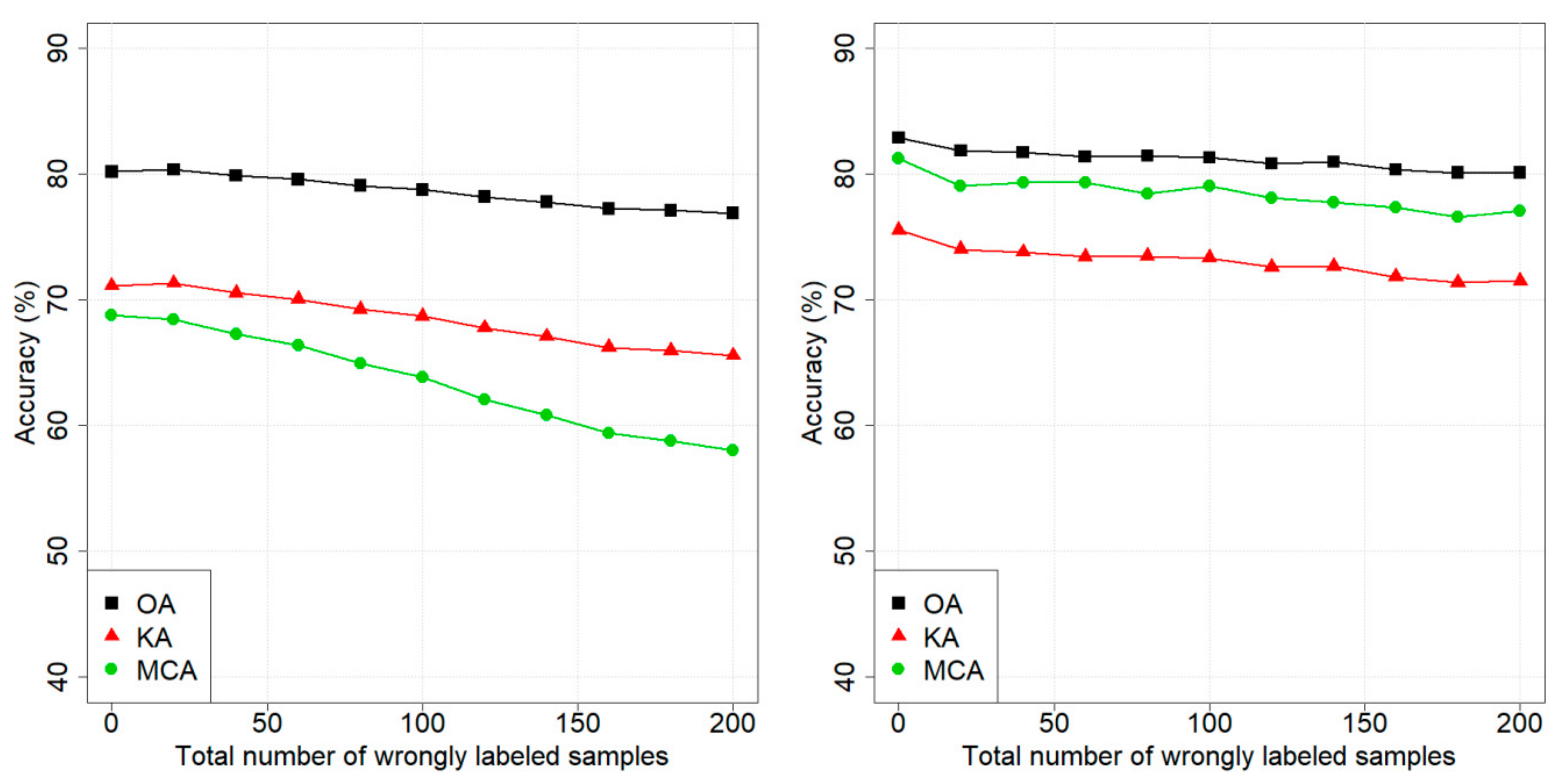
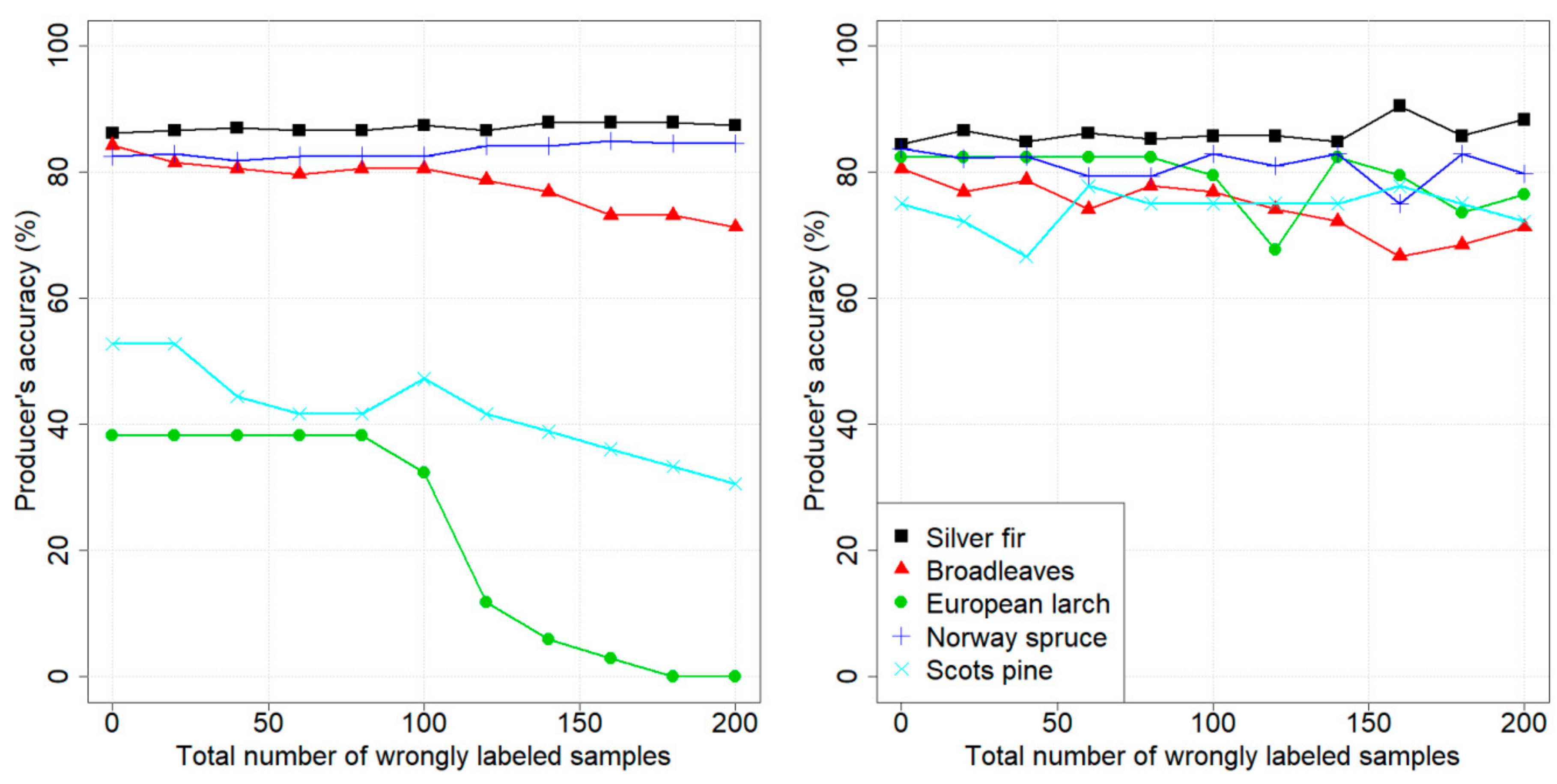
4.2. Dataset 1: Pellizzano

Table 3. Pellizzano dataset: overall classification accuracies (in %) and processing time (in seconds) of the different classifiers.

Classifier	OA	MCA	KA	Processing Time
$SVM$	79.2	62.2	69.2	57.96
$wSV{M}^{CW}$	80.7	71.4	72.1	60.70
$wSV{M}^{kmeans}$	79.1	72.9	70.2	58.25
$wSV{M}^{Uneighbor}$	80.8	71.5	72.4	898.87

reports the classification accuracies obtained by the four classifiers considered on the Pellizzano dataset. The $wSVMs$ classifiers provided higher accuracies compared to the standard $SVM$ classifier, particularly with the KA and the MCA. The most significant improvement was on the MCA, as it increased from 62.2%, using the standard $SVM$, to an average of 72%, using the $wSVMs$ classifiers. This increase in MCA was mainly due to the increase of PAs of the minority classes (i.e., silver fir and pines). The use of the $wSV{M}^{Uneighbor}$ slightly increased the MCA with respect to the $wSV{M}^{CW}$, while $wSV{M}^{kmeans}$ improved MCA with 1.5% compared to $wSV{M}^{CW}$. Regarding the computational time, it can be seen that there were no big differences between the processing time of the standard $SVM$ classifier, the $wSV{M}^{CW}$, and the $wSV{M}^{kmeans}$ classifiers. In contrast, the $wSV{M}^{Uneighbor}$ required an order of magnitude higher processing time compared to the standard $SVM$.

In

Table 4. Pellizzano dataset: producer’s accuracy for each class.

Classifier	Sliver Fir	Green Alder	European Larch	Other Broadleaves	Norway Spruce	Pines
$SVM$	5.9	91.1	67.9	82.8	89.9	35.7
$wSV{M}^{CW}$	39.2	94.9	68.6	83.7	88.2	53.6
$wSV{M}^{kmeans}$	47.1	93.7	68.3	84.0	83.6	60.7
$wSV{M}^{Uneighbor}$	39.2	93.7	71.2	84.5	87.1	53.6

, the PAs for each class are presented. Using the $wSV{M}^{CW}$ classifier, the classification accuracy of the minority classes significantly improved compared to that obtained by the standard $SVM$: for sliver fir class, the PA increased from 5.9% to 39.2%, and for pines class, the PA increased from 35.7% to 53.6%. For the other four classes, the $wSV{M}^{CW}$ provided better results than the standard $SVM$ except for the Norway spruce (its producer’s accuracy decreased of 1.7%). Comparing the performance of $wSV{M}^{kmeans}$ classifier with the performance of $wSV{M}^{CW}$ classifier, the accuracies on minority classes improved significantly: 7.8% for sliver fir and 7.1% for pines. PA of European larch and the other broadleaves did not show any large change, while Norway spruce PA decreased by 4.6%. Considering the $wSV{M}^{Uneighbor}$ classifier, the performances on all classes were very similar to the ones of the $wSV{M}^{CW}$. In general, the performances of the $wSVMs$ classifiers were good since the majority classes (Norway spruce and other broadleaves) still achieved high accuracies (over 80%), while the minority classes (silver fir and pines) experienced a significant improvement. Looking at the confusion matrices (

Table 5. Pellizzano dataset: confusion matrices on the test set for the considered classifiers. SF = silver fir. GA = green alder. EL = European larch. OB = other broadleaves. NS = Norway spruce. P = Pine.

$\mathit{S}\mathit{V}\mathit{M}$	SF	GA	EL	OB	NS	P	$\mathit{w}\mathit{S}\mathit{V}{\mathit{M}}^{\mathit{C}\mathit{W}}$	SF	GA	EL	OB	NS	P
SF	3	0	0	1	0	2	SF	20	0	6	7	19	3
GA	0	72	0	4	0	0	GA	0	75	2	4	1	1
EL	5	0	212	15	33	23	EL	3	0	214	12	28	11
OB	5	6	16	284	36	8	OB	3	3	16	287	30	9
NS	38	1	81	37	626	3	NS	24	1	66	25	614	2
P	0	0	3	2	1	20	P	1	0	8	8	4	30
$\mathit{w}\mathit{S}\mathit{V}{\mathit{M}}^{\mathit{k}\mathit{m}\mathit{e}\mathit{a}\mathit{n}\mathit{s}}$	SF	GA	EL	OB	NS	P	$\mathit{w}\mathit{S}\mathit{V}{\mathit{M}}^{\mathit{U}\mathit{n}\mathit{e}\mathit{i}\mathit{g}\mathit{h}\mathit{b}\mathit{o}\mathit{r}}$	SF	GA	EL	OB	NS	P
SF	24	0	7	9	24	3	SF	20	0	3	5	14	3
GA	0	74	2	5	0	1	GA	0	74	1	4	0	0
EL	6	0	213	11	45	10	EL	5	0	222	15	36	12
OB	3	3	20	288	37	8	OB	3	4	17	290	36	9
NS	17	1	61	22	582	0	NS	22	1	61	22	606	2
P	1	1	9	8	8	34	P	1	0	8	7	4	30

), we can see that silver fir and European larch are mainly mixing with Norway spruce, while the pines are mainly mixing with the European larch. Regarding the broadleaves, we can see that the green alder has few samples confused with the other broadleaves, while the other broadleaves are mixing mainly with Norway spruce and European larch.

Figure 2 illustrates the results of adding wrongly labeled samples to the training set for the standard $SVM$ and $wSV{M}^{kmeans}$. In the case of the standard $SVM$ classifier, all three accuracy metrics (i.e., OA, KA, and MCA) decreased when the number of wrongly labeled samples in the training set was increased. Considering the $wSV{M}^{kmeans}$ the accuracies remained high, even with a high number of wrongly labeled samples in the training set. As an example, with 500 added wrongly labeled samples, the difference in OA and KA between the standard $SVM$ and the $wSV{M}^{kmeans}$ was approximately 3%, while the difference in MCA was around 5%.

To investigate how the wrongly labeled samples affect the PA of each class, Figure 3 illustrates the variation in PAs values, using the standard $SVM$ and the $wSV{M}^{k-means}$ classifiers, while adding wrongly labeled samples to the training set. In the case of the $wSV{M}^{k-means}$ classifier, it can be seen that the PAs values did not have any remarkable change compared to the starting case (when zero wrongly labeled samples added). The PAs of the two minority classes fluctuated, but they were always above 40%, even at the last step of the experiment. The behavior was opposite in the case of the standard $SVM$ classifier: while the PAs of majority classes remained stable, the PAs of minority classes decreased to 0%.

Figure 4 shows the classification map for the Pellizzano area obtained using the $wSV{M}^{kmeans}$. It can be seen that, in Pellizzano, tree species are localized in different areas. In the northern part of the study site, the dominant tree species are broadleaves, in the middle of the area there is mainly Norway spruce, while in the southern part (that is also the one at the highest altitude) there are mainly European larch and green alder.

4.3. Dataset 2: Lavarone

The results on the Lavarone dataset are quite similar to the ones of the Pellizzano dataset. Compared to the standard $SVM$ classifier, the $wSV{M}^{kmeans}$ increased the OA of 2.7%, and the KA of 4.4%, while $wSV{M}^{Uneighbor}$ obtained similar results as $wSV{M}^{kmeans}$ (see

Table 6. Lavarone dataset: classification accuracies and processing time of the different classifiers.

Classifiers	OA	MCA	Kappa	Processing Time (s)
$SVM$	80.2	68.8	71.1	20.86
$wSV{M}^{CW}$	81.4	77.8	73.5	19.72
$wSV{M}^{kmeans}$	82.9	81.2	75.5	21.49
$wSV{M}^{Uneighbor}$	82.6	76.9	74.9	530.75

). By using the $wSV{M}^{CW}$ classifier, the MCA increased from 68.8% to 77.8%, while by using the $wSV{M}^{kmeans}$, it reached 81.2%, and using the $wSV{M}^{Uneighbor},$ it reached 76.9%. In general, compared to the standard $SVM$, $wSVM$ classifiers increased the accuracy by approximately 12%. Regarding the computational time, as in the case of Pellizzano, only the $wSV{M}^{Uneighbor}$ had computational time in a different order of magnitude than the other three classifiers.

European larch and Scots pine (that are minority classes in this dataset) were not properly classified by the standard $SVM$ (

Table 7. Lavarone dataset: producer’s accuracy for each class.

Classifiers	Sliver Fir	Broadleaves	European Larch	Norway Spruce	Scots Pine
$SVM$	86.1	84.3	38.2	82.5	52.8
$wSV{M}^{CW}$	87.0	78.7	73.5	80.2	69.4
$wSV{M}^{kmeans}$	84.4	80.6	82.4	83.7	75.0
$wSV{M}^{Uneighbor}$	87.9	78.7	67.6	83.7	66.7

). While using the $wSV{M}^{CW}$ classifier, their PAs improved significantly: 35.3% for European larch and 16.7% for Scots pine. On the other hand, the accuracy of the broadleaves class decreased by 5.6% by using $wSV{M}^{CW}$.

By comparing the performances of the two $wSVM$ classifiers based on both intraclass and interclass sample weights ($wSV{M}^{kmeans}$ and $wSV{M}^{Uneighbor}$) with the $wSV{M}^{CW}$ classifier, it can be seen that there was not a significant improvement by using the $wSV{M}^{Uneighbor}$ classifier, while with the $wSV{M}^{kmeans}$ classifier, the accuracies were higher in most of the cases. In greater detail, the PA of European larch gained nearly 9%, reaching to 82.4%. This accuracy was equal to the classification accuracy of the majority classes. Scots pine also achieved a sharp increase to 75% compared to 69.4% obtained by the $wSV{M}^{CW}$ classifier. The confusion matrices (

Table 8. Lavarone dataset: confusion matrices on the test set for the considered classifiers. SF = silver fir. B = broadleaves. EL = European larch. NS = Norway spruce. SP = Scots pine.

$\mathit{S}\mathit{V}\mathit{M}$	SF	B	EL	NS	SP	$\mathit{w}\mathit{S}\mathit{V}{\mathit{M}}^{\mathit{C}\mathit{W}}$	SF	B	EL	NS	SP
SF	199	9	0	28	0	SF	201	12	1	23	0
B	3	91	2	8	2	B	4	85	0	8	2
EL	0	1	13	2	0	EL	2	2	25	11	1
NS	28	7	18	208	15	NS	23	7	7	202	8
SP	1	0	1	6	19	SP	1	2	1	8	25
$\mathit{w}\mathit{S}\mathit{V}{\mathit{M}}^{\mathit{k}\mathit{m}\mathit{e}\mathit{a}\mathit{n}\mathit{s}}$	SF	B	EL	NS	SP	$\mathit{w}\mathit{S}\mathit{V}{\mathit{M}}^{\mathit{U}\mathit{n}\mathit{e}\mathit{i}\mathit{g}\mathit{h}\mathit{b}\mathit{o}\mathit{r}}$	SF	B	EL	NS	SP
SF	195	7	0	19	0	SF	203	13	0	23	0
B	4	87	0	8	1	B	4	85	0	8	1
EL	1	3	28	7	0	EL	0	2	23	5	0
NS	31	11	5	211	8	NS	24	7	10	211	11
SP	0	0	1	7	27	SP	0	1	1	5	24

) showed that silver fir and European larch were mainly mixing with Norway spruce, and, similarly, Norway spruce was mainly mixing with silver fir.

Figure 5 shows the results obtained by adding wrongly labeled samples to the training set. As it can be seen, the $wSV{M}^{kmeans}$ classifier is more robust to noise compared to the standard $SVM$. In greater detail, when 200 wrongly labeled samples were added, the decrease in OA was 3.3% for the standard $SVM$ and 2.8% for the $wSV{M}^{kmeans}$; for MCA, the decrease was by 10.8% and 4.2%, and for KA, it was by 5.6% and 4.1%.

Figure 6 illustrates the variation in PAs values by using the standard $SVM$ and the $wSV{M}^{kmeans}$ classifiers, while adding wrongly labeled samples in the training set. In the case of the $wSV{M}^{kmeans}$ classifier, it can be seen that all the classes reached a PA higher than 60%, and they did not seem particularly affected by the presence of wrongly labeled samples. In contrast, in the case of the standard $SVM$ classifier, like in Pellizzano, the PAs of minority classes remarkably decreased. For European larch, the accuracy decreased from 39% to 0%, meaning that no tree of this class could be detected anymore, while for Scots pine, the PA decreased from around 52% to approximately 35%, when 200 wrongly labeled samples were added.

The classification map of Lavarone, using the $wSV{M}^{kmeans}$, classifier is shown in Figure 7. As it can be seen, Norway spruce and sliver fir are concentrated in the western part of the area, while broadleaves mainly grow in the eastern part of the area. Minority classes are sparsely distributed over the area.

5. Discussion

In this study, a wSVM-based approach for tree species classification at ITC level, using LiDAR data, was presented. In the proposed approach, the wSVM weights of the training samples are assigned in order to reach two objectives: (i) to reduce the effect of the imbalanced distribution of the classes in the training set; and (ii) to reflect the importance level of each training sample in order to reduce the effect of wrongly labeled samples.

Regarding the problem of the imbalance class distribution in the training set in tree species classification, our study provides a possible solution by assigning different class weights to different classes. Indeed, with the proposed weights, all the minority species in both datasets analyzed experienced an increase in classification accuracy. In particular, for coniferous species having a small number of training samples, the improvement was significant compared to the results achieved with a standard supervised SVM (Table 4 and Table 7). Using the proposed wSVM-based approach, the accuracy of majority species remained generally stable, with some cases where there was a slight decrease, while minority species experienced a high gain in accuracy. It is worth noting that there should exist a tradeoff among minority and majority classes in order to achieve the target of the classification. Since wSVM assigns different weights to different classes (or samples), it forces the new separating hyperplane to pay more attention on the minority classes samples, thus leading to a misclassification of some majority classes samples. In our specific cases, Norway spruce experienced a slight decrease, and, even though it remained over 80%, this can represent a problem, as it is the dominant species in the analyzed areas, which accounts for half of the total stem volume. Thus, the weighting scheme should be adjusted by the user depending on its target.

The effectiveness of the wSVM-based approach with respect to the standard SVM for the improvement of the classification accuracy on the minority species is related to two main reasons: (i) as a result of using interclass weights, class imbalance problems are significantly diminished; and (ii) as a results of using intraclass weights, the effect of wrongly labeled samples to contribute to the definition of the SVM hyperplane is reduced.

Regarding the presence of wrongly labeled samples in the training set, we showed that the proposed approach is effective in dealing with them. For both datasets, the wSVM approach was better at dealing with the presence of wrongly labeled samples than the standard one. As an example, in the Pellizzano dataset, after adding 200 wrongly labeled samples to the training set, the supervised SVM could not detect minority classes anymore, while the proposed wSVM was able to keep the accuracies stable. This is a great advantage in tree species classification since the process of field data collection could have many sources of errors due to positioning accuracy, but also to the ITCs delineation and to the matching procedure among ITCs and field data.

Despite the classification performances, two other important criteria should be considered when evaluating a new classifier: (i) the number of parameters to be tuned and (ii) the processing time of the classifier. Regarding the number of parameters, the proposed approach based on wSVM and intraclass weights requires one additional parameter compared to a standard SVM. For $wSV{M}^{Uneighbor}$, the additional parameter is the number, $U$, of nearest neighboring samples for each training sample to consider in the computation of the distance. For the $wSV{M}^{kmeans}$, the additional parameter is the number of clusters in which to divide the training samples of each class. In our experiments with $wSV{M}^{Uneighbor},$ we noticed that there is not a significant change in classification accuracy when varying $U$. This could be explained by the fact that, since we have many unlabeled samples (about 475,000 for Pellizzano and 100,000 for Lavarone) in both datasets, the distances between the samples will be not too different, and thus the sample weights may not work effectively. In the case of $wSV{M}^{kmeans}$, $G$ is defined as the square root of the half of the total number of samples in that class, as in [30]. During our experiments, we varied $G$, and we noticed that the value of $G$ defined by that equation allowed us to have among the best classification results.

The high computational time required for the training of the $wSV{M}^{Uneighbor}$ is related to the number of unlabeled samples. Indeed, the $wSV{M}^{Uneighbor}$ classifier, in order to obtain a weight for each training sample, has to calculate the distance in the feature space between each training sample and each sample in the pool of the unlabeled set. Then the mean distance between the sample and the $U$ nearest neighbors is determined. Thus, if the number of unlabeled samples is large, this process requires a long time to complete. The processing time can be reduced by reducing the number of the considered unlabeled samples. This process can be done by randomly sampling the unlabeled set to get the desired number of samples. However, as a tradeoff, the quality of the subset of unlabeled set might not be guaranteed. Considering the two datasets analyzed, from previous forest inventories, we know that both areas have minority classes that account for less than 5% of the total stem volume. If the subset of the unlabeled set contains only majority samples, the distance between each minority training sample to the unlabeled samples becomes larger compared to the majority training samples, and thus the weight of each minority training sample becomes small and such classes are penalized.

The main limitation of the proposed wSVM approach with respect to a standard approach based on SVM is that the weighting algorithms will perform well associated to the samples located in the high-density regions of the feature space, thus on trees with characteristics similar to the ones of the other members of that species, while it will probably penalize samples that are quite different from other samples of the same class. This could actually happen in tree species classification, as there could be trees that, for reasons related to health, age, or soil properties, grow quite differently compared to the other trees of the same species in the same area. This should be taken into consideration when applying the proposed approach, particularly if it is known that, in the considered area, there are anomalies among the trees of the same species.

A last finding of this study is that LiDAR data could be used to classify tree species in temperate forests. In the literature, good results have been obtained in boreal forests [12], where the species diversity is quite low (usually only three tree species are considered in this biome). In this study, we obtained good results for distinguishing the main tree species groups that are present in the Alps (PAs over 70%), opening up the possibility to have broad species classifications with high spatial accuracy in this area, using already available data. Indeed, in Europe, nowadays, many counties and countries have full coverage of LiDAR data for hydrogeological purposes, and these data could also be used for a species coverage map. The classification errors that we found are mainly related to the limitations of the features extracted from LiDAR data: silver fir is mainly confused with Norway spruce, and the same is happening for European larch. These three tree species have quite a similar shape, as well as similar reflectance in the near-infrared, where the LiDAR intensity features are located. For the same reason, it was not possible to distinguish among the different broadleaf species, except for the green alder, which has a very different mean height compared to the other species. From an operational viewpoint, this does not represent much of a problem, as the majority of the stem volume in the Alps is in conifer species, and the commercial timber is also mainly derived from conifers. On the other hand, if the focus is on biodiversity studies, this represents a limitation. In this case, we can expect that the use of the new multispectral LiDAR sensors [32] could improve the results, opening up new possibilities for studies on tree species classification from LiDAR data.

By comparing the results obtained in this study with similar studies in the literature, we can find both differences and similarities. First of all, considering the features used in the classification process, many studies used similar features to the ones used by us (e.g., [12,14,15,16,18,33]), while others used 3D features (e.g., [17,19]) or bi-temporal LiDAR features (e.g., [8,21]). By looking in detail at the ones that used features similar to the ones in this study it is possible to see that some studies used exactly the same features as us (e.g., [12,14,16]), while others added additional features extracted from the 3D information (e.g., [15,18,33]). In terms of classifiers, almost every study tested different classifiers: support-vector-machine-based classifiers (e.g., [18,19,33]), linear discriminant analysis (e.g., [12,14,15,16]), random forest (e.g., [12,17]), and k-nearest neighbor and k-most-similar neighbor (e.g., [12]). The tree species also change in each study, as they are related to the type of analyzed forest. By considering the species that are also present in our datasets, we can see that Norway spruce, pines, and broadleaves are usually quite well separated in all the studies, with accuracies above 80%. Lower accuracies are obtained for separating individual broadleaves species, like in the study of Brandtberg [21], where three broadleaf species were classified with an accuracy of 64%.

6. Conclusions

In this study, a wSVM-based approach for tree species classification at ITC level, using LiDAR data, was presented. The proposed weighting schemes for use in a wSVM method proved to be effective in dealing with two main problems of the reference data in tree species classification: (i) imbalanced classes distribution and (ii) the presence of wrongly labeled training samples. In both datasets considered, the improvement of the proposed approach with respect to a standard SVM classifier was significant for the underrepresented classes. Moreover, in this study, we showed that the proposed approach, combined with features extracted from LiDAR data, could be used to classify the main tree species of temperate forests, opening new possibilities for future applications of LiDAR data.

As future development of this work, it can be interesting to use the proposed approach for other data types, like hyperspectral and multispectral data, to further evaluate their effectiveness. Further development could be to test these methods in connection with transfer-learning algorithms, in order to use training data in one area to classify data in other areas acquired in other moments in time. Moreover, it could be interesting to apply similar approaches to the prediction of ITC level biomass, and tree diameters.

References

1. Tabacchi, G.; Di Cosmo, L.; Gasparini, P. Aboveground tree volume and phytomass prediction equations for forest species in Italy. Eur. J. For. Res. 2011, 130, 911–934. [Google Scholar] [CrossRef]
2. Dalponte, M.; Bruzzone, L.; Gianelle, D. Tree species classification in the Southern Alps based on the fusion of very high geometrical resolution multispectral/hyperspectral images and LiDAR data. Remote Sens. Environ. 2012, 123, 258–270. [Google Scholar] [CrossRef]
3. Heinzel, J.; Koch, B. Investigating multiple data sources for tree species classification in temperate forest and use for single tree delineation. Int. J. Appl. Earth Obs. Geoinf. 2012, 18, 101–110. [Google Scholar] [CrossRef]
4. Shang, X.; Chazette, P. Interest of a full-waveform flown UV lidar to derive forest vertical structures and aboveground carbon. Forests 2014, 5, 1454–1480. [Google Scholar] [CrossRef] [Green Version]
5. Graves, S.J.; Asner, G.P.; Martin, R.E.; Anderson, C.B.; Colgan, M.S.; Kalantari, L.; Bohlman, S.A. Tree Species Abundance Predictions in a Tropical Agricultural Landscape with a Supervised Classification Model and Imbalanced Data. Remote Sens. 2016, 8, 161. [Google Scholar] [CrossRef] [Green Version]
6. Dalponte, M.; Ørka, H.O.; Gobakken, T.; Gianelle, D.; Næsset, E. Tree species classification in boreal forests with hyperspectral data. IEEE Trans. Geosci. Remote Sens. 2013, 51, 2632–2645. [Google Scholar] [CrossRef]
7. Fassnacht, F.E.; Neumann, C.; Forster, M.; Buddenbaum, H.; Ghosh, A.; Clasen, A.; Joshi, P.K.; Koch, B. Comparison of Feature Reduction Algorithms for Classifying Tree Species with Hyperspectral Data on Three Central European Test Sites. IEEE J. Sel. Top. Appl. Earth Obs. Remote Sens. 2014, 7, 2547–2561. [Google Scholar] [CrossRef]
8. Kim, S.; McGaughey, R.J.; Andersen, H.-E.; Schreuder, G. Tree species differentiation using intensity data derived from leaf-on and leaf-off airborne laser scanner data. Remote Sens. Environ. 2009, 113, 1575–1586. [Google Scholar] [CrossRef]
9. Wasser, L.; Day, R.; Chasmer, L.; Taylor, A. Influence of Vegetation Structure on Lidar-derived Canopy Height and Fractional Cover in Forested Riparian Buffers During Leaf-Off and Leaf-On Conditions. PLoS ONE 2013, 8, e54776. [Google Scholar] [CrossRef] [Green Version]
10. Korpela, I.; Ørka, H.O.; Hyyppä, J.; Heikkinen, V.; Tokola, T. Range and AGC normalization in airborne discrete-return LiDAR intensity data for forest canopies. ISPRS J. Photogramm. Remote Sens. 2010, 65, 369–379. [Google Scholar] [CrossRef]
11. Hovi, A.; Korhonen, L.; Vauhkonen, J.; Korpela, I. LiDAR waveform features for tree species classification and their sensitivity to tree- and acquisition related parameters. Remote Sens. Environ. 2016, 173, 224–237. [Google Scholar] [CrossRef]
12. Korpela, I.; Ole Ørka, H.; Maltamo, M.; Tokola, T.; Hyyppä, J. Tree species classification using airborne LiDAR—Effects of stand and tree parameters, downsizing of training set, intensity normalization, and sensor type. Silva Fenn. 2010, 44, 319–339. [Google Scholar] [CrossRef] [Green Version]
13. Lin, C.; Thomson, G.; Popescu, S. An IPCC-Compliant Technique for Forest Carbon Stock Assessment Using Airborne LiDAR-Derived Tree Metrics and Competition Index. Remote Sens. 2016, 8, 528. [Google Scholar] [CrossRef] [Green Version]
14. Ørka, H.O.; Næsset, E.; Bollandsås, O.M. Classifying species of individual trees by intensity and structure features derived from airborne laser scanner data. Remote Sens. Environ. 2009, 113, 1163–1174. [Google Scholar] [CrossRef]
15. Li, J.; Hu, B.; Noland, T.L. Classification of tree species based on structural features derived from high density LiDAR data. Agric. For. Meteorol. 2013, 171–172, 104–114. [Google Scholar] [CrossRef]
16. Holmgren, J.; Persson, Å. Identifying species of individual trees using airborne laser scanner. Remote Sens. Environ. 2004, 90, 415–423. [Google Scholar] [CrossRef]
17. Ko, C.; Sohn, G.; Remmel, T.K. Tree genera classification with geometric features from high-density airborne LiDAR. Can. J. Remote Sens. 2013, 39, S73–S85. [Google Scholar] [CrossRef]
18. Vaughn, N.R.; Moskal, L.M.; Turnblom, E.C. Tree Species Detection Accuracies Using Discrete Point Lidar and Airborne Waveform Lidar. Remote Sens. 2012, 4, 377–403. [Google Scholar] [CrossRef] [Green Version]
19. Harikumar, A.; Bovolo, F.; Bruzzone, L. An Internal Crown Geometric Model for Conifer Species Classification with High-Density LiDAR Data. IEEE Trans. Geosci. Remote Sens. 2017, 55, 2924–2940. [Google Scholar] [CrossRef]
20. Kim, S.; Hinckley, T.; Briggs, D. Classifying individual tree genera using stepwise cluster analysis based on height and intensity metrics derived from airborne laser scanner data. Remote Sens. Environ. 2011, 115, 3329–3342. [Google Scholar] [CrossRef]
21. Brandtberg, T. Classifying individual tree species under leaf-off and leaf-on conditions using airborne lidar. ISPRS J. Photogramm. Remote Sens. 2007, 61, 325–340. [Google Scholar] [CrossRef]
22. Fassnacht, F.E.; Latifi, H.; Stereńczak, K.; Modzelewska, A.; Lefsky, M.; Waser, L.T.; Straub, C.; Ghosh, A. Review of studies on tree species classification from remotely sensed data. Remote Sens. Environ. 2016, 186, 64–87. [Google Scholar] [CrossRef]
23. Zhen, Z.; Quackenbush, L.; Zhang, L. Trends in Automatic Individual Tree Crown Detection and Delineation—Evolution of LiDAR Data. Remote Sens. 2016, 8, 333. [Google Scholar] [CrossRef] [Green Version]
24. Lindberg, E.; Holmgren, J. Individual Tree Crown Methods for 3D Data from Remote Sensing. Curr. For. Rep. 2017, 3, 19–31. [Google Scholar] [CrossRef] [Green Version]
25. Dalponte, M.; Ene, L.T.; Marconcini, M.; Gobakken, T.; Næsset, E. Semi-supervised SVM for individual tree crown species classification. ISPRS J. Photogramm. Remote Sens. 2015, 110, 77–87. [Google Scholar] [CrossRef]
26. Dalponte, M.; Ene, L.T.; Ørka, H.O.; Gobakken, T.; Næsset, E. Unsupervised Selection of Training Samples for Tree Species Classification Using Hyperspectral Data. IEEE J. Sel. Top. Appl. Earth Obs. Remote Sens. 2014, 7, 3560–3569. [Google Scholar] [CrossRef]
27. Dalponte, M.; Coomes, D.A. Tree-centric mapping of forest carbon density from airborne laser scanning and hyperspectral data. Methods Ecol. Evol. 2016, 7, 1236–1245. [Google Scholar] [CrossRef] [Green Version]
28. Yu, X.; Hyyppä, J.; Litkey, P.; Kaartinen, H.; Vastaranta, M.; Holopainen, M. Single-Sensor Solution to Tree Species Classification Using Multispectral Airborne Laser Scanning. Remote Sens. 2017, 9, 108. [Google Scholar] [CrossRef] [Green Version]
29. Zhao, K.; Suarez, J.C.; Garcia, M.; Hu, T.; Wang, C.; Londo, A. Utility of multitemporal lidar for forest and carbon monitoring: Tree growth, biomass dynamics, and carbon flux. Remote Sens. Environ. 2018, 204, 883–897. [Google Scholar] [CrossRef]
30. Demir, B.; Bruzzone, L. A multiple criteria active learning method for support vector regression. Pattern Recognit. 2014, 47, 2558–2567. [Google Scholar] [CrossRef]
31. Schiffner, J.; Hillebrand, S. schiffner/locClass: Collection of Local Classification Methods. 2017. Available online: https://rdrr.io/github/schiffner/locClass/ (accessed on 8 December 2019).
32. Dalponte, M.; Ene, L.; Gobakken, T.; Næsset, E.; Gianelle, D. Predicting Selected Forest Stand Characteristics with Multispectral ALS Data. Remote Sens. 2018, 10, 586. [Google Scholar] [CrossRef] [Green Version]
33. Lin, Y.; Hyyppä, J. A comprehensive but efficient framework of proposing and validating feature parameters from airborne LiDAR data for tree species classification. Int. J. Appl. Earth Obs. Geoinf. 2016, 46, 45–55. [Google Scholar] [CrossRef]
Figure 1. Location of the two considered study areas: (1) Pellizzano and (2) Lavarone. In the inset is the location of the Autonomous Province of Trento in Italy.
Remotesensing 11 02948 g001
Figure 2. Pellizzano dataset: performances of the S V M (left panel) and the w S V M k m e a n s (right panel) classifiers when wrongly labeled samples are added.
Remotesensing 11 02948 g002
Figure 3. Pellizzano dataset: variation of PA on each class, using S V M (left panel) and w S V M k m e a n s (right panel), adding wrongly labeled samples.
Remotesensing 11 02948 g003
Figure 4. Pellizzano dataset: ITCs classification map, using w S V M k m e a n s .
Remotesensing 11 02948 g004
Figure 5. Lavarone dataset: performances of the S V M (left panel) and the w S V M k m e a n s (right panel) classifiers when wrongly labeled samples are added.
Remotesensing 11 02948 g005
Figure 6. Lavarone dataset: variation of PA on each class, using S V M (left panel) and w S V M k m e a n s (right panel), adding wrongly labeled samples.
Remotesensing 11 02948 g006
Figure 7. Lavarone dataset: ITCs classification map, using w S V M k m e a n s .
Remotesensing 11 02948 g007