1. Introduction
Top-of-atmosphere (TOA) albedo is a crucial component of the energy budget of the Earth [
1,
2]. Estimation of TOA albedo from remote sensing data is a unique means to generate TOA albedo products at regional or global scales. Different algorithms have been proposed to estimate TOA albedo from satellite data, and multiple TOA albedo products from both broadband and narrowband sensors have been developed [
3,
4,
5,
6,
7,
8,
9,
10,
11,
12,
13,
14,
15,
16,
17], some of which have a relatively high spatial resolution that is helpful in studying the energy budget at regional scales [
15,
16,
17].
Currently, different researchers have used these products to analyze the Earth’s energy budget. For instance, numerous studies have attempted to calculate the Arctic energy budget based on the energy equation integrated over the atmospheric column using different reanalysis datasets [
18,
19,
20,
21,
22,
23]. TOA products based on satellite data were used to calculate the downward net radiative flux at the TOA because of their better accuracy than reanalysis datasets. In addition, several studies have used the Diagnosing Earth’s Energy Pathways in the Climate system (DEEP-C) products to calculate the surface energy budget [
24,
25,
26]. Smith et al. [
24] built upon the DEEP-C datasets by including estimates of the ocean heat content trends and developing a combined simulated/observation-based record of net downward TOA radiation extending back to 1960. Trenberth and Fasullo [
25] stated that the net flux of energy into the surface can be estimated when the net downward radiation at the TOA (which can be obtained from DEEP-C) is combined with atmospheric energy transport and its divergence. By employing net radiation at the TOA from DEEP-C, Mayer et al. [
26] further refined estimates of the net surface energy flux based on this method.
To ensure these products are more effectively used, it is necessary to evaluate them. Unlike ground-based parameters, the TOA albedo products cannot be validated by direct comparison to in situ measurements. The quality of different data records can only be evaluated by intercomparison to other products [
27]. In addition to the widely used Clouds and the Earth’s Radiant Energy System (CERES) product, there are multiple TOA albedo satellite products available from different satellite observations using different estimation algorithms. For instance, Wang and Liang [
15] have developed TOA albedo products over land based on Moderate Resolution Imaging Spectroradiometer (MODIS) data (TAL-MODIS) and compared them to CERES data. Urbain et al. [
16] released the Climate Monitoring Satellite Application Facility (CM SAF) TOA radiation MVIRI/SEVIRI data record and made intercomparisons to the CERES data. Song et al. [
17] developed a long-term record of TOA albedo over land from Advanced Very High Resolution Radiometer (AVHRR) data (TAL-AVHRR) and compared it to both CM SAF and CERES data. However, no study has systematically compared all five products. In this study, the five TOA albedo products were comprehensively intercompared to demonstrate their differences.
The organization of this paper is as follows.
Section 2 introduces the CERES, TAL-AVHRR, TAL-MODIS, CM SAF, and DEEP-C TOA albedo products. Data processing methods are also described in this section. The results of the differences between the five products and the corresponding analysis are presented in
Section 3. Discussion is given in
Section 4. Conclusions are drawn in the final section.
2. Data and Methods
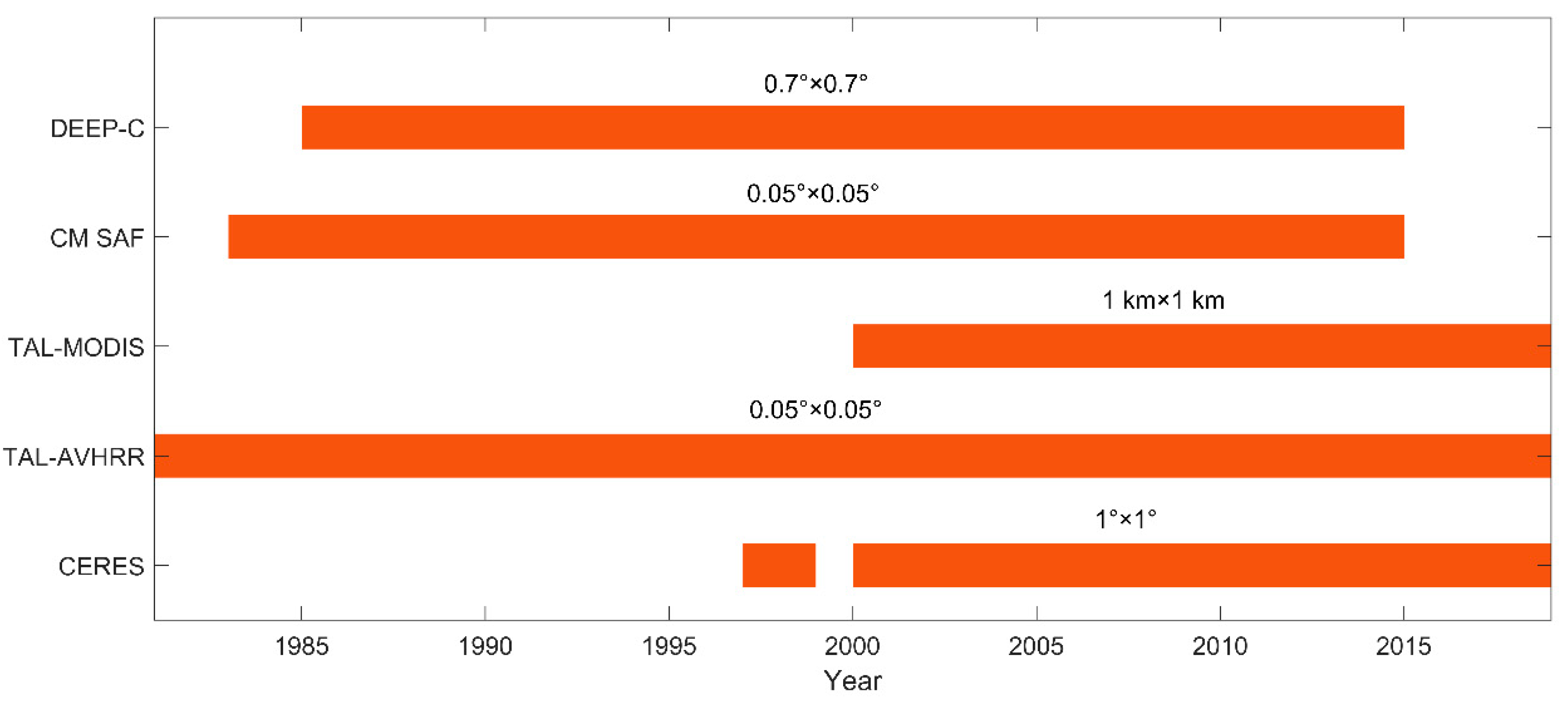
Figure 1 shows the time span of the five TOA albedo products assessed in this study. Each dataset is briefly described in the following section.
2.1. Clouds and the Earth’s Radiant Energy System (CERES)
CERES, a broadband instrument on board Terra, Aqua, and Suomi NPP, measures shortwave reflected radiation (0.3–5 μm), longwave thermal radiation (8–12 μm), and all wavelengths of radiation (0.3–200 μm) [
28]. The spatial resolution of CERES on Terra and Aqua is nearly 20 km at the nadir. Based on the observed shortwave radiance, the CERES shortwave fluxes have been developed using an angular distribution model (ADM) [
10]. Moreover, the Level-2 Single Scanner Footprint (SSF) that provides instantaneous TOA albedo at a resolution of 20 km and the Level-3 Synoptic products (SYN1deg) that provide hourly, 3-hourly, daily, and monthly mean TOA radiative fluxes have also been developed [
29]. In this study, the SYN1deg data, which began in March 2000 at a resolution of 1 degree, were used in the intercomparison.
2.2. TOA Albedo from AVHRR Data (TAL-AVHRR)
Recently, Song et al. [
17] released a long-term record of TOA albedo over land generated from AVHRR data, which provides the longest continuous record of global satellite observations since 1981. Direct estimation models were built to derive instantaneous TOA broadband albedo. Cloudy-sky, clear-sky, and snow-cover conditions were separately considered, and the training data for building the model were from real AVHRR observations and high-resolution TOA albedo datasets retrieved from MODIS data [
15]. The instantaneous albedo values were converted to daily and monthly mean values based on the diurnal curves from the CERES 3-hourly flux dataset. The dataset has covered global land at a spatial resolution of 0.05 degree since 1981. Notably, the product has some gaps in 1994 and 2000 because of the unavailability of the source AVHRR data. It is the first long-term high spatial resolution TOA albedo product with global coverage over land.
2.3. TOA Albedo from MODIS Data (TAL-MODIS)
Wang and Liang [
15] retrieved TOA albedo over land from multispectral data collected by MODIS using a hybrid method that is based on extensive atmospheric radiative transfer simulations considering various surface and atmospheric conditions. Different algorithms have been developed for clear-sky and cloudy-sky conditions, respectively. For the clear-sky condition, the Polarization and Directionality of the Earth’s Reflectances/Polarization and Anisotropy of Reflectances for Atmospheric Sciences coupled with observations from a Lidar (POLDER-3/PARASOL) bidirectional reflectance distribution function database has been used to consider surface reflectance anisotropy, thus generating TOA spectral and then broadband albedo. For the cloudy-sky condition, the surface is assumed to be Lambertian and the TOA broadband albedo is directly obtained. Similar to TAL-AVHRR, after generating the instantaneous TAL-MODIS, the daily/monthly mean TOA albedo is needed for further application. Instead of using the CERES 3-hourly flux dataset when generating daily TAL-AVHRR, the diurnal curves from the CERES hourly dataset were used to generate daily TAL-MODIS to improve the accuracy. The dataset has covered global land at a spatial resolution of 1 km since 2000. In this study, we aggregated it into a resolution of 0.05° for better intercomparison to other TOA albedo products.
2.4. Climate Monitoring Satellite Application Facility (CM SAF)
The CM SAF TOA Radiation Meteosat Visible and InfraRed Imager/Spinning Enhanced Visible and InfraRed Imager (MVIRI/SEVIRI) Data Record provides the TOA reflected solar and emitted thermal radiation under all sky conditions. The dataset covers a 32-year-time period from 1 February 1983 to 30 April 2015. The long data record is helpful in analyzing the changes in the Earth’s energy budget during the past several decades. Narrowband to broadband regressions have been derived based on the overlap between the MVIRI and Geostationary Earth Radiation Budget instruments from 2004 to 2006, and the CERES Tropical Rainfall Measurement Mission (TRMM) ADMs have been used to compute the TOA reflected solar radiation from the broadband radiances [
16]. The products include daily means, monthly means, and monthly averages of the hourly integrated values. The data covers the region 70°N–70°S and 70°W–70°E at a spatial resolution of 0.05°. It has the same resolution as that of TAL-AVHRR and its long-term series coverage also contributes to the intercomparison.
2.5. Diagnosing Earth’s Energy Pathways in the Climate System (DEEP-C)
The DEEP-C project reconstructed TOA radiative energy fluxes (outgoing longwave radiation (OLR), absorbed shortwave radiation (ASR), and net radiation) combining satellite data, atmospheric reanalysis (ERA-Interim), and climatic model (AMIP5) simulations [
30]. The TOA datasets cover the globe at a spatial resolution of approximately 0.7° from 1985 to 2015. CERES EBAF v2.8 data were used from March 2000 to May 2015. Therefore, a comparison with CERES over this period will only highlight differences in the EBAF version and spatial interpolation. From January 1985 to February 2000, the monthly mean radiative fluxes were reconstructed using monthly seasonal cycles from 2001–2005 CERES data, spatial distribution of radiative fluxes represented by ERAI data constrained by hemispheric mean changes in radiative fluxes from the Earth Radiation Budget Satellite (ERBS) wide field of view (WFOV) measurements. Note that DEEP-C only provides the ASR, which is calculated as the difference between incoming solar radiation from the Solar Radiation and Climate Experiment and CERES outgoing shortwave radiative flux, instead of the TOA albedo. Therefore, we calculated the TOA albedo with the TOA incoming solar flux from the CERES data.
2.6. Data Processing
As the five TOA albedo products were of different spatial resolutions, we compared them at three different spatial resolutions. TAL-AVHRR, TAL-MODIS, and CM SAF TOA albedo products at a 0.05° resolution were first compared, and then aggregated to 0.7° for comparison with DEEP-C, and finally were all aggregated to 1° to compare to the CERES TOA albedo product. The aggregation was weighted by the grid areas, which varied with latitude.
For CM SAF, the calculation is straightforward as it includes both the shortwave upward fluxes and the shortwave downward fluxes. For DEEP-C, however, as it only contains the TOA ASR, we needed to use the shortwave downward fluxes from other datasets. Considering that the CERES data are of relatively high accuracy and the TOA incoming solar flux is relatively constant, we calculated the mean value of the CERES TOA incoming solar flux for each month from 2001 to 2016. By subtracting the ASR from DEEP-C, the shortwave upward fluxes at TOA were obtained. Finally, the TOA albedo of the DEEP-C dataset was calculated.
The intercomparison was performed at different spatial extents including global, latitudinal, and regional scales. The latitudinal average was calculated for each 30° latitudinal band, and the regional average was calculated based on different regions. The comparison was also performed during different seasons: December–January–February (DJF), March–April–May (MAM), June–July–August (JJA), and September–October–November (SON), where the December value is from the previous year. Notably, TAL-AVHRR and TAL-MODIS include only land, while the other three products include both land and ocean. Therefore, before the intercomparison, we extracted the land from the other three products using a global land mask.
3. Results Analysis
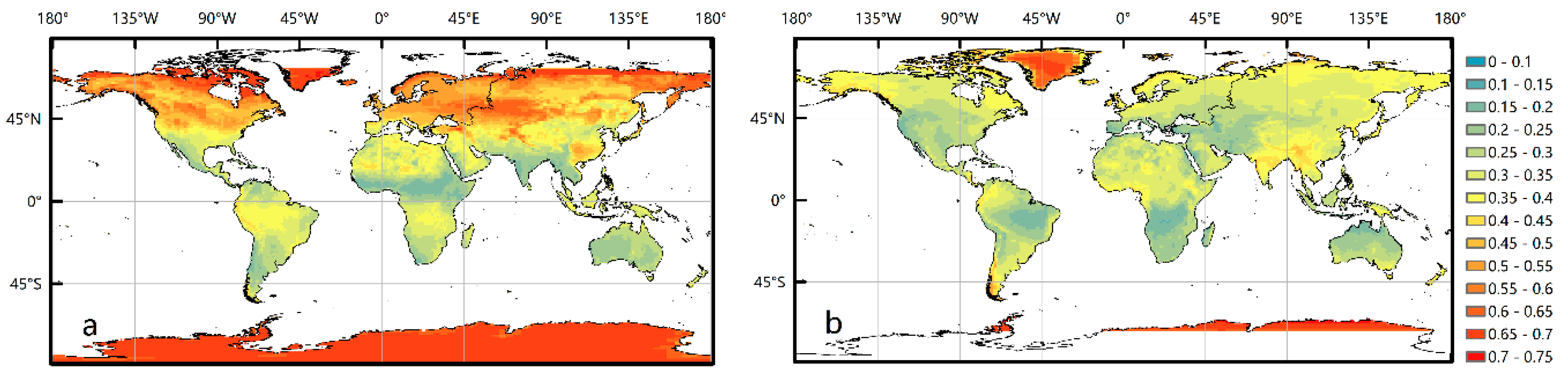
Figure 2 shows the average TOA albedo of CERES from 2001 to 2017 in January and July, respectively. From
Figure 2, one can see that Greenland and Antarctica stand out because of the high TOA albedo value due to the ice/snow cover, and the values in the northern hemisphere winter were also relatively larger. Next, five TOA albedo products were intercompared at three different spatial resolutions (0.05°, 0.7°, and 1°), respectively. Considering that percentage differences, which are obtained from dividing the difference of two products by their average, are more meaningful than absolute differences, all the difference maps shown in this study (
Figure 3,
Figure 4,
Figure 5 and
Figure 6) are presented and discussed in percentage differences.
3.1. Intercomparisons at 0.05° Spatial Resolution
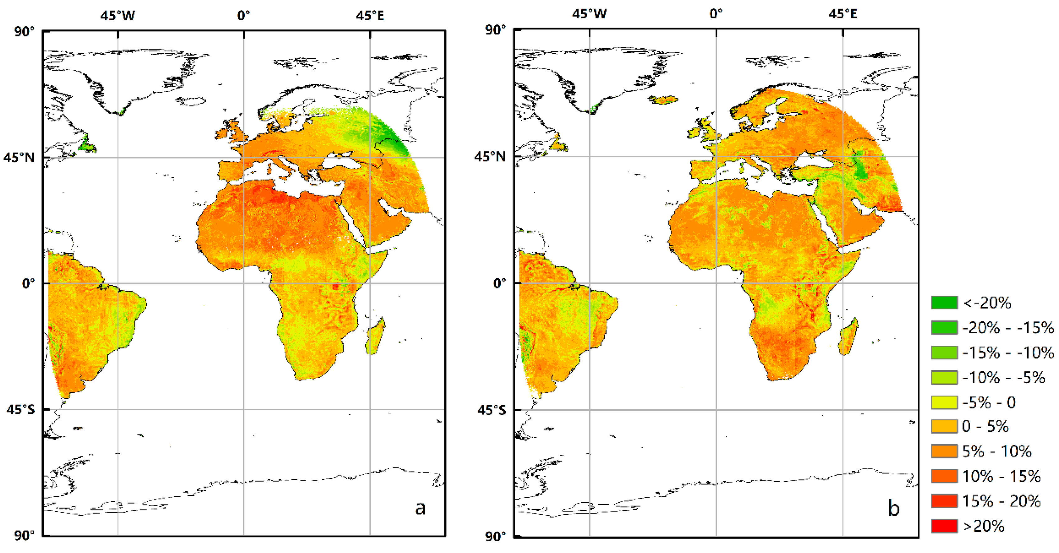
To determine the exact differences in distribution between CM SAF and TAL-AVHRR, we calculated the differences in the mean value of the TOA albedo from 1984 to 2014 using CM_SAF minus TAL-AVHRR with 1994 and 2000 excluded because TAL-AVHRR had some gaps due to the unavailability of the source AVHRR data in these two years.
Figure 3a shows that the percentage differences were mostly less than 20%, but much larger around 50°N, 50°E in January. As for July, most of the differences were positive, indicating that overall CM SAF was larger than TAL-AVHRR in July.
Figure 4 shows the differences in the mean value of the TOA albedo from 2001 to 2014 using TAL-MODIS minus TAL-AVHRR. From this figure, one can see that in January, the TOA albedo was lower in AVHRR than MODIS in most regions in the northern hemisphere while in July, the differences were quite large around 70°N.
3.2. Intercomparisons at a 0.7° Spatial Resolution
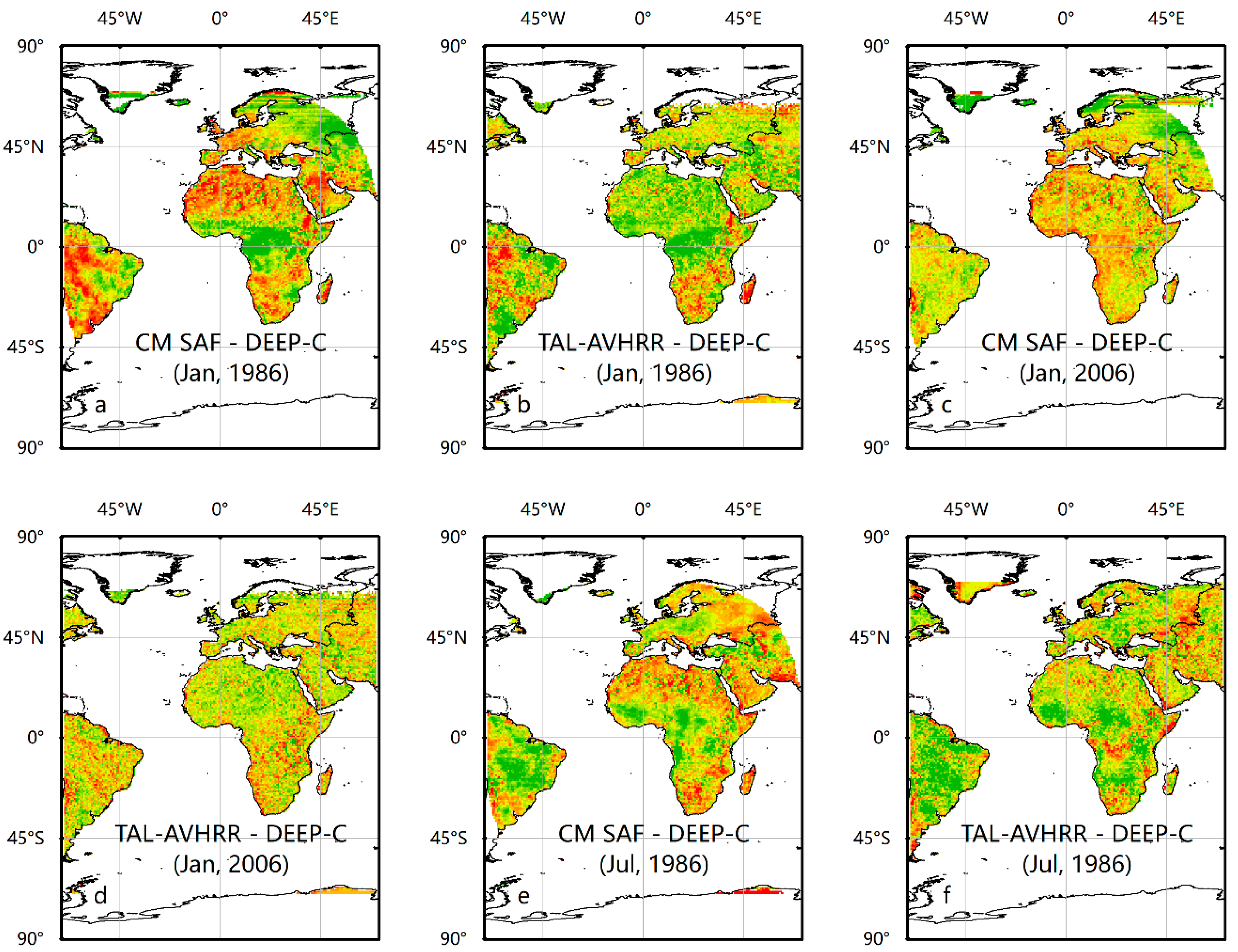
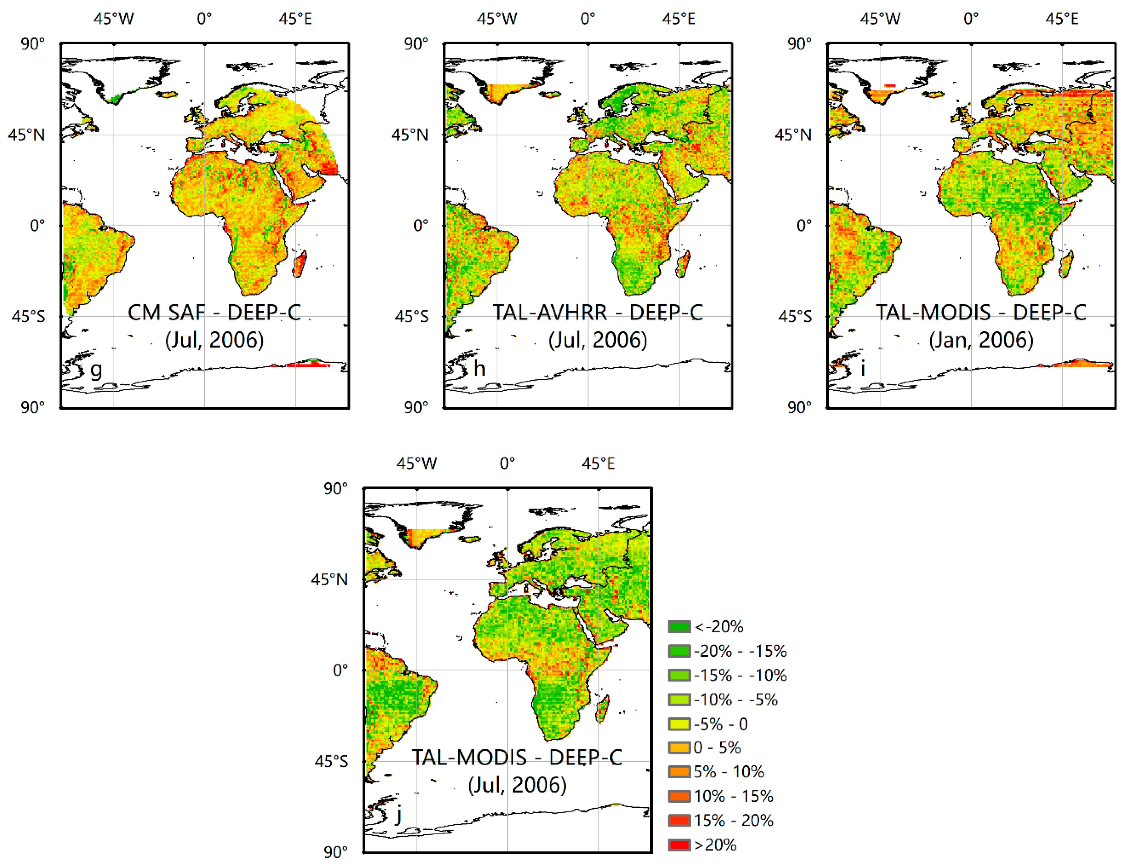
Four TOA albedo products (TAL-AVHRR, TAL-MODIS, DEEP-C, and CM SAF) were intercompared at a 0.7° spatial resolution. Considering that DEEP-C products are generated using different source data before and after 2000, we chose the year 1986 and 2006 for intercomparison. Additionally, as the spatial resolution of 0.7° and 1° are quite close, here we chose the area of 70°N–70°S and 70°W–70°E to show more detailed information. The results are shown in
Figure 5. Overall, the percentage differences between the four products were less than 20%. The differences between TAL-AVHRR and DEEP-C were relatively smaller than the differences between CM SAF and DEEP-C. In addition, the differences between these products become smaller after 2000.
3.3. Intercomparisons at a 1° Spatial Resolution
All five TOA albedo products, aggregated into a 1° × 1° spatial resolution, were intercompared, and the global and regional differences between these products are presented here.
3.3.1. Global Differences
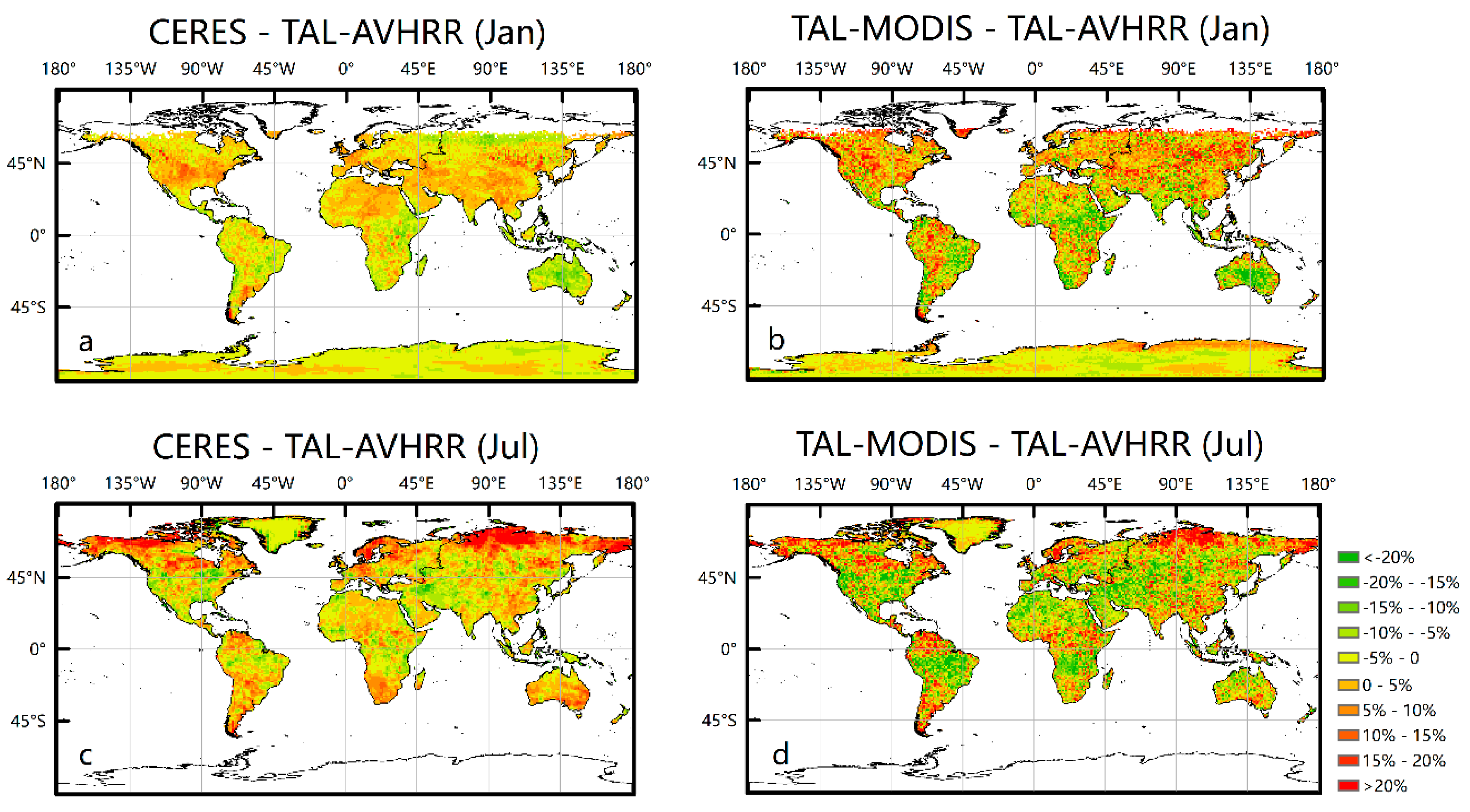
Figure 6a,b show differences in the mean value of the TOA albedo in January 2006 between CERES and TAL-AVHRR, and the differences between TAL-MODIS and TAL-AVHRR, respectively. Overall, the differences between CERES and TAL-AVHRR in January were the smallest out of the four. The distribution of the differences between TAL-MODIS and TAL-AVHRR in January was quite irregular. In July, the pattern of
Figure 6c,d was similar, and there were obvious differences in the high-latitude area, except for Greenland. However, most of the percentage differences were less than 20%.
It is not sufficient to conduct intercomparisons only at a global scale over land because these products may perform differently among different regions. To comprehensively compare these products, the regional differences need to be calculated and analyzed.
3.3.2. Regional Differences
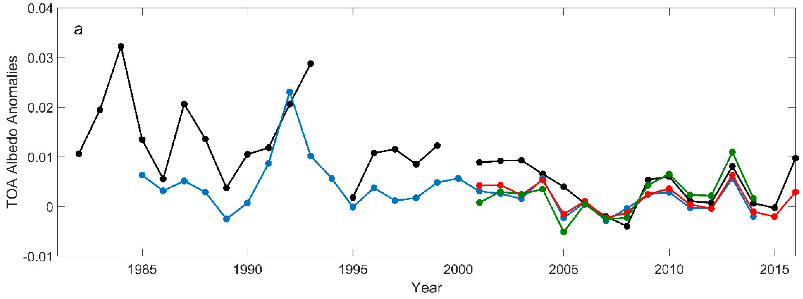
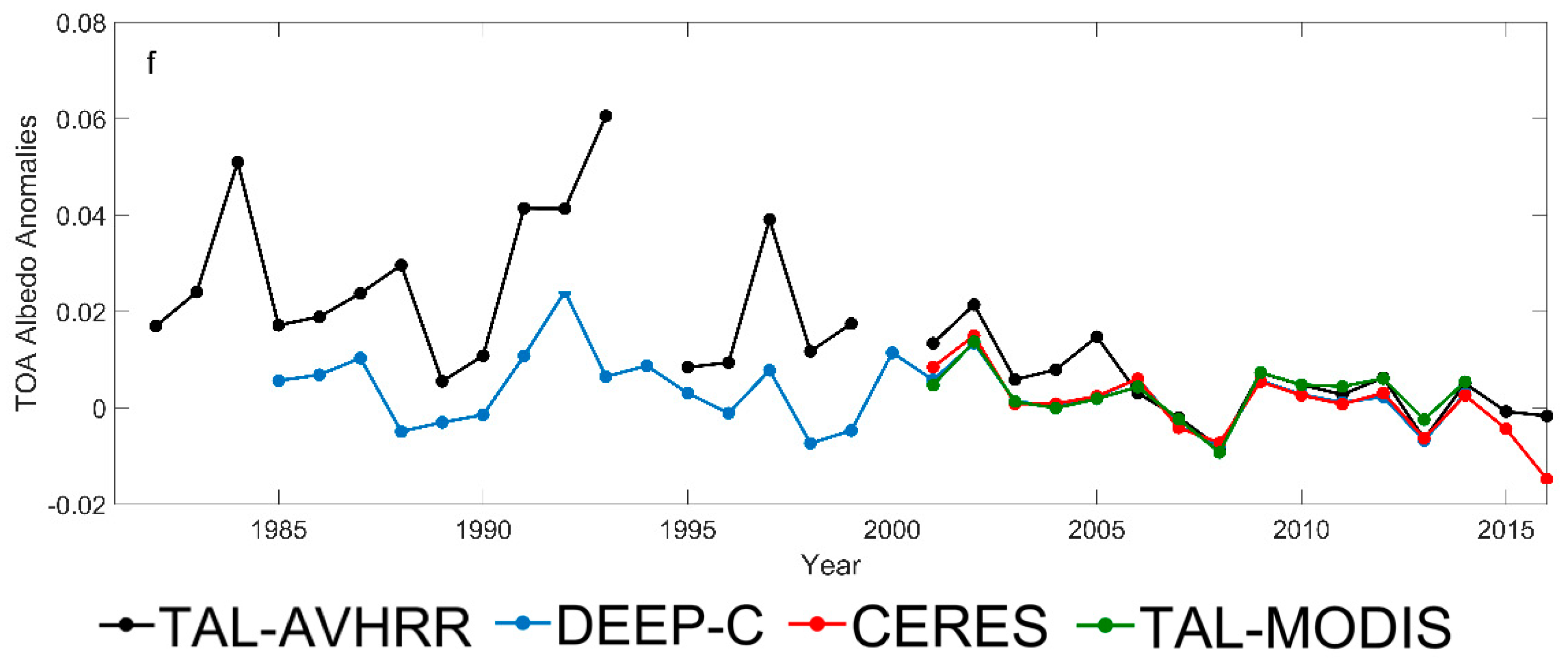
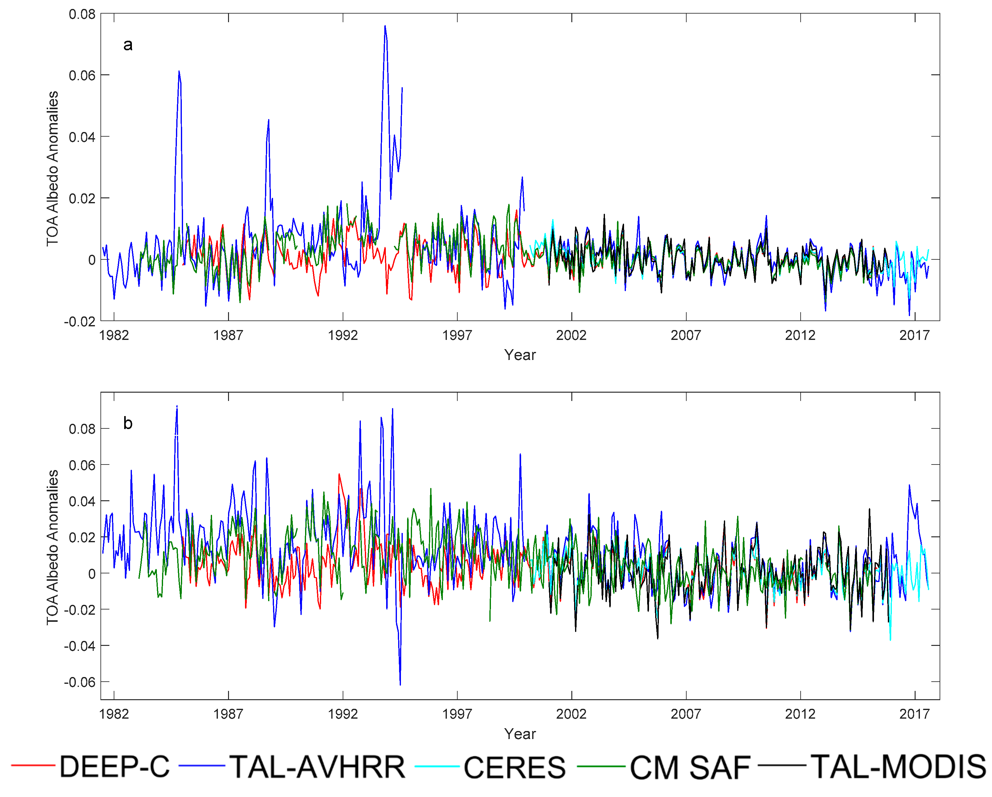
As
Figure 7 shows, the black, green, blue, and red lines stand for the TAL-AVHRR, TAL-MODIS, DEEP-C, and CERES monthly mean TOA albedo anomalies of different latitudinal bands, respectively. CM SAF was excluded in this part due to the limited spatial coverage. Before 2000, the differences between TAL-AVHRR and DEEP-C were much larger, and DEEP-C showed a more stable trend than that of TAL-AVHRR. Notably, there was an obvious peak value during 1992 in the Northern Hemisphere caused by the eruption of Mount Pinatubo in the Philippines in 1991. After 2000, when the CERES data and TAL-MODIS were included in the intercomparison, one can see that overall, DEEP-C matched very well with the CERES data. This is not surprising because CERES data were used after 2000 to develop the DEEP-C datasets. In addition, overall, TAL-MODIS matched well with the DEEP-C and CERES data. As AVHRR becomes much more stable after 2000, TAL-AVHRR matched much better with DEEP-C during this period. The largest difference between TAL-AVHRR and DEEP-C decreased from 0.05 before 2000 to 0.007 after.
To fully understand how different TOA albedo products perform in different regions, we divided the world area into ten parts, as shown in
Figure S1 [
31,
32]. The division overall matched that of Rao’s work [
31], except for some small changes in the boundary of Europe and Asia. Specifically, the boundary of Europe was set as 70°N instead of 80°N because of the limit of the coverage of CM SAF. The boundary of Asia1 was set as 60°E instead of 45°E to avoid overlap with the coverage of Europe. We made comprehensive intercomparisons among the five products by analyzing their performance in these ten regions, respectively.
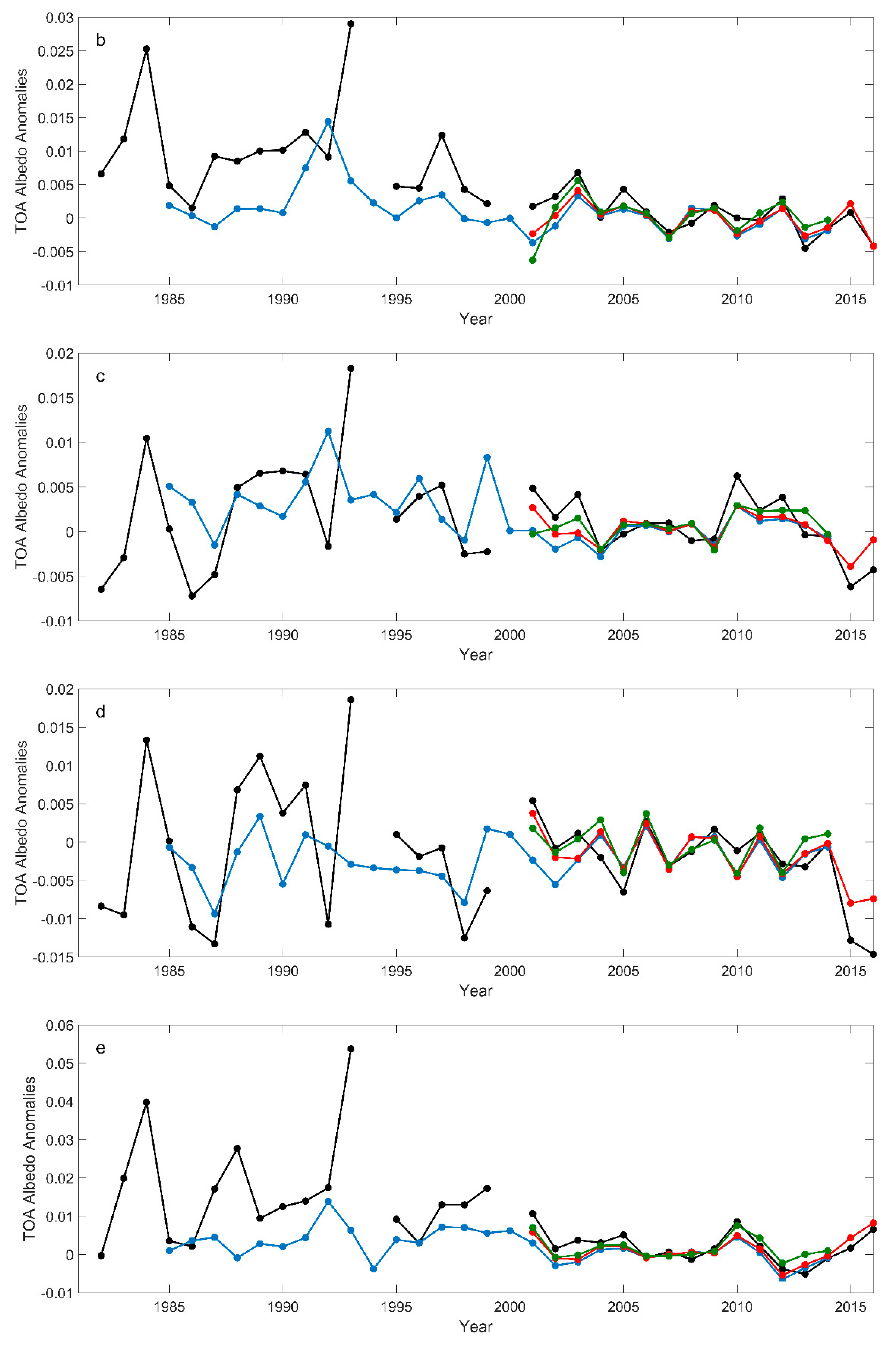
The monthly mean TOA albedo anomalies of Africa and Europe are shown in
Figure 8. The results were deseasonalized by subtracting the average values of each season when calculating the anomalies. Five products were compared in this region, and
Figure S2 shows the results of other regions. From these figures, one can see that the differences among TAL-AVHRR, DEEP-C, and CM SAF were much larger before 2000, particularly the differences between TAL-AVHRR and the other two products. Specifically, the differences between the anomalies of TAL-AVHRR and DEEP-C could be close to 0.08 during some years before 2000. The differences between DEEP-C and CM SAF in Europe and Africa, however, were much smaller.
As some overestimations and underestimations in these datasets are seasonally dependent and can be removed following the deseasonalizing process [
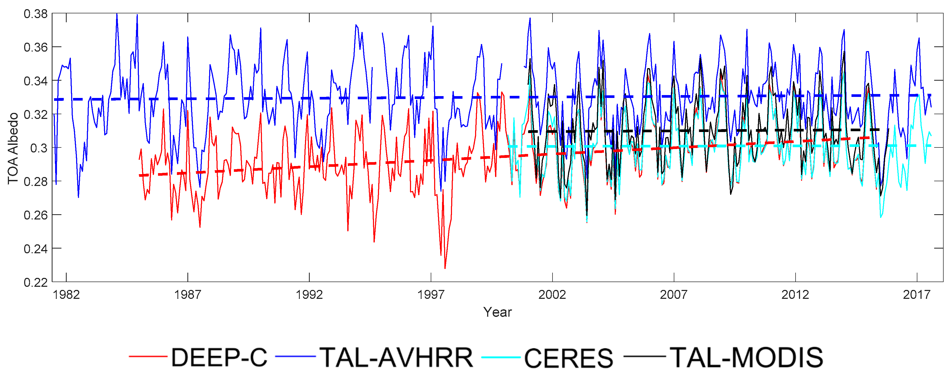
17], some differences may not be shown in this figure. Therefore, we also calculated the absolute value of the DEEP-C, TAL-AVHRR, TAL-MODIS, CERES, and CM SAF monthly mean TOA albedo for different regions.
Figure 9 indicates the results of the Maritime Continent (MCT). The results of the other regions are shown in
Figure S3.
After calculating the corresponding absolute values, we found that there were obvious overestimations in TAL-AVHRR, and that they were larger during the years before 2000, as shown in
Figure 9. This figure corresponds to the region of MCT, corresponding to the area of Indonesia, a country consisting of more than 17,000 islands. Considering that TAL-AVHRR only generates TOA albedo over land, islands may easily lead to overestimations as mixed pixels always occur in islands, particularly those that are small.
The root mean square differences (RMSD) and mean differences (MD) between different products during different periods are summarized in
Table 1 and
Table 2. The maximum RMSD and MD were 0.031 and 0.011, respectively, corresponding to the difference between TAL-AVHRR and DEEP-C during autumn in the region 90°N–90°S and 70°E–180°E. The RMSDs were smaller when comparing the difference between TAL-AVHRR and CERES with the difference between TAL-AVHRR and DEEP-C. By comparing
Table 1 to
Table 2, one can see that the RMSDs of CM SAF did not change much, while the RMSDs of TAL-AVHRR during all seasons became much smaller after 2000 and TAL-MODIS performed relatively well. In addition, as most of the MDs of TAL-AVHRR were positive values, one can conclude that there were more overestimations of TAL-AVHRR than underestimations among the different regions. In the regions 70°N–70°S and 70°W–70°E, the MD of TAL-AVHRR decreased because this region does not contain high-latitude areas, also indicating that TAL-AVHRR does not perform well in high-latitude regions.
4. Discussion
In this study, there was good consistency among the five TOA albedo products after 2000. This is partly because DEEP-C uses CERES data after 2000, which was mentioned in
Section 2.5. In addition, CERES data were also used when converting the instantaneous TAL-AVHRR and TAL-MODIS to the daily ones. However, considering that for these two datasets CERES data were only used to determine the conversion ratios, which are dependent on the observation time, the location, and the day of the year, it can be concluded that the good consistency between CERES, TAL-MODIS, and TAL-AVHRR shown in this study was not due to the usage of CERES data when generating the monthly TAL-MODIS and TAL-AVHRR, whose accuracy mostly depends on the accuracy of the retrieved instantaneous TOA albedo values.
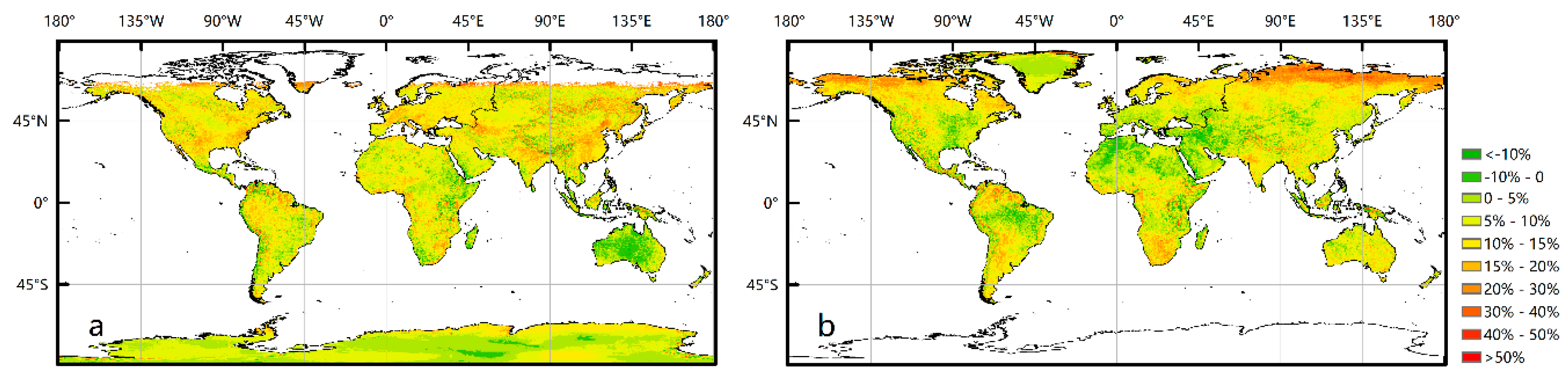
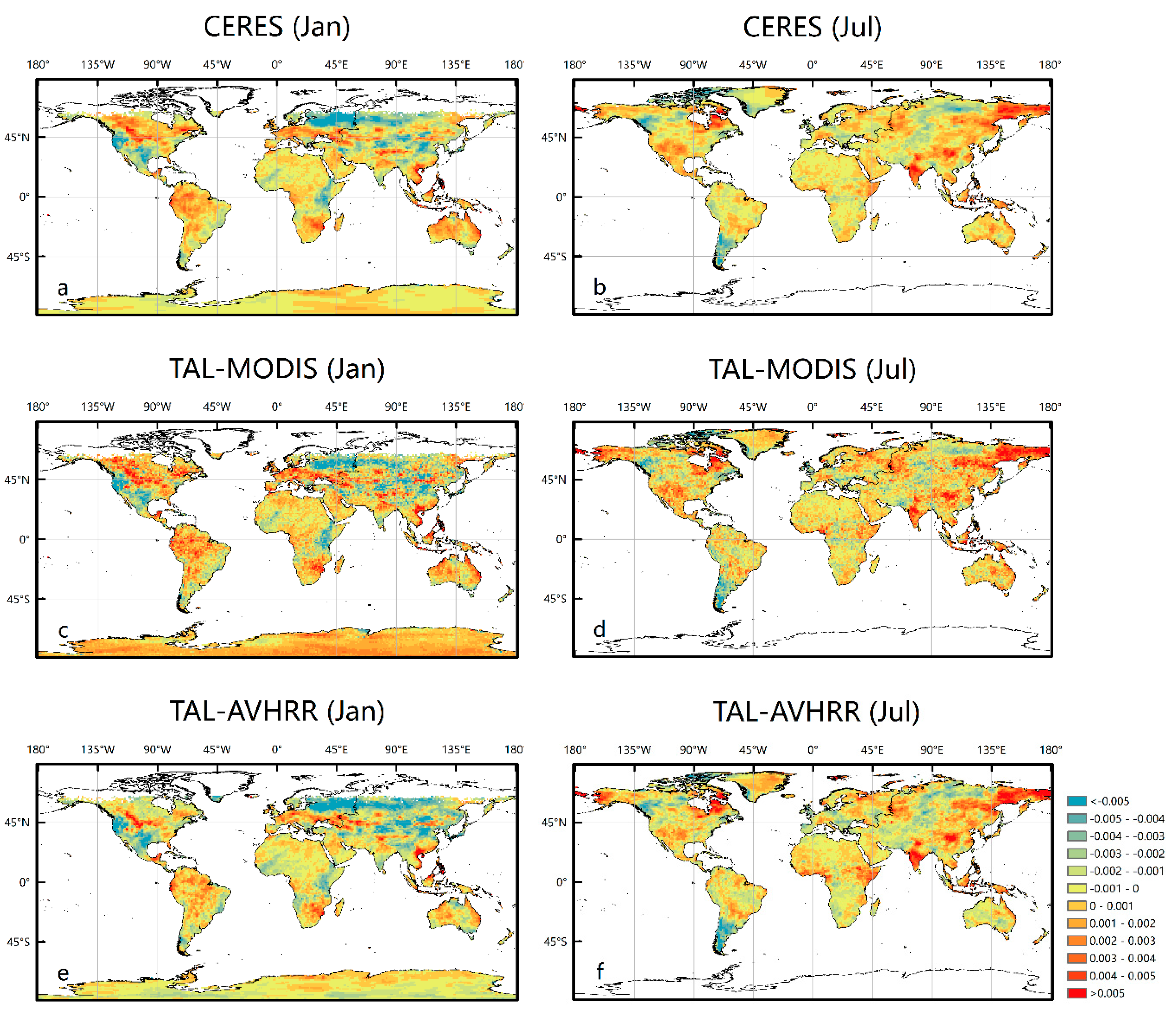
These three products were used to calculate the trends of the TOA albedo in a 1° × 1° grid based on the period 2001–2014 to show their differences in quantifying the variations at a global scale. The three products showed a similar pattern both in January and July, with an increase in the north of America, west of Europe, most parts of South America and Australia in January, and northeast of Asia in July, and a decrease in the east of Europe in January, and south of South America in July (
Figure 10). TAL-AVHRR demonstrated a smaller trend magnitude than CERES and TAL-MODIS in the north of America and Australia in January, while in July, the three products showed quite similar patterns. The trends of the TOA albedo in the Antarctica were quite different in January, especially between TAL-MODIS and the other two, while in July, the trends of CERES in a small part of Greenland were the opposite to the other two. Specifically, CERES showed a decreasing trend (−0.001 year
−1) in the west part of Greenland, while the other two showed an increasing trend (0.001 year
−1). However, the trend was quite close in the east part of Greenland (0.001 year
−1). Therefore, users should be careful when calculating the trend of the TOA albedo to prevent inconsistent conclusions, especially for high-latitude regions.
5. Conclusions
We examined the differences in five TOA albedo datasets (i.e., TAL-AVHRR, TAL-MODIS, CERES, DEEP-C, and CM SAF) over land at different spatial scales in this study.
By comparing four products (i.e., TAL-AVHRR, TAL-MODIS, CERES, and DEEP-C) at global scale, of which DEEP-C uses CERES data from the year 2000 onwards, we found that the four products matched well with each other overall in mid-low latitude regions, where the percentage differences were less than 20%. However, in some regions, particularly high-latitude regions, the differences were much larger. In addition to the problem of TAL-AVHRR during 1993 and 1994 caused by the unavailability of the source AVHRR data, TAL-AVHRR performed differently before and after 2000. Regarding the trend of the TOA albedo, CERES, TAL-MODIS, and TAL-AVHRR performed similarly, but significant differences were found in the high-latitude regions, especially for Antarctica in January.
To demonstrate how these five TOA albedo products performed regionally, we divided the world area into ten parts, and calculated the corresponding deseasonalized anomalies and the absolute values of the TOA albedo. The results showed that the deseasonalized anomalies of the five products matched relatively well with each other. Before 2000, the differences among the three products (i.e., TAL-AVHRR, DEEP-C, and CM SAF) were much larger, particularly the differences between TAL-AVHRR and the other two products. The differences between the TAL-AVHRR and DEEP-C anomalies could approach 0.1 during some years before 2000, while the differences between DEEP-C and CM SAF in Europe and Africa were much smaller.
TOA albedo products were widely used in climate dynamic studies as TOA albedo is the key component of the Earth’s energy budget. If the quality of the TOA albedo datasets is poor, inaccurate conclusions regarding the climatic system may be drawn, as a small underestimation or overestimation of the TOA albedo can lead to large errors when calculating the TOA shortwave upward flux. For the years before 2000, CM SAF is recommended for use in the mid-low latitude region of Africa and Europe, while DEEP-C is recommended in other regions. For the years after 2000, CERES and DEEP-C are recommended for use in the mid-low latitude regions while all five products are recommended for use in other regions.


