Estimating Penetration-Related X-Band InSAR Elevation Bias: A Study over the Greenland Ice Sheet

Abstract

Accelerating melt on the Greenland ice sheet leads to dramatic changes at a global scale. Especially in the last decades, not only the monitoring, but also the quantification of these changes has gained considerably in importance. In this context, Interferometric Synthetic Aperture Radar (InSAR) systems complement existing data sources by their capability to acquire 3D information at high spatial resolution over large areas independent of weather conditions and illumination. However, penetration of the SAR signals into the snow and ice surface leads to a bias in measured height, which has to be corrected to obtain accurate elevation data. Therefore, this study purposes an easy transferable pixel-based approach for X-band penetration-related elevation bias estimation based on single-pass interferometric coherence and backscatter intensity which was performed at two test sites on the Northern Greenland ice sheet. In particular, the penetration bias was estimated using a multiple linear regression model based on TanDEM-X InSAR data and IceBridge laser-altimeter measurements to correct TanDEM-X Digital Elevation Model (DEM) scenes. Validation efforts yielded good agreement between observations and estimations with a coefficient of determination of R² = 68% and an RMSE of 0.68 m. Furthermore, the study demonstrates the benefits of X-band penetration bias estimation within the application context of ice sheet elevation change detection.

1. Introduction

1.1. Motivation

In July 2012, satellite observations detected an extreme melt event covering 98.6% of the entire Greenland ice sheet [1,2]. Such remarkable events, which confirm the dramatic changes of the cryosphere, occur very rarely and have been observed only twice since the Medieval Warm Period [3]. Especially in the last two decades, a trend of accelerating melt of the Greenland ice sheet with increasing melt extent as well as lengthened melt season is emerging [1,3,4]. According to Shepherd et al. [5], the annual ice loss of the Greenland ice sheet was twice the annual loss compared to Antarctica in the period from 1992 to 2011 and has increased steadily. As stated by Flowers et al. and Van den Broeke et al. [6,7], a complete melting of the entire Greenland ice sheet would contribute to a global sea level rise of about 7 m, which will threaten hundreds of millions of people across the world [3]. Besides sea level rise, those changes in the cryosphere also play a major role in the Earth’s climate system with respect to the surface energy budget, the water cycle, primary productivity, and surface gas exchange [3]. Foremost, these changes will severely impact human livelihoods worldwide by means of an increased potential of flooding in coastal zones, consequences for agri- and aquaculture, marine shipping, oil and natural gas production, and tourism [3].

To face these concerning trends and associated challenges for the environment as well as human society, the changes in the cryosphere and their associated drivers must be identified and quantified. In this regard, remote sensing techniques offer the possibility to acquire up-to-date, reliable, and detailed information about the state and especially the dynamics of the cryosphere and thus facilitate our understanding and enable the development of sufficient adaptation and mitigation strategies. Interferometric Synthetic Aperture Radar (InSAR) systems in particular are well suited for the assessment of glaciers and ice sheets, since they provide 3D information with high spatial resolution over large areas without limitations due to weather conditions or illumination [8]. The dynamics of the global ice sheets (i.e., changing ice flow velocity and topography) are of highest interest in the context of the climate change [9,10,11] and can be estimated using multi-temporal InSAR-based elevation data. The German TanDEM-X (TerraSAR-X add-on for Digital Elevation Measurement) mission was the first single-pass SAR interferometer in space and enables highly accurate InSAR acquisitions without accuracy limitations caused by repeat-pass interferometry [12]. The objective of the TanDEM-X mission is the generation of a consistent, high-precision global Digital Elevation Model (DEM). According to Rizzoli et al. [13], the global TanDEM-X DEM provides high absolute height accuracy (i.e., overall absolute height accuracy of 3.5 m and absolute linear error of 90%); however, over highly vegetated and snow-/ice-covered regions, the height accuracy mainly suffers from volume decorrelation effects. Volume decorrelation over snow- and ice-covered regions is caused by penetration of the SAR signal into the snow pack [14]. Depending on the characteristics of the snow pack (e.g., snow density, grain size, and dielectric properties), different scattering and thus different penetration of the SAR signal occurs [15]. For estimation of the penetration bias, several approaches and techniques are proposed in the literature, which can be divided into two major categories.

Model-based approaches quantify the penetration bias by aiming to capture the underlying scattering mechanisms in order to estimate volume decorrelation and thus penetration of the SAR signal. For example, Hoen and Zebker [16] used correlation images of C-band ERS data for modeling penetration depth over Greenland. Dall [17] employed coherence for correction of the penetration-induced elevation bias in InSAR data by means of the coherent backscatter model. Oveisgharan and Zebker [18] modeled InSAR penetration based on a combination of radar brightness and correlation in the dry snow zone of Greenland. In addition, the model-based approach for estimation of penetration bias was transferred to polarimetric InSAR data by Stebler et al. and Fischer et al. [19,20].

In contrast, there are approaches that estimate the penetration bias based on empirically determined glacier facies. The glacier facies reflect the radar scattering characteristics of the snow pack and thus can be used to approximate InSAR penetration bias. These zones were related to ERS-1 SAR imagery over Greenland for the first time by Fahnestock et al. [21], who distinguished distinct backscatter signatures for the dry snow zone, the percolation zone, the wet snow zone, and the bare ice zone. In this regard, several studies investigated the delineation and classification of glacier facies over Greenland based on InSAR data (e.g., [8,22,23]). Most recently, Rizzoli et al. [24] employed fuzzy clustering of a mosaic of TanDEM-X radar backscatter over Greenland for classification of these four zones and estimated penetration bias assuming uniform snow density for each zone.

To evaluate X-band InSAR data for the investigation of glacial meltdown, the current study aimed to develop a generic and easily transferable pixel-based approach using the relationship between TanDEM-X penetration bias and interferometric coherence as well as backscatter intensity. In contrast to earlier studies, the proposed method works independently of prior knowledge on the physical properties of the snow pack (e.g., snow density, stratigraphy, and grain size) or the determination of the presence and number of glacier facies and thus enables the estimation of penetration-related elevation bias only on the basis of InSAR data. In detail, the aims of this study were defined as: (i) estimation of TanDEM-X penetration bias using a multiple linear regression model based on interferometric coherence and backscatter intensity; and (ii) application of the proposed approach to correct TanDEM-X DEM scenes and derive elevation change at a test site in the north of the Greenland ice sheet. In addition, the transferability of the proposed approach to the entire Greenland ice sheet based on multi-annual TanDEM-X InSAR data is discussed.

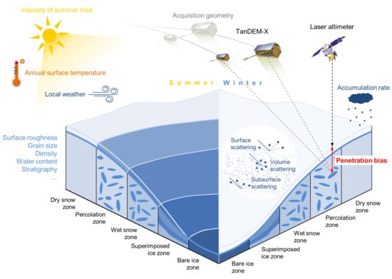
1.2. Conceptual Framework

As stated by Dall [17], InSAR elevation bias results from penetration of the radar signals into a volume. The penetration bias is defined as the difference between InSAR height (i.e., height of the phase center corresponding to the mean locus of backscatter) and the Earth’s surface elevation [16]. The penetration of the SAR signal is dependent on radar frequency, radar imaging conditions, and the physical and dielectric characteristics of the snow/ice layer [8].

In this study, TanDEM-X penetration bias $\Delta h$ is defined as the difference between TanDEM-X DEM $h_{TanDEM-X}$ and laser-altimeter surface height measurements of IceBridge $h_{IceBridge}$ and ICESat mission $h_{ICESat}$, respectively.

$$\Delta h=h_{TanDEM-X}- h_{IceBridge}$$

and

$$\Delta h=h_{TanDEM-X}- h_{ICESat}$$

Figure 1 illustrates the concept of InSAR penetration bias and its influencing factors. The physical properties of the snow pack, such as surface roughness, grain size, density, water content, and stratigraphy, determine the penetration of the SAR signal [25]. The snow and ice characteristics are in turn determined by snow metamorphism and ablation processes driven by accumulation, annual temperature variation, and summer melt, which vary with geographical location, surface elevation, and regional climate [26]. According to the snow morphology, distinct zones at the surface area of a glacier or an ice sheet (i.e., glacier facies) can be distinguished. For the Greenland ice sheet, five different zones (i.e., bare ice zone, superimposed ice zone, wet snow zone, percolation zone, and dry snow zone) were described initially by Benson [27]. Surface scattering, volume scattering, and subsurface scattering occur depending on the physical snow parameters and thus yield distinct backscatter signatures and signal penetration for each zone varying from season to season and from year to year. Besides, the scattering behavior of the SAR signals is influenced by the acquisition geometry (e.g., effective baseline of the InSAR system, incidence angle, and look direction). The different interaction of the SAR signals with the surface of the glacier in each zone results in different InSAR penetration bias with local variations. Interferometric coherence, defined as the normalized cross-correlation of the two SAR images, and backscatter intensity are strongly related to the glacier zones and thus to InSAR penetration bias [18,28,29].

The bare ice zone is characterized by varying surface roughness and dynamic structures such as crevasses and cracks [21]. During winter, the ice is covered by dry snow, which will have melted by the end of the ablation period [30]. In general, the bare ice zone is dominated by surface scattering with low interferometric coherence and backscatter intensity, which decreases during summer due to the presence of meltwater. Penetration of the SAR signals is very low underlying seasonal variations [16], which causes only small penetration bias.

The superimposed ice zone results from refreezing of meltwater [21]. At the end of summer, the snow cover from winter has completely melted and the meltwater forms a new layer of superimposed ice on the cold glacier surface dependent of the local topography. During the refreezing process, small air bubbles (with a size ranging from mm to cm) are trapped in the new ice layer, depending on the time of refreezing [31]. In winter, backscatter intensity is low due to volume scattering caused by the air bubbles, whereas it is very low in summer due to surface melt. In years with pronounced ablation, this zone may not exist, whereas, in years of reduced ablation, the superimposed ice zone may be separable from the bare ice zone based on its higher degree of smoothness [30]. The superimposed ice zone is characterized by small penetration bias due to weak signal penetration varying with season.

The snow in the wet snow (i.e., soaked snow) zone reaches the melting point as a result of latent heat released by extensive refreezing of meltwater [21], yielding recrystallization and larger grain sizes. The entire annual accumulation of snow is subject to melting and refreezing, which results in the formation of ice inclusions (i.e., ice lenses, pipes, and layers) [30]. Higher interferometric coherence and backscatter intensity than in the superimposed ice zone are caused by ice inclusions, which become less effective scatterers in summer due the saturated snow [32]. Greater penetration bias compared to the bare and superimposed ice zone can be observed.

In the percolation zone, surface snow is subject to melt and percolates down through the cold firn forming massive layers and vertical as well as horizontal oriented pipes of solid ice by refreezing [32]. According to Benson [27], the transition from the wet snow zone to the percolation zone on the Greenland ice sheet takes places over a few kilometers only. The ice inclusions can have dimensions that are comparable or larger in relation to the wavelength of the X-band SAR and act as dihedral or dipole scatterers in the subsurface inducing strong backscatter and high interferometric coherence in winter [21,32]. In contrast, surface melt leads to dominant surface scattering with low backscatter intensity and interferometric coherence in summer. Smaller penetration bias than in the wet snow zone can be observed depending on the vertical position of the ice inclusions, which is subject to seasonal variations.

In the dry snow zone at higher altitudes, the snow is gradually compacted under its own weight or metamorphosed under the effect of wind or depth-hoar development [30]. The transition from the percolation zone to the dry snow zone gradually takes place over a greater distance, inducing a smooth transition to low interferometric coherence and backscatter intensity. The absence of ice inclusions as well as small grain size increase volume scattering [16] and cause a significant loss of coherence due to deeper signal penetration (i.e., greater penetration bias) and reduced backscatter intensity.

All zones are subject to small-scale variations. In general, interferometric coherence and backscatter intensity reflect the properties of the glacier surface, which are directly related to InSAR penetration bias. Therefore, interferometric coherence and backscatter intensity are relevant for estimating the InSAR penetration bias.

2. Study Area

The Greenland ice sheet is the Earth’s second largest continuous ice body after the Antarctic ice sheet. It covers about 1.7 million km² (i.e., about 80% of Greenland’s land surface), which equals approximately five times the territory of Germany, with a volume of about 2.8 million km³ [33]. The geographical position of the ice sheet ranges from 59° to 83° north (i.e., about 2600 km) and from 73° to 110° west (i.e., 1200 km) [33]. The ice thickness is on average 1.6 km and more than 3 km at its thickest point [34]. Greenland is characterized by polar and subpolar climate with average temperatures below ten degrees in summer [35].

The study area is located in the north of the Greenland ice sheet (Figure 2). Each of the two test sites covers TanDEM-X data takes acquired from south to north in ascending orbit direction. Along this path, the land cover changes from dry snow zone at the most southern point of each test site across all glacier zones to rocks at the coast. In the following, the two test sites are referred to as the western and eastern site, respectively. TanDEM-X data corresponding to the red footprints in Figure 2 were used for model calibration and validation while TanDEM-X data corresponding to the blue footprints were used to further validate and verify the transferability of the model.

3. Datasets

3.1. TanDEM-X Elevation Data

The TanDEM-X mission provides interferometric X-band (9.65 GHz) data and enables the generation of a worldwide, consistent DEM with a globally unpreceded spatial resolution of 0.4 arc seconds (i.e., about 12 m) [12]. The mission is composed of the two almost identical satellites TerraSAR-X (launched in 2007) and TanDEM-X (launched in 2010) flying in a closely controlled formation. The simultaneous acquisition avoids possible errors due to temporal decorrelation and atmospheric disturbances [36]. Single-polarized (HH) interferometric TanDEM-X image pairs acquired in bistatic StripMap mode were used to generate digital elevation models for each single scene which were combined to the global TanDEM-X DEM [37].

For generation of single-scene DEMs, so-called RawDEMs, the backscattered signals are combined to an interferogram and the resulting phase differences are converted into height based on the interferometer geometry. The processing chain including data take analysis, common parameter calculation, synchronization, bistatic focusing, filtering, co-registration, phase unwrapping, and geocoding is implemented within the Integrated TanDEM-X Processor (ITP) [38,39]. The geocoded elevation information of the DEM scenes reflects the location of the mean phase center resulting from single or multiple backscattered signals within the same resolution cell and thus is dependent on signal penetration [13].

The global TanDEM-X DEM over Greenland is based on a mosaic of acquisitions from winters 2010/2011 (first coverage) and 2011/2012 (second coverage), as well as additional third and fourth coverages for steep coastal areas, which were acquired until mid-2014. Previously, all DEM scenes were calibrated to the rocky coast by the use of ICESat laser-altimeter measurements [40,41].

In this study, TanDEM-X InSAR data takes from winter 2010/2011 and winter 2011/2012 were used (

Table 1. TanDEM-X InSAR data takes used in this study. The value ranges of the incidence angle and the effective baseline are defined by the minimum and maximum value corresponding to the acquisition time.

Acquisition Date	Number of Scenes	Polarization	Orbit	Look Direction	Incidence Angle	Effective Baseline
5 April 2011	8	HH	Ascending	Right	40.6–40.6°	101.9–109.2 m
2 April 2012	8	HH	Ascending	Right	41.4–41.5°	178.2–189.2 m
10 April 2012	8	HH	Ascending	Right	39.4–39.5°	170.3–182.0 m

). As depicted in Figure 2, two TanDEM-X data takes from April 2012 were used for model calibration and validation (red TanDEM-X footprints) and one data take acquired in April 2011 was used to further validate and verify the transferability of the derived model as well as investigate the impact of penetration bias on elevation change detection (blue TanDEM-X footprints). The DEM, interferometric coherence (COH) and amplitude (AMP) are used.

3.2. ICESat Data

The ICESat (Ice, Cloud and land Elevation Satellite) mission operated from February 2003 to October 2009 and provided global spaceborne laser-altimeter data with a spatial resolution of 60–70 m and a sampling distance of 170 m along-track and 80 km across-track, respectively. The primary aim of the ICESat mission was to measure ice sheet mass balance, cloud, and aerosol heights, as well as land topography and vegetation characteristics [42]. In accordance with Rizzoli et al. and Wessel et al. [24,41], the ICESat GLA 14 product (Global Land Surface Altimetry Data) [42] was used as surface reference height for empiric approximation of the TanDEM-X penetration bias at large spatial scale (i.e., the entire Greenland ice sheet) in this study.

3.3. IceBridge Data

Due to the temporal inconsistency of ICESat elevation data and TanDEM-X DEM data takes, additional IceBridge data were employed in this study. IceBridge is an airborne mission that is repeated annually over the Arctic, Greenland, and Antarctica to bridge the temporal gap between the cessation of data collection by ICESat in 2009 and the launch of the ICESat-2 satellite on 15 September 2018. The IceBridge mission offers elevation measurements based on the same laser-altimeter as ICESat with an increased spatial resolution with a footprint size of 1–3 m and varying sampling distance [43]. For determination of reference values of the TanDEM-X penetration bias, IceBridge ATM L2 Icessn Elevation data [44] were used. The model calibration and validation were based on IceBridge laser-altimeter measurements acquired during the period from 30 March 2012 to 16 May 2012 and the transfer and application of the model were based on IceBridge laser-altimeter measurements acquired on 29 March 2011. The dataset contains resampled and smoothed elevation measurements of Greenland ice sheet surface acquired using the NASA Airborne Topographic Mapper (ATM) instrumentation [44].

4. Methods

A multiple linear regression model based on interferometric coherence and backscatter intensity was used to estimate X-band penetration bias. Figure 3 depicts the workflow of the current study. In a first step, the TanDEM-X data were pre-processed including preparation and adjustment of interferometric coherence, radiometric calibration of backscatter intensity, and calibration of the DEM. In a second step, the TanDEM-X data acquired in 2012 and the IceBridge laser-altimeter measurements were combined and used to fit the regression coefficients of the multiple linear model and to validate the accuracy. Finally, the derived model was applied to all TanDEM-X datasets in order to estimate the penetration bias. Subsequently, the calibrated DEM scenes from 5 April 2011 and 2 April 2012 were corrected and elevation change was derived.

4.1. Pre-Processing

4.1.1. Preparation and Adjustment of Interferometric Coherence

The interferometric coherence is influenced by the acquisition geometry as well as the properties of the scatterer [45]. As only the properties of the snow pack are to be detected, the impact of acquisition geometry must be mitigated for datasets with deviating effective baseline. Analyzing the relationship between penetration bias and interferometric coherence for the data used in this study (with quite large baselines differences of about 80 m) revealed a change in this relationship depending on the effective baseline between the two satellites. Figure 4a) shows the relationship of penetration bias based on ICESat and IceBridge (if available) and interferometric coherence averaged per individual DEM scene, while Figure 4b illustrates the used datasets. The spatial separation of the two antennas cause different illumination angles for the two images and thus different backscatter at the ground [16]. The difference between the two images will be small for short baselines, but will increase with baseline length until the critical baseline is reached and the two images are completely decorrelated [45]. This systematic loss in interferometric coherence is enhanced with increasing volume scattering (i.e., deeper signal penetration into the snowpack). According to Figure 4, it can be assumed that longer baselines decrease coherence, but do not influence the penetration bias.

To correct this effect on the dataset comprising TanDEM-X acquisitions with significantly deviating effective baselines, the interferometric coherence data from 2011 were adjusted to the data from 2012. Therefore, the trend of the coherence depending on signal penetration was calculated. The coherence values corresponding to the April 2011 acquisitions were projected onto the regression line corresponding to the effective baselines of the April 2012 acquisitions (Figure 4) according to:

$$CO{H}_{2011}{}_{corr}=\frac{-22.92-\left(-14.78\right)}{16.57}+\frac{24.45}{16.57}·CO{H}_{2011}$$

4.1.2. Radiometric Calibration of Backscatter Intensity

Several studies prove the capability of the backscatter coefficient ${\sigma }^0$ (i.e., backscatter level projected onto the ground [46]) for the retrieval of snow and ice characteristics (e.g., [28,30,47]). As stated by Ashcraft et al. [47], ${\sigma }^0$ is sensitive to snow grain size, wetness, and subsurface features and is therefore suitable for mapping of glacier facies and their variations. Thus, ${\sigma }^0$ was used in this study to employ the relationship between backscatter intensity and TanDEM-X penetration bias. ${\sigma }^0$ is derived from each single amplitude scene [48] according to

$${\sigma }^0=(k_s·{\left|AMP\right|}^2-NEBN)·\sin {\theta }_{loc},$$

and converted to Decibel

$${\sigma }^0{}_{dB}=10·{\log }_{10}{\sigma }^0,$$

where AMP is the backscatter intensity in digital numbers (pixel intensity value); $k_s$ is the calibration and processor scaling factor for the SAR signals annotated in the supplied metadata [49]; $NEBN$ is the Noise Equivalent Beta Nought, which represents the influence of different noise contributions to the signal and is annotated in the supplied metadata in form of polynomials over range with azimuth time tags describing the noise power; and ${\theta }_{loc}$ is the local incidence angle [48,50].

4.1.3. Height Calibration

To correct remaining systematic height errors after phase unwrapping and geocoding within the ITP, an offset from the operational TanDEM-X DEM Calibration and Mosaicking Processor [49] was applied. As opposed to the calibration of the global TanDEM-X DEM [40], two time-staggered TanDEM-X DEM mosaics were created for data acquired in 2011 and 2012, respectively [51]. Calibration offsets between −0.8 and 0.4 m were determined for the investigated data takes. This absolute height calibration is an important step as it ensures the derivation of comparable elevation values between different data takes.

4.2. Estimation of X-Band Penetration Bias

The penetration bias $\Delta h$ was estimated using a multiple linear regression model based on the interferometric coherence COH and the backscatter coefficient ${\sigma }^0{}_{dB}$.

$$\Delta h= a_0+a_1·COH+ a_2·{\sigma }^0{}_{dB},$$

where $a_0$, $a_1$, and $a_2$ are the regression coefficients. The penetration bias was estimated by the calculated regression plane of the linear model, deriving the expected value of $\Delta h$ for specific values of $COH$ and ${\sigma }^0{}_{dB}$. The regression plane describes the best fit among penetration bias, interferometric coherence, and backscatter intensity with $a_0$ as the intercept. To fit the model, the difference between TanDEM-X DEM and IceBridge elevation measurements, mean interferometric coherence, and mean backscatter intensity at each IceBridge footprint were used as $\Delta h$, $COH$, and ${\sigma }^0{}_{dB}$, respectively. The dataset comprising 87,097 data samples was based on TanDEM-X acquisitions from 2 April 2012 and 10 April 2012 (Table 1) and IceBridge laser-altimeter measurements acquired from 30 March 2012 to 16 May 2012 (Figure 2). TanDEM-X data from 5 April 2011 were excluded from model calibration and were used solely for validation and verification of transferability.

Seventy-five percent of the data were randomly selected for model calibration. The remaining 25% were used to evaluate the accuracy of the estimations. The fitted model was applied to all of the data takes and the pixel-wise penetration bias estimation of each TanDEM-X acquisition was validated by means of coefficient of determination and RMSE.

4.3. Elevation Change

To assess the effect of the penetration bias on elevation change using X-band InSAR data, TanDEM-X data acquired on 5 April 2011 were used in addition to the dataset from 2 April 2012 (Table 1). Both datasets were recorded outside the melting period with similar incidence angles of about 40.6° for the dataset of 5 April 2011 and about 41.4° for the dataset of 2 April 2012. However, the effective baselines of the datasets deviate significantly and range from 101.9 and 109.2 m for the data collected in 2011 and from 178.2 to 189.2 m for the data collected in 2012. Thus, baseline-adjustment of interferometric coherence was employed as described above. Subsequently, the fitted model was applied to the adjusted interferometric coherence and the backscatter intensity from 2011. To verify the reliability of the estimates for 2011, IceBridge data from 29 March 2011 were used for validation purposes. Height differences between 2011 and 2012 were derived from the penetration-corrected TanDEM-X DEMs and were compared to uncorrected differences.

5. Results

5.1. Estimation of X-Band Penetration Bias

The model achieved estimations with a standard error of 0.69 m and explains almost 70% of the variance of X-band penetration bias. Both variables (i.e., interferometric coherence and backscatter intensity) are highly significant (p < 0.001) and the residuals possess a median value of −0.01 m, with lower and upper quartiles of −0.44 and 0.41 m, respectively.

Table 2. The standard errors, t statistic, and p values of the fitted regression parameters of the multiple linear model.

Parameter	Standard Error	t-Value	Pr (>|t|)
Intercept (a0)	0.03	−434.64	<2e-16
a1	0.05	338.85	<2e-16
a2	0.001	−58.68	<2e-16

shows standard errors, t statistic, and p values of the fitted regression parameters.

Figure 5 shows the comparison of observed (blue dots) and fitted (turquoise dots) penetration bias related to TanDEM-X elevation plotted for each IceBridge laser measurement. The glacier facies described above can be easily distinguished. In low altitudes, low penetration of the SAR signals into the bare ice/superimposed ice yield very low penetration bias with high variation due to crevasses and cracks. Subsequently, the penetration bias increases in the wet snow zone up to −3 to −4 m. The adjacent percolation zone is characterized by less penetration bias in the order of −2 to −3 m. Finally, in high altitudes (i.e., dry snow zone) the highest penetration bias up to −8 m can be observed. In general, observations and fitted values coincide well. However, over bare ice the model fit slightly overestimates the penetration bias. Furthermore, some underestimation can be observed in the dry snow zone at an elevation of about 2100 m.

Figure 6 shows the spatial patterns in interferometric coherence, backscatter intensity, and the corresponding penetration bias estimation caused by the different snow and ice characteristics of the glacier surface for data acquired on 2 April 2012 (Figure 6a) and 10 April 2012 (Figure 6b). As expected, areas on the ice sheet exhibit penetration bias up to −8 m, whereas areas on solid rock show values of penetration bias around zero. However, layover effects due to steep slopes along the outlet glacier as well as open water cause estimation errors (i.e., penetration bias of −9 m or more) in the northern parts at the coast (right side of Figure 6a,b). Although both datasets cover similar regions of the Greenland ice sheet, individual patterns in penetration bias can be observed. These differences are most likely caused by small-scale local variations in the structure of the glacier surface as well as in the properties of the snow pack.

Figure 7 presents the penetration bias estimates in the larger spatial context of the Northern Greenland ice sheet. The difference between a time-staggered 2012 TanDEM-X DEM mosaic (acquired in March, April, and May 2012) [51] and ICESat elevation measurements (acquired from February 2003 to October 2009) are superimposed by the penetration bias estimations for the two data takes acquired in April 2012. Despite the time lag of several years, the height differences based on the ICESat data can be used as an indicator for the general spatial pattern of the TanDEM-X penetration bias due to the stability of large parts of the Greenland ice sheet. Nevertheless, it must be considered that the differences at the margin of the ice sheet are rather caused by surface melt than by penetration of the SAR signals. Although the absolute values are not valid in some areas over bare ice (e.g., overestimation of the penetration bias on the glacier tongue can be seen on the right side of Figure 7b), the approximate distinction of the glacier zones is reliable. Along the coast, penetration bias around zero can be observed over rock. On the ice sheet, the above described distinct glacier zones can be distinguished. The percolation zone, characterized by penetration bias between −2 and −3 m, can be well separated in the height differences based on ICESat as well as in the penetration bias estimations. Both datasets, especially in the eastern test area, also clearly show the transition from the percolation zone to the dry snow zone with a gradually increasing penetration bias from about −4 to −10 m.

Quantitative validation in terms of comparison of observed against estimated values (Figure 8) supports the image of Figure 5 and shows good agreement by means of a coefficient of determination of R² = 68% and an RMSE of 0.68 m (Figure 8). In general, observations and estimations fit well together with a correlation coefficient of 83% (Figure 8a) and the residuals are normally distributed around zero (Figure 8b). Nevertheless, an overestimation of penetration bias is also apparent in the validation plot as shown by higher estimated penetration bias values in comparison with their respective observed values (Figure 8a). Observed penetration bias between 0 and −1 m (i.e., almost no signal penetration) over bare ice at the coast are overestimated in the order of up to 1–2 m caused by an ambiguity in interferometric coherence and backscatter intensity. Due to the smooth ice surface, main parts of the SAR signals are scattered away from the antenna, which leads to low backscatter intensity similar to the dry snow zone (right side of Figure 6). The obvious clusters round −3, −4.5, and −6 m (Figure 8a) are caused by the uneven distribution of IceBridge reference data across glacial zones (Figure 4).

5.2. Elevation Change

The comparison between observed and estimated penetration bias for data acquired on 5 April 2011 shows a slightly worse match with an RMSE of 1.02 m compared to the estimations corresponding to April 2012 (RMSE = 0.68 m). However, it should be considered that suitable IceBridge data were only available for the dry snow zone where the model showed a slight underestimation as described above (Figure 5). Figure 9a compares the penetration bias estimation of April 2011 and April 2012 for the overlapping area of the two data takes, while Figure 9b depicts the corresponding difference between the estimated penetration biases. The general spatial pattern has been maintained from 2011 to 2012; however, the estimated penetration bias increased in coastal areas, while it decreased in southern regions (i.e., percolation and dry snow zone). These changes may be attributed to annual variations in climate (e.g., differences in temperature, precipitation, duration, and intensity of the melting period) as well as to surface structure-forming weather events such as storms. Particularly in regard of progressive climate change, annual differences in the penetration bias must be expected.

Consequently, for the eastern test site, elevation change between April 2011 and April 2012 was calculated based on the uncorrected as well as on the corrected TanDEM-X DEM scenes. The comparison with IceBridge laser-altimeter measurements shows a considerably higher agreement with the corrected DEM (RMSE of 1.77 and 0.79 m corresponding to April 2011 and April 2012, respectively) as opposed to the uncorrected DEM (RMSE of 6.35 and 5.10 m corresponding to April 2011 and April 2012, respectively). Figure 10 shows the corrected TanDEM-X DEMs together with the corresponding comparison of the residuals based on the uncorrected and corrected DEMs (i.e., IceBridge laser-altimeter measurements minus TanDEM-X DEM) in areas with available IceBridge data for 2011 (Figure 10a,b) and 2012 (Figure 10c,d). It can be clearly observed that the corrected elevation data are valid across different glacier zones.

Figure 11 compares the elevation change from 2011 to 2012 for uncorrected and corrected TanDEM-X DEMs. Based on this analysis, the ice sheet in this area decreased by an average of 0.12 m between 2011 and 2012 taking into account the uncorrected DEMs. In comparison, the average decrease is 0.32 m using the corrected DEMs. The absolute elevation change between April 2011 and April 2012 is quite small due to the short time span of only one year between the acquisitions. However, the elevation changes would be underestimated by more than 60% if the DEMs had been used without consideration and correction of penetration-related InSAR elevation bias. In addition, Figure 11 shows that the detection of elevation changes without penetration bias correction can indicate false trends. At high altitudes (left side of Figure 11), the trend of decreasing elevation from 2011 to 2012 is strengthened after penetration bias correction. In contrast, at low altitudes (right side of Figure 11), the uncorrected elevation change depicts a decreasing elevation from 2011 to 2012, while the corrected elevation change reveals a slight increase in height. Although several studies (e.g., [52,53,54]) demonstrate a continuing decrease in elevation at the margin of the Greenland ice sheet, the comparison of the residuals in Figure 10 verifies the reliability of the corrected elevation values in low altitudes in consideration of the variance of the residuals. In addition, related studies do not investigate the exact same time period of elevation changes. The high elevation changes along the outlet glacier (right side of Figure 11) are most likely due to uncertainties in the DEMs caused by layover and foreshortening effects at steep slopes. Nevertheless, the comparison of uncorrected and corrected elevation change demonstrates that the penetration of SAR signals and thus the penetration bias changes from year to year and must be taken into account, even if the data are collected in the same month outside the melting period.

6. Discussion

The current paper proposes a pixel-based approach to estimate the X-band InSAR penetration bias over snow and ice using the relationship between TanDEM-X penetration bias and interferometric coherence as well as backscatter intensity without any requirement for prior information on the characteristics of the snow pack. A multiple linear regression model based on interferometric coherence and backscatter intensity achieved good agreement with validation data (i.e., a coefficient of determination of R² = 68% and an RMSE of 0.68 m (Figure 8)). Two test sites on the Northern Greenland ice sheet were chosen to develop the approach and demonstrate its applicability as well as transferability. In addition, the impact of X-band penetration bias on the detection of elevation changes was evaluated.

Several studies presented approaches and techniques to estimate InSAR penetration bias over snow and ice (e.g., [16,23,24]). However, these studies make a priori assumptions about the physical properties of the snowpack (e.g., regarding permittivity) and often assume a uniform volume in order to model the underlying scattering mechanisms linked to distinct glacier zones. However, this neglects existing local variations within the zones. In contrast, the proposed approach does not require prior knowledge, and thus enables easy application and transferability. Furthermore, the pixel-based estimation independent of glacier zones allows for consideration of small-scale spatial and temporal variations of penetration bias.

With regard to the transferability of penetration-related elevation bias of X-band InSAR data, the intra- and inter-annual variations of snow and ice properties are crucial. Seasonal changes in snow and ice properties of the glacier surface during the year cause significant changes in penetration bias. Although these changes are well reflected in interferometric coherence and backscatter intensity, the proposed model is based on InSAR data collected in winter and therefore cannot directly be applied to InSAR data from the melting season (e.g., data acquired from May to September) without investigation of additional reference data. Therefore, future work must include the application to InSAR data from different seasons. In contrast, interannual changes in signal penetration could be detected by the proposed method, which was only validated in the current study with TanDEM-X data acquired outside the melt season.

In addition to the changes of snow properties, the acquisition geometry (e.g., orbit, incidence angle, and baseline) also plays a major role in the transferability of the penetration bias estimates. As shown in this study, the effective baseline in particular has a strong influence on the relationship between penetration bias and interferometric coherence (Figure 4). Since, in the particular case of TanDEM-X, a continuous baseline change takes place due to its unique helix satellite formation, further analyses of this relationship and the development of a suitable coherence adjustment algorithm are essential to apply the model to the entire TanDEM-X database.

Thus, before the huge amount of TanDEM-X data available over the Greenland ice sheet can be used to investigate and accurately quantify glacier melt, the proposed approach needs to be adapted and extended to tackle the challenges resulting from different acquisition times and baselines.

Furthermore, future work must consider the extraction of volume decorrelation from interferometric coherence. The correlation of the two SAR images (i.e., interferometric coherence) suffers from several decorrelation sources [45], where decorrelation due to volume scattering is an essential parameter regarding coherence loss over snow and ice [16]. Depending on snow and ice properties as well as imaging geometry, the proportion of volume scattering and thus the coherence loss varies [18]. Consequently, the extraction of the volume correlation contribution from interferometric coherence may improve the penetration bias estimations. Moreover, an improvement of the model should be investigated in the scope of future work, especially in the view of overestimation over bare ice at low altitudes. Since the affected areas are relatively small with respect to the entire Greenland ice sheet and hardly any validation data are available at the outlet glaciers over bare ice on the test sites, further investigation with regard to different test sites and different distribution of glacier zones is needed. In this context, additional parameters and a methodical extension (e.g., non-linear modeling of the relationship on penetration bias) should be considered.

Nevertheless, the estimates showed good agreement with the validation data and the significant impact of the penetration bias on the detection of elevation changes could be demonstrated. Furthermore, the comparison of the residuals (Figure 10) shows that the DEM can be significantly improved by the estimated penetration bias even at low altitudes.

The straightforwardness of the proposed approach without requirement for ancillary data allows easy implementation and thus processing of large amounts of data in a global context. In addition, penetration bias can be estimated independently of glacier zones and small-scale variations can be captured. Based on the estimates, not only TanDEM-X elevation models can be substantially improved, but also intra- and inter-annual variations of snow and ice properties can be investigated.

7. Conclusions

This paper proposes a pixel-based approach for X-band InSAR penetration bias estimation based on interferometric coherence and backscatter intensity. Penetration bias was estimated at two test sites on the Northern Greenland ice sheet using interferometric TanDEM-X data from April 2011 and 2012. The results show interannual variations in penetration bias and a significant improvement of surface elevation data by correcting the penetration-related elevation bias. Furthermore, the significant influence of penetration bias on elevation change detection is shown. Under consideration of these results, estimation of penetration bias and correction of X-band InSAR surface elevation data is inevitable in the context of glaciological research. Corrected InSAR elevation data could contribute tremendously to understanding and exploring key issues in cryosphere research related to climate change. The straightforwardness of the proposed approach to estimate penetration bias without the requirement for additional information enables not only the valorization of the extensive TanDEM-X database, but also its transferability to potential future X-band missions such as HRWS (High Resolution Wide Swath). Its application on missions using other wavelengths (e.g., Sentinel-1) is also conceivable taking the repeat-pass configuration into account. However, further investigations are needed to address overestimation over bare ice and to cope with different acquisition times and continuous baseline change in case of TanDEM-X. In this context, additional parameters and a methodical extension (e.g., non-linear modeling of the relationship on penetration bias) should be considered. Moreover, future work should assess transferability in more detail, especially with respect to different acquisition times and other test sites.

References

1. Nghiem, S.V.; Hall, D.K.; Mote, T.L.; Tedesco, M.; Albert, M.R.; Keegan, K.; Shuman, C.A.; DiGirolamo, N.E.; Neumann, G. The extreme melt across the Greenland ice sheet in 2012. Geophys. Res. Lett. 2012, 39, 6. [Google Scholar] [CrossRef]
2. Tedesco, M.; Fettweis, X.; Mote, T.; Wahr, J.; Alexander, P.; Box, J.E.; Wouters, B. Evidence and analysis of 2012 Greenland records from spaceborne observations, a regional climate model and reanalysis data. Cryosphere 2013, 7, 615–630. [Google Scholar] [CrossRef] [Green Version]
3. Intergovernmental Panel on Climate Change (IPCC). Climate Change 2013: The Physical Science Basis. Contribution of Working Group I to the Fifth Assessment Report of the Intergovernmental Panel on Climate Change; Stocker, T.F., Qin, D., Plattner, G.K., Tignor, M., Allen, S.K., Boschung, J., Nauels, A., Xia, Y., Bex, V., Midgley, P.M., Eds.; Cambridge University Press: Cambridge, UK; New York, NY, USA, 2013. [Google Scholar]
4. Tedesco, M. Snowmelt detection over the Greenland ice sheet from SSM/I brightness temperature daily variations. Geophys. Res. Lett. 2007, 34, 6. [Google Scholar] [CrossRef] [Green Version]
5. Shepherd, A.; Ivins, E.R.; Geruo, A.; Barletta, V.R.; Bentley, M.J.; Bettadpur, S.; Briggs, K.H.; Bromwich, D.H.; Forsberg, R.; Galin, N.; et al. A Reconciled Estimate of Ice-Sheet Mass Balance. Science 2012, 338, 1183–1189. [Google Scholar] [CrossRef] [PubMed] [Green Version]
6. Flowers, G.E. Hydrology and the future of the Greenland Ice Sheet. Nat. Commun. 2018, 9, 2729. [Google Scholar] [CrossRef] [PubMed] [Green Version]
7. Van den Broeke, M.R.; Enderlin, E.M.; Howat, I.M.; Kuipers Munneke, P.; Noël, B.P.; Jan Van De Berg, W.; Van Meijgaard, E.; Wouters, B. On the recent contribution of the Greenland ice sheet to sea level change. Cryosphere 2016, 10, 1933–1946. [Google Scholar] [CrossRef] [Green Version]
8. Rignot, E.; Echelmeyer, K.; Krabill, W. Penetration depth of interferometric synthetic-aperture radar signals in snow and ice. Geophys. Res. Lett. 2001, 28, 3501–3504. [Google Scholar] [CrossRef] [Green Version]
9. Jawak, S.D.; Bidawe, T.G.; Luis, A.J. A Review on Applications of Imaging Synthetic Aperture Radar with a Special Focus on Cryospheric Studies. Adv. Remote Sens. 2015, 4, 163–175. [Google Scholar] [CrossRef] [Green Version]
10. Joughin, I.; Smith, B.E.; Abdalati, W. Glaciological advances made with interferometric synthetic aperture radar. J. Glaciol. 2010, 56, 1026–1042. [Google Scholar] [CrossRef] [Green Version]
11. Khan, S.A.; Aschwanden, A.; Bjørk, A.A.; Wahr, J.; Kjeldsen, K.K.; Kjaer, K.H. Greenland ice sheet mass balance: A review. Rep. Prog. Phys. 2015, 78, 046801. [Google Scholar] [CrossRef]
12. Krieger, G.; Zink, M.; Bachmann, M.; Bräutigam, B.; Schulze, D.; Martone, M.; Rizzoli, P.; Steinbrecher, U.; Antony, J.W.; De Zan, F.; et al. TanDEM-X: A radar interferometer with two formation-flying satellites. Acta Astronaut. 2013, 89, 83–98. [Google Scholar] [CrossRef] [Green Version]
13. Rizzoli, P.; Martone, M.; Gonzalez, C.; Wecklich, C.; Tridon, D.B.; Bräutigam, B.; Bachmann, M.; Schulze, D.; Fritz, T.; Huber, M.; et al. Generation and performance assessment of the global TanDEM-X digital elevation model. ISPRS J. Photogramm. Remote Sens. 2017, 132, 119–139. [Google Scholar] [CrossRef] [Green Version]
14. Martone, M.; Rizzoli, P.; Krieger, G. Volume Decorrelation Effects in TanDEM-X Interferometric SAR Data. IEEE Geosci. Remote Sens. Lett. 2016, 13, 1812–1816. [Google Scholar] [CrossRef]
15. Rignot, E.; Jezek, K.; Van Zyl, J.J.; Drinkwater, M.R.; Lou, Y.L. Radar scattering from snow facies of the Greenland ice sheet: Results from the AIRSAR 1991 campaign. In Proceedings of the IEEE International Geoscience and Remote Sensing Symposium (IGARSS), Tokyo, Japan, 18–21 August 1996. [Google Scholar]
16. Hoen, E.W.; Zebker, H.A. Penetration depth inferred from interferometric volume decorrelation observed over the Greenland ice sheet. IEEE Trans. Geosci. Remote Sens. 2000, 38, 2571–2583. [Google Scholar]
17. Dall, J. InSAR Elevation Bias Caused by Penetration into Uniform Volumes. IEEE Trans. Geosci. Remote Sens. 2007, 45, 2319–2324. [Google Scholar] [CrossRef] [Green Version]
18. Oveisgharan, S.; Zebker, H.A. Estimating Snow Accumulation from InSAR Correlation Observations. IEEE Trans. Geosci. Remote Sens. 2007, 45, 10–20. [Google Scholar] [CrossRef]
19. Stebler, O.; Schwerzmann, A.; Luthi, M.; Meier, E.; Nuesch, D. Pol-InSAR Observations from an Alpine Glacier in the Cold Infiltration Zone at L- and P-Band. IEEE Geosci. Remote Sens. Lett. 2005, 2, 357–361. [Google Scholar] [CrossRef]
20. Fischer, G.; Papathanassiou, K.P.; Hajnsek, I. Modeling Multifrequency Pol-InSAR Data from the Percolation Zone of the Greenland Ice Sheet. IEEE Trans. Geosci. Remote Sens. 2018, 57, 1963–1976. [Google Scholar] [CrossRef]
21. Fahnestock, M.; Bindschadler, R.; Kwok, R.; Jezek, K. Greenland Ice Sheet Surface Properties and Ice Dynamics from ERS-1 SAR Imagery. Science 1993, 262, 1530–1534. [Google Scholar] [CrossRef]
22. Gray, L.; Burgess, D.; Copland, L.; Demuth, M.N.; Dunse, T.; Langley, K.; Schuler, T.V. CryoSat-2 delivers monthly and inter-annual surface elevation change for Arctic ice caps. Cryosphere 2015, 9, 1895–1913. [Google Scholar] [CrossRef] [Green Version]
23. Falk, U.; Gieseke, H.; Kotzur, F.; Braun, M. Monitoring snow and ice surfaces on King George Island, Antarctic Peninsula, with high-resolution TerraSAR-X time series. Antarct. Sci. 2016, 28, 135–149. [Google Scholar] [CrossRef]
24. Rizzoli, P.; Martone, M.; Rott, H.; Moreira, A. Characterization of snow facies on the Greenland ice sheet observed by TanDEM-X interferometric SAR Data. Remote Sens. 2017, 9, 315. [Google Scholar] [CrossRef] [Green Version]
25. Matzler, C. Microwave Properties of Ice and Snow. In Solar System Ices, Astrophysics and Space Science Library; Schmitt, B., De Bergh, C., Festou, M., Eds.; Springer: Dordrecht, The Netherlands, 1998; Volume 227, pp. 241–257. [Google Scholar]
26. Liu, H.; Wang, L.; Jezek, K.C. Automated Delineation of Dry and Melt Snow Zones in Antarctica Using Active and Passive Microwave Observations from Space. IEEE Trans. Geosci. Remote Sens. 2006, 44, 2152–2163. [Google Scholar]
27. Benson, C.S. Stratigraphic Studies in the Snow and Firn of the Greenland Ice Sheet. Rese. Rep. 1962, 70, 1–8. [Google Scholar]
28. Munk, J.; Jezek, K.C.; Forster, R.R.; Gogineni, S.P. An accumulation map of the Greenland dry-snow facies derived from spaceborne radar. J. Geophys. Res. 2003, 108, 1–12. [Google Scholar] [CrossRef]
29. Abdullahi, S.; Wessel, B.; Leichtle, T.; Huber, M.; Wohlfart, C.; Roth, A. Investigation of TanDEM-X Penetration Depth over the Greenland Ice Sheet. In Proceedings of the IEEE International Geoscience and Remote Sensing Symposium (IGARSS), Valencia, Spain, 22–27 July 2018. [Google Scholar]
30. Partington, K. Discrimination of glacier facies using multi-temporal SAR data. J. Glaciol. 1998, 44, 42–53. [Google Scholar] [CrossRef] [Green Version]
31. König, M.; Wadham, J.; Winther, J.G.; Kohler, J.; Nuttall, A.M. Detection of superimposed ice on the glaciers Konsvegen and midre Lovénbreen, Svalbard, using SAR satellite imagery. Ann. Glaciol. 2002, 34, 335–342. [Google Scholar] [CrossRef] [Green Version]
32. Rignot, E.J.; Ostro, S.J.; Van Zyl, J.J.; Jezek, K.C. Unusual radar echoes from the Greenland ice sheet. Science 1993, 261, 1710–1713. [Google Scholar] [CrossRef] [Green Version]
33. Christoffersen, P. Greenland Ice Sheet. In Encyclopedia of Snow, Ice and Glaciers; Singh, V.P., Singh, P., Haratashya, U.K., Eds.; Springer Science + Business Media B. V.: Dordrecht, The Netherlands, 2011; pp. 484–488. [Google Scholar]
34. Bamber, J.L.; Griggs, J.A.; Hurkmans, R.T.; Dowdeswell, J.A.; Gogineni, S.P.; Howat, I.; Mouginot, J.; Paden, J.; Palmer, S.; Rignot, E.; et al. A new bed elevation dataset for Greenland. Cryosphere 2013, 7, 499–510. [Google Scholar] [CrossRef] [Green Version]
35. Steffen, K.; Box, J. Surface climatology of the Greenland Ice Sheet: Greenland Climate Network 1995–1999. J. Geophys. Res. 2001, 106, 33951–33964. [Google Scholar] [CrossRef]
36. Krieger, G.; Moreira, A.; Fiedler, H.; Hajnsek, I.; Werner, M.; Younis, M.; Zink, M. TanDEM-X: A Satellite Formation for High-Resolution SAR Interferometry. IEEE Trans. Geosci. Remote Sens. 2007, 45, 3317–3337. [Google Scholar] [CrossRef] [Green Version]
37. Gruber, A.; Wessel, B.; Martone, M.; Roth, A. The TanDEM-X DEM Mosaicking: Fusion of Multiple Acquisitions Using InSAR Quality Parameters. IEEE J. Sel. Top. Appl. Earth Obs. Remote Sens. 2016, 9, 1047–1057. [Google Scholar] [CrossRef]
38. Lachaise, M.; Fritz, T.; Bamler, R. The Dual-Baseline Phase Unwrapping Correction Framework for the TanDEM-X Mission Part1: Theoretical Description and Algorithms. IEEE Trans. Geosci. Remote Sens. 2018, 2, 780–798. [Google Scholar] [CrossRef]
39. Fritz, T.; Rossi, C.; Yague-Martinez, N.; Rodriguez-Gonzalez, F.; Lachaise, M.; Breit, H. Interferometric processing of TanDEM-X data. In Proceedings of the IEEE International Geoscience and Remote Sensing Symposium, Vancouver, BC, Canada, 24–29 July 2011. [Google Scholar]
40. Gruber, A.; Wessel, B.; Huber, M.; Roth, A. Operational TanDEM-X DEM calibration and first validation results. ISPRS J. Photogramm. Remote Sens. 2012, 73, 39–49. [Google Scholar] [CrossRef]
41. Wessel, B.; Bertram, A.; Gruber, A.; Bemm, S.; Dech, S. A new high resolution elevation model of Greenland derived from TanDEM-X. In Proceedings of the ISPRS Annals of the Photogrammetry, Remote Sensing and Spatial Information Sciences, XXIII ISPRS Congress, Prague, Czech Republic, 12–19 July 2016. [Google Scholar]
42. Zwally, H.; Schutz, R.; Bentley, C.; Bufton, J.; Herring, T.; Minster, J.; Spinhirne, J.; Thomas, R. GLAS/ICESat L2 Global Land Surface Altimetry Data; Version 34; February 2003 to October 2009; NASA National Snow and Ice Data Center Distributed Active Archive Center: Boulder, CO, USA, 2014. [Google Scholar] [CrossRef]
43. Levinsen, J.F.; Howat, I.M.; Tscherning, C.C. Improving maps of ice-sheet surface elevation change using combined laser altimeter and stereoscopic elevation model data. J. Glaciol. 2013, 59, 524–532. [Google Scholar] [CrossRef] [Green Version]
44. Studinger, M. IceBridge ATM L2 Icessn Elevation, Slope, and Roughness, Version 2; March 2011 to May 2012; Updated 2018; NASA National Snow and Ice Data Center Distributed Active Archive Center: Boulder, CO, USA, 2014. [Google Scholar] [CrossRef]
45. Moreira, A.; Prats-Iraola, P.; Younis, M.; Krieger, G.; Hajnsek, I.; Papathanassiou, K.P. A tutorial on synthetic aperture radar. IEEE Geosci. Remote Sens. Mag. 2013, 1, 6–43. [Google Scholar] [CrossRef] [Green Version]
46. Small, D. Flattening Gamma: Radiometric Terrain Correction for SAR Imagery. IEEE Trans. Geosci. Remote Sens. 2011, 49, 3081–3093. [Google Scholar] [CrossRef]
47. Ashcraft, I.S.; Long, D.G. Observation and Characterization of Radar Backscatter over Greenland. IEEE Trans. Geosci. Remote Sens. 2005, 43, 225–237. [Google Scholar] [CrossRef]
48. Fritz, T.; Eineder, M. TerraSAR-X Ground Segment Basic Product Specification Document. Clust. Appl. Remote Sens. 2010, TX-GS-DD-3302, 1–109. [Google Scholar]
49. Wessel, B. TanDEM-X Ground Segment—DEM Products Specification Document; DLR: Oberpfaffenhofen, Germany, 2018; Available online: https://elib.dlr.de/120422/ (accessed on 20 June 2019).
50. Airbus. Radiometric Calibration of TerraSAR-X Data. 2014. Available online: https://spacedata.copernicus.eu/documents/12833/14537/TerraSAR-X_RadiometricCalculations (accessed on 17 June 2019).
51. Wohlfart, C.; Wessel, B.; Huber, M.; Leichtle, T.; Abdullahi, S.; Kerkhoff, S.; Roth, A. TanDEM-X DEM derived elevation changes of the Greenland Ice Sheet. In Proceedings of the IEEE International Geoscience and Remote Sensing Symposium (IGARSS), Valencia, Spain, 22–27 July 2018. [Google Scholar]
52. Gray, L.; Burgess, D.; Copland, L.; Langley, K.; Gogineni, P.; Paden, J.; Leuschen, C.; van As, D.; Fausto, R.; Joughin, I.; et al. Measuring Height Change Around the Periphery of the Greenland Ice Sheet with Radar Altimetry. Front. Earth Sci. 2019, 7, 146. [Google Scholar] [CrossRef]
53. McMillan, M.; Leeson, A.; Shepherd, A.; Briggs, K.; Armitage, T.W.; Hogg, A.; Kuipers Munneke, P.; Van Den Broeke, M.; Noel, B.; van de Berg, W.J.; et al. A high resolution record of Greenland mass balance. Geophys. Res. Lett. 2016, 43, 7002–7010. [Google Scholar] [CrossRef] [Green Version]
54. Helm, V.; Humbert, A.; Miller, H. Elevation and elevation change of Greenland and Antarctica derived from CryoSat-2. Cryosphere 2014, 8, 1539–1559. [Google Scholar] [CrossRef] [Green Version]
Figure 1. Conceptualization of InSAR penetration bias.
Remotesensing 11 02903 g001
Figure 2. Study area located in the north of the Greenland ice sheet. Red: TanDEM-X footprints of acquisitions acquired in April 2012 (western data take acquired on 10 April 2012, eastern data take acquired on 2 April 2012) and used for model calibration and validation. Blue: TanDEM-X footprints of acquisitions acquired on 5 April 2011 for further validation and verification of the transferability of the model.
Remotesensing 11 02903 g002
Figure 3. Workflow of the current study.
Remotesensing 11 02903 g003
Figure 4. (a) Relationship of the mean penetration bias per individual DEM scene with error bars indicating the standard deviation in the overlap area of the two data takes acquired on 5 April 2011 and 2 April 2012 over the ice sheet; and (b) an overview of the used datasets.
Remotesensing 11 02903 g004
Figure 5. Observed (i.e., TanDEM-X DEM from 2012 minus IceBridge laser measurements from 2012) (blue) versus fitted (turquoise) penetration bias values related to TanDEM-X elevation for each IceBridge footprint.
Remotesensing 11 02903 g005
Figure 6. Interferometric coherence, backscatter intensity in decibel, and corresponding penetration bias estimation in meters based on: (a) TanDEM-X InSAR data acquired on 2 April 2012; and (b) TanDEM-X InSAR data acquired on 10 April 2012.
Remotesensing 11 02903 g006
Figure 7. Difference between time-staggered 2012 TanDEM-X DEM mosaic (acquired in March, April, and May 2012) and ICESat elevation measurements (acquired from February 2003 to October 2009) superimposed by penetration bias estimations for both test sites in April 2012.
Remotesensing 11 02903 g007
Figure 8. (a) Comparison of observed (i.e., TanDEM-X DEM minus IceBridge laser measurements) and estimated penetration bias per IceBridge footprint; and (b) the corresponding distribution of residuals.
Remotesensing 11 02903 g008
Figure 9. (a) Comparison of X-band penetration bias estimations from April 2011 and April 2012; and (b) difference between penetration bias from April 2011 and April 2012 (i.e., 2011 minus 2012).
Remotesensing 11 02903 g009
Figure 10. (a) Corrected TanDEM-X DEM from April 2011; (b) the corresponding residuals (IceBridge measurements minus TanDEM-X DEM) of the uncorrected and the corrected TanDEM-X DEM; (c) corrected TanDEM-X DEM from April 2012; and (d) the corresponding residuals of the uncorrected and the corrected TanDEM-X DEM.
Remotesensing 11 02903 g010
Figure 11. Comparison of elevation changes without and with penetration bias correction from April 2011 and April 2012.
Remotesensing 11 02903 g011