Article

Evaluation of Two SMAP Soil Moisture Retrievals Using Modeled- and Ground-Based Measurements

1
Agricultural College of Shihezi University, Shihezi 832003, China
2
INRA, UMR1391 ISPA, F-33140 Villenave d’Ornon, France
*
Author to whom correspondence should be addressed.
Remote Sens. 2019, 11(24), 2891; https://doi.org/10.3390/rs11242891
Submission received: 10 November 2019 / Revised: 1 December 2019 / Accepted: 2 December 2019 / Published: 4 December 2019
(This article belongs to the Special Issue Satellite Soil Moisture Validation and Applications)

Abstract

:
A comprehensive evaluation of the performance of satellite-based soil moisture (SM) retrievals is undoubtedly very important to improve its quality and evaluate its potential application in hydrology, climate, and natural disasters (drought, flood, etc.). Since the release of the SMAP (Soil Moisture Active Passive) mission data in April 2015, the associated SM retrieval algorithms have developed rapidly, and their improvement work is still in progress. However, some newly developed SM retrievals have not been fully assessed and inter-compared. One such product is the new multi-temporal dual-channel retrieval algorithm (MT-DCA) SM retrievals, which was recently retrieved using the so-called MT-DCA algorithm. To solve this, we aim to assess the MT-DCA SM retrievals along with the SMAP-enhanced level three SM products (SPL3SMP_E, version 2). More specifically, in this paper we evaluated and inter-compared the two SMAP SM retrievals with the ECMWF (European Centre for Medium-Range Weather Forecasts) modeled SM and ISMN (International Soil Moisture Network) in situ observations by applying four statistical scores: Pearson correlation coefficient (R), root mean square difference (RMSD), bias, and unbiased RMSD (ubRMSD). It was found that both SMAP SM retrievals can better capture the seasonal variations of ECMWF-modeled SM and ground-based measurements according to correlations, and MT-DCA SM was drier than SPL3SMP_E SM by ~0.018 m3/m3 on average on a global scale. With respect to the ISMN ground-based measurements, the performance of SPL3SMP_E SM compared better than the MT-DCA SM. The median ubRMSD of SPL3SMP_E SM and MT-DCA SM with ground measurements computed over all selected ISMN sites were 0.058 m3/m3 and 0.070 m3/m3, respectively.

Graphical Abstract

1. Introduction

Surface soil moisture (SM) is a key state variable of the hydrological cycle and land-surface/atmosphere interactions [1,2,3,4,5]. SM controls evaporation, water balance, and profoundly affects the partitioning of land surface energy [6,7,8,9,10]. All of this relevance makes SM known as one of the “Essential Climate Variables” [11]. Accurate measurement of SM, hence, has greatly promoted its application in drought monitoring [12], agriculture applications [13,14], and climate predictions [15,16].
Active and passive microwave satellite-based remote sensing has been considered an effective instrument for monitoring SM on a global scale because of its unique, strong relationship with the soil dielectric constant [17]. Passive L-band microwave remote sensing with frequent revisiting time is recognized as the most promising tool for mapping the regional and global SM distribution [18,19,20]. The most recent space-borne mission using this technology to monitor SM was NASA’s SMAP (NASA: National Aeronautics and Space Administration; SMAP: Soil Moisture Active Passive) launched in 2015 [18]. This mission concept was to obtain a set of SM products with a spatial resolution of 9 km, which is achieved by combining the higher spatial resolution of radar measurements with the higher sensitivity to SM of radiometer measurements. However, since the radar instrument stopped transmission on July 7, 2015, SMAP can only obtain brightness temperatures (TB) collected by the radiometer. Since the end of 2016, the SMAP team has introduced a series of new SM products with the aim of compensating for the loss of high-resolution measurement capabilities due to radar failures, including both level two and level three SMAP-Enhanced Passive Soil Moisture product and SMAP/Sentinel-1 Active-Passive Soil Moisture Product, etc.
An assessment of the reliability of SMAP soil moisture (SM) retrievals is undeniably essential to improve its quality and evaluate its potential application in hydrology, climate, and natural disasters (drought, flood, etc.). A variety of methods or studies, for example, field campaigns, core validation stations, sparse ground networks, land surface model simulations, and inter-comparisons among satellites, have been used or conducted for extensive validation/assessment of SMAP SM retrievals since the relevant products were published in April 2015 [17,21,22,23,24,25,26,27,28]. Recently, the soil moisture information from the SMAP-enhanced level three and modeled level four, spanning from April 2015 to November 2017, have been assessed against model-based SPoRT-LIS and in situ observations via statistical metrics over the United States [28]. Zhang et al. (2019) have assessed the accuracy of SMAP-enhanced level three soil moisture retrieval from April 2015 to March 2018 using extensive in situ observations from sparse networks covering a wide range of climates and land cover types [17]. By using ground-based observations from the core validation station, Colliander et al. (2018) have evaluated the accuracy of SMAP-enhanced level two descending (06:00 local time) retrievals, which were generated by the Backus-Gilbert interpolation with a spatial resolution of 9 km [24]. H. Kim et al. (2018) have evaluated the performance of three remotely-sensed retrievals, including SMAP-enhanced level two descending products, AMSR2 LPRM (Land Parameter Retrieval Model) outputs, and Advanced Scatterometers (ASCAT) SM products by using modeled SM under different land cover conditions and vegetation fractions [26].
However, it should be noted that SM retrieval algorithms are rapidly developing, and work on their improvement is still being carried out using new concepts or implementing new calibration parameters [20,29]. Therefore, some newly developed SM products have not been fully assessed and inter-compared. One such product is the new multi-temporal dual-channel retrieval algorithm (MT-DCA) soil moisture retrievals, which were recently retrieved using the so-called MT-DCA algorithm (multi-temporal dual-channel retrieval algorithm) developed by Konings et al. (2017) [30]. To our knowledge, the latest MT-DCA SM product has only been directly evaluated against the baseline algorithm applied by the SMAP group [30], and the inter-comparison with other auxiliary datasets has not been carried out. Furthermore, there is very little known about the performance of SMAP-enhanced level three SM products at different vegetation coverage levels. To solve all of this, the aim of our work is to assess the MT-DCA SM product along with the SMAP-enhanced level 3 SM product (SPL3SMP_E, version 2). This was carried out using the “European Centre for Medium-Range Weather Forecasts” (ECMWF) modeled SM and the “International Soil Moisture Network” (ISMN) [31,32] in situ measurements from April 2015 to December 2017. Our study is also complementary to the evaluation of the SPL3SMP_E SM product by Zhang et al. (2019) [17]. The outline of our paper is: Datasets and methodology are introduced in Section 2 and Section 3, respectively, and results and discussion are given in Section 4. Finally, concluding remarks are described in Section 5.

2. Datasets

Datasets used in this study spanning from April 2015 to November 2017 are shown in Table 1. These include soil moisture retrieved by multi-temporal dual channel algorithm (MT-DCA), SMAP-enhanced level 3 radiometer soil moisture (SPL3SMP_E, version 2), the volumetric soil moisture content in the top layer (0–7 cm) of ECMWF, and in situ measurements obtained from the ISMN and additional datasets; details for which are given in the following subsection.

2.1. SMAP-Enhanced Level 3 Radiometer Soil Moisture Retrievals

After losing the radar sensor, the SMAP team is committed to using other effective methods to obtain or compensate for high-resolution observations. This initiative of obtaining high-resolution information is carried out in two different ways: i) The first method is to combine high spatial resolution radar observations from other missions with SMAP coarse-resolution passive radiometer observations [21]. Currently, the most optimal candidate data source is from the Sentinel-1 radar (a C-band sensor) constellation launched by the European Space Agency (ESA) [33]. ii) The second method is based on interpolation techniques to improve the SMAP original standard TB data. The best interpolation technique currently selected is Backus-Gilbert (BG), and it has been successfully used to generate the SMAP Level 1C Enhanced Brightness Temperature Product (L1C_TB_E) with a resolution of 9 km [34,35]. The SMAP-enhanced SM was generated from the L1C_TB_E using the Single Channel Algorithm with the V-polarized channel brightness temperature as input (SCA-V).
The SMAP-enhanced level 3 passive product (SPL3SMP_E, version 2), generated on global cylindrical Equal-Area Scalable Earth (EASE) Grid 2.0 with a grid resolution of 9 km, was used in our study. The SPL3SMP_E is a daily composite of SMAP-enhanced passive level 2 half-orbit products, where the SPL3SMP_E ascending (18:00 local time) and descending (06:00 local time) retrievals are retrieved separately [17]. We refer readers to O’Neill et al. (2018) for more details on the SPL3SMP_E soil moisture product [36]. Here, we only used SPL3SMP_E descending SM retrievals as its quality is better than the ascending SM retrievals due to better thermal equilibrium conditions between near-surface soil and vegetation layer in the morning [37]. The SPL3SMP_E is currently available online via https://nsidc.org/data/SPL3SMP_E/versions/2.

2.2. MT-DCA Retrieved Soil Moisture

The multi-temporal dual-channel algorithm (MT-DCA) was developed by Konings et al. (2017) for simultaneous retrievals of SM and vegetation optical depth (VOD), together with scattering albedo. The assumption of this algorithm was that the temporal dynamics of VOD are slower than SM and the VOD difference between every two consecutive observations is almost negligible [30]. In this context, by applying a moving window of two consecutive observations, the algorithm could add an extra constraint to the inversion problem. This combination of multiple observation times can reduce the ratio of the number of unknowns. Over each moving window, the SM at both overpasses was retrieved, along with a constant VOD. The development of the MT-DCA was initially used only for the satellite NASA/CONAE Aquarius and was subsequently applied to SMAP [30,38]. The main input of SMAP MT-DCA SM retrievals is L1C_TB_E in descending orbit; more details about this algorithm can be seen in Konings et al., 2017 [30].
The SMAP MT-DCA SM retrievals are currently available online via https://koningslab.stanford.edu/datasets in a binary format (.bin) for descending orbit with a sampling resolution of 9 km.

2.3. ECMWF Modeled Soil Moisture

In this work, the ECMWF SM dataset is used to inter-compare with the SMAP SM retrievals on a global scale. The ECMWF product comes from the ERA-Interim reanalysis dataset, which is based on IFS-Cy31r2 (a numerical weather prediction (NWP) system) to solve for several parameters, including four-layer volumetric soil moisture [39]. Readers are referred to Berrisford et al. (2011) and Dee et al. (2011) for more specifics about ERA-Interim modeling and the data assimilation system [39,40]. The ECMWF datasets obtained in this study have the sampling resolution of 25 km and temporal resolutions (1-day) as SMAP SM retrievals. Soil moisture of the shallower ECMWF soil layer (first 0–7cm layer) was used to represent the relatively low sampled soil layer of the SM retrievals obtained from SMAP radiometer sensors (0–5 cm, m3/m3). ECMWF SM has been proved to well represent soil moisture variability on a global scale [41]. However, it is important to emphasize that ECMWF SM is not the absolute true value of the surface SM. It was used here as an intermediate reference due to the fact that it can better capture the global SM dynamics [42,43].

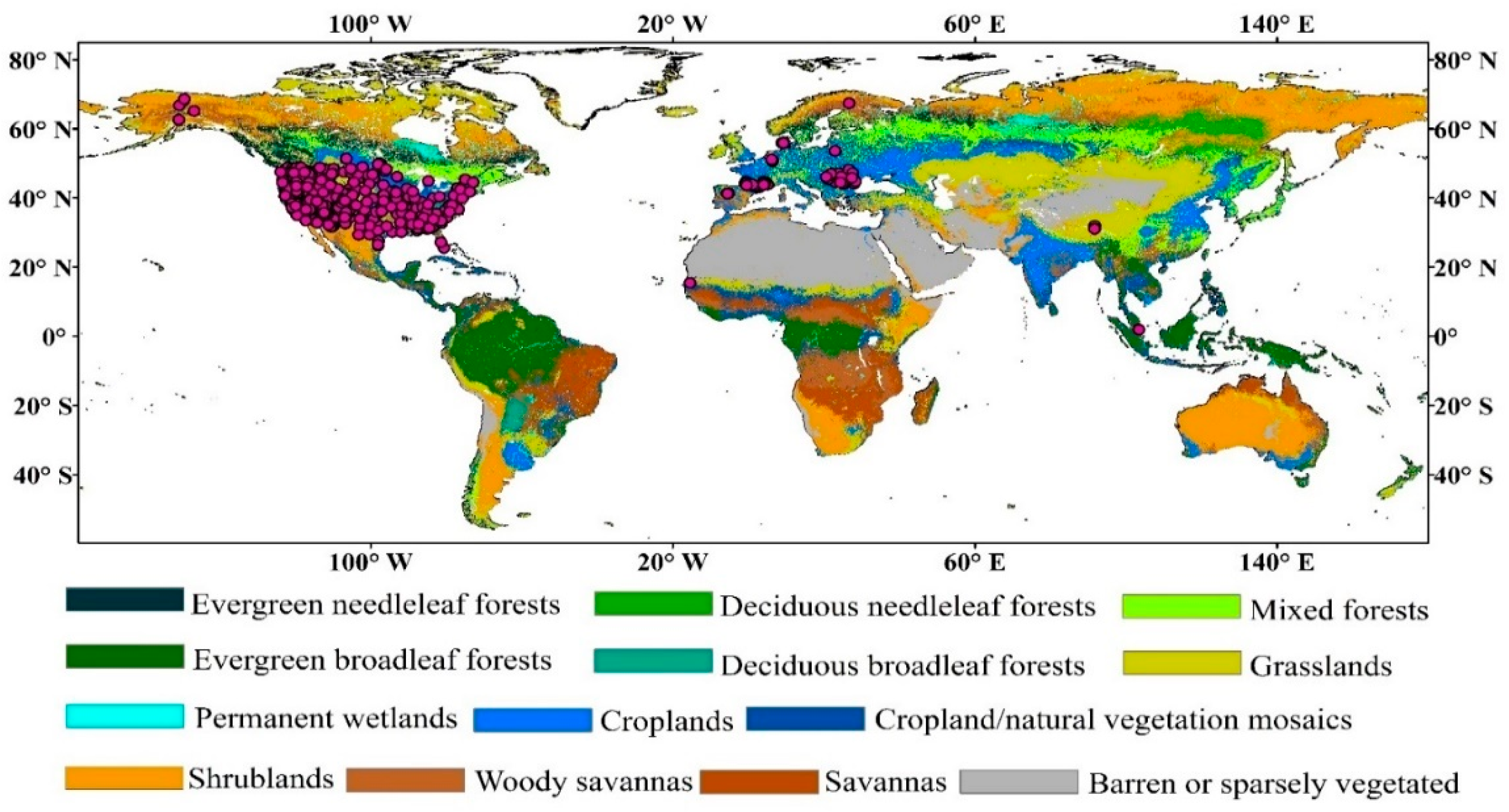
2.4. ISMN Ground-Based Soil Moisture

SMAP SM retrievals were also evaluated on a local scale against in situ SM datasets obtained from the ISMN network (International Soil Moisture Network) [44]. ISMN is an international initiative of GEWEX (Global Energy and Water Cycle Experiment) and ESA, aiming at the establishment and maintenance of a global in situ SM database. This database aims at promoting scientific studies on the validation and improvement of global satellite-based measurements and land surface modeling. Currently, the ISMN database hosts 2439 ground stations from ~60 networks (products are available at https://ismn.geo.tuwien.ac.at/). To ensure the accuracy of the ground-based observations and to minimize systematic discrepancies between in situ measurements and the SMAP SM retrievals, only SM observations of the top 0–5 cm soil layer flagged as “Good” were considered [45,46]. Consequently, 717 sites from 17 networks over the USA, Europe, Canada, China, and Africa were used. The spatial distribution of the in situ stations applied in our study are displayed in Figure 1 with a background of the International Geosphere-Biosphere Programme (IGBP) land cover classification.

2.5. Additional Datasets

Several additional datasets were used to interpret the results, including the International Geosphere-Biosphere Programme (IGBP) land cover classification scheme and MODIS leaf index area (LAI). Earlier studies have shown that the performance of the satellite-based SM products may vary as a function of vegetation density and land cover class [29,42,47]. Here, we used the IGBP land cover classification scheme and LAI data to account for the different land cover types and vegetation conditions when comparing the SM retrievals. In this study, the global land cover classification map is a 500 m resolution dataset obtained by overlapping the 10 years (2001–2012) standard MODIS land cover type product (MCD12Q1) using the IGBP schema [7,48]. It is generated, for each pixel, by choosing the highest overall confidence land cover classification from 2001 to 2010; more details are given in Broxton et al., 2014 [49]. The MODIS LAI product, over 2015–2017, was downloaded from NASA Earth Observations (NEO) websites (https://neo.sci.gsfc.nasa.gov/); it is a monthly LAI product calculated from MOD15A2 product and has a spatial resolution of 0.1 degrees. The global LAI map is obtained by the maximum value composite (MVC) method proposed by Holben [50]. All the additional data sets were rescaled to the resolution of 25 km, to ensure that all spatial data had the same spatial resolution.

3. Methodology

In our work we evaluated and inter-compared the performances of two SMAP SM retrievals against ECMWF modeled SM (global scale) and ground-based measurements (local scale) following three main rules: i) using a long period (i.e., April 2015–December 2017) of SM retrievals of each SMAP product as much as possible (until November 2019, MT-DCA was only updated to the end of 2017); ii) strictly using the same number of pixels (and thus of dates) between the two SMAP SM retrievals; iii) doing same data filtering, i.e., not recommended by the SMAP retrievals quality flag, SM values outside the range 0–0.6 m3/m3 [46], and temporal series of SMAP data pairs (i.e., number of observations available for validation) lower than one month (~31) were filtered out [51]. Four metrics, which are widely used in the soil moisture community [45,47], were used to compare the SMAP SM retrievals with the reference data (i.e., modeled ECMWF and in situ measurements): (Pearson) correlation coefficient (R; Equation 1) to assess the performance of SMAP retrievals to capture the seasonal variations of the reference SMs, bias (m3/m3; Equation 2) to measure the wetness or dryness of the SMAP SM compared to the reference SMs, root mean square difference (RMSD; m3/m3; Equation 3), and the ubRMSD (m3/m3; Equation 4) [18]. It should be noted that R and ubRMSD were considered as first-order criteria in comparison to Bias and RMSD, as the reference soil moisture datasets do not represent the value as “observed” by the SMAP measurement, considering the different “sampling” depths of simulated, retrieved and in-situ SM data.
R = i = 1 n ( SM est ( i ) SM est ¯ ) ( SM ref ( i ) SM ref ¯ ) i = 1 n ( SM est ( i ) SM est ¯ ) 2 i = 1 n ( SM ref ( i ) SM ref ¯ ) 2 ,
B i a s = ( SM est SM ref ) ¯ ,
R M S D = ( SM est SM ref ) 2 ¯ ,
u b R M S D = R M S D 2 B i a s 2 ,
where n is the number of SM data pairs, SMest is SMAP SM estimates (i.e., either SPL3SMP_E or MT-DCA SM), SMref is the reference SM (i.e., either ECMWF SM or ISMN in situ SM), and overbar represents the temporal mean of the entire time series. It should be noted that when comparing retrieved SM with in situ observations, the time series of satellite-based retrievals of SM were extracted from the original SMAP pixels covering each site (based on latitude and longitude of the site) to obtain values corresponding to the field measurements, and only the in situ data matching with the instantaneous overpass of the SMAP observation within a time window of 1 hour were selected. In our analysis, as done by Al-Yaari et al. (2019) [29], we accounted only for SM retrievals where p-value < 0.05 and R > 0.4 when comparing to in situ data sets (this condition only applies to the local scale evaluation). As correlation coefficients (R) cannot be simply averaged, we computed the median of R. In our analysis, in addition to the median skill metrics, we considered the spatial standard deviation.

4. Results

In the following parts, we described the validation results for two SMAP SM products on a global scale in Section 4.1. This involved directly interpreting the validation results compared to the ECMWF reanalysis SM and analyzing the effects of LAI and land cover types on the validation. Section 4.2 presents the validation results using the ground-based measurements.

4.1. Evaluation on a Global Scale

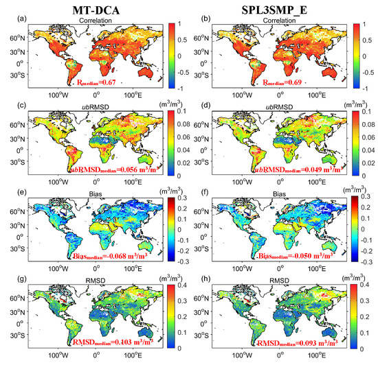
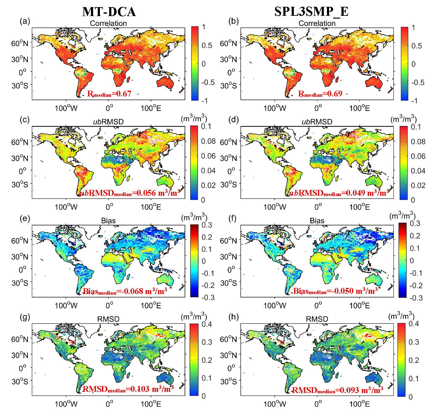
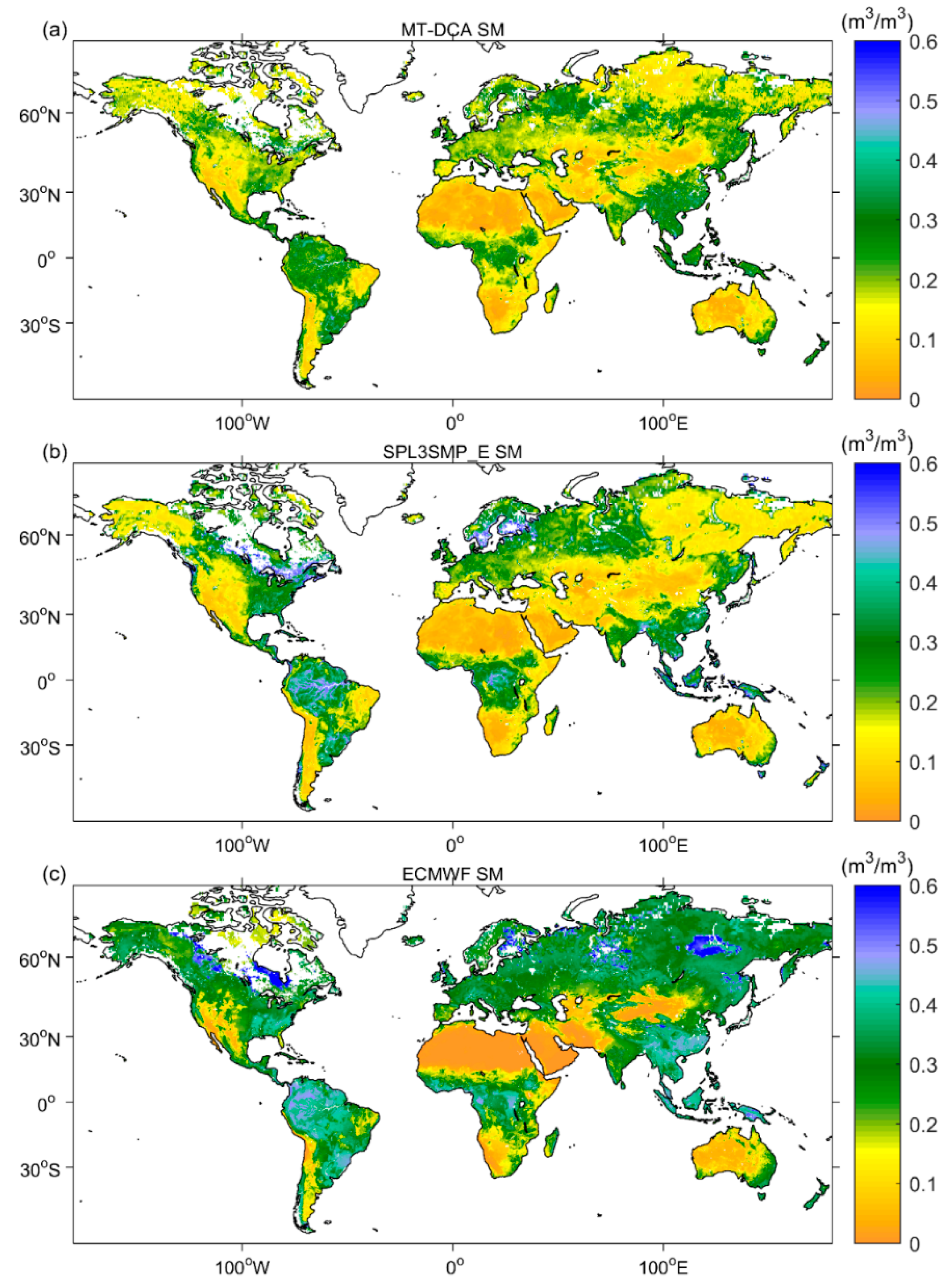
4.1.1. Validations Based on ECMWF Reanalysis SM

The results of comparing (i) SPL3SMP_E and (ii) MT-DCA SM retrievals with the modeled SM product obtained from the ECMWF reanalysis are shown in this part. The comparison was conducted spanning from April 2015 to December 2017 on a global scale. Figure 2 shows maps of the temporal mean SM values for the three SM datasets considered in this work. As mentioned in Section 2.3, the ECMWF modeled SM used here represents shallower soil surface (first 0–7 cm layer), and the inherent nature of this simulated SM is different from that observed by the SMAP satellite sensors. In contrast, the latter is more sensitive to soil surface depths of ~0–5 cm [18,23]. Hence, it should be mentioned that the ECMWF SM in Figure 2c must be interpreted according to spatial patterns rather than in terms of absolute values. As seen in Figure 2a,b, the spatial patterns of SM obtained by the MT-DCA have some differences with those obtained by SPL3SMP_E, although both are consistent with the spatial pattern of the ECMWF SM over most regions of the globe. The spatial patterns displayed by the ECMWF modeled SM are more consistent with SPL3SMP_E SM in some regions than with MT-DCA SM. For instance, MT-DCA SM shows to be relatively dry in some parts of the eastern US, while SPL3SMP_E SM is closer to ECMWF, as previous studies have indicated, these regions are wetter than the west and mid-west regions [52,53]. Some other regions (e.g., Amazon, Congo Basin) also present this similar spatial pattern. On the other hand, SPL3SMP_E SM was found to be relatively dry in the northern regions of China and the eastern regions of Russia, where MT-DCA SM is closer to ECMWF SM than SPL3SMP_E SM.
The metrics (i.e., R, ubRMSD, Bias, and RMSD) obtained from the direct comparison between MT-DCA and SPL3SMP_E with ECMWF SM are presented in Figure 3. In terms of correlation (R; Figure 3a,b), R values were found to be lower in forests than in other regions for both SMAP SM retrievals, and the two SMAP SM retrievals were negatively correlated with ECMWF SM over some specific forests, for instance, over the Congo and Amazon basins. Based on the values of ubRMSD and RMSD, large differences could be found. Specifically, the median ubRMSD (RMSD) computed on a global scale between MT-DCA and SPL3SMP_E SM retrievals against ECMWF SM were 0.056 m3/m3 (0.103 m3/m3) and 0.049 m3/m3 (0.093 m3/m3), respectively. Moreover, lower values were obtained for the SPL3SMP_E SM retrievals, especially over the tropical areas and western China (according to ubRMSD) and the eastern US (according to RMSD). ECMWF SM, in terms of Bias, is generally much wetter than SPL3SMP_E and MT-DCA SM retrievals, except for some arid and semi-arid regions (Sahara over northern Africa, and deserts over central Asia and Australia). However, SPL3SMP_E SM retrievals show a dry bias over some regions of the Amazon and Congo basin, which is opposite for MT-DCA SM retrievals. This can be explained in part by the discrepancies between the sampling depth of the modeled ECMWF SM data (0–7 cm top soil layer) and the SMAP SM data (~0–5 cm top soil layer) [47,52]. With this in mind, the different soil moisture Bias patterns presented in Figure 3e,f should be interpreted carefully.
As mentioned in Section 3, correlation and ubRMSD were regarded as primary quality criteria in this study. Thus, Figure 4 focuses on the spatial distribution of pixels with the best (highest) temporal correlation (R) and best (lowest) ubRMSD values attained when comparing ECMWF modeled SM either with MT-DCA SM (red) or SPL3SMP_E SM (blue) during April 2015–December 2017. The pixels where the result between MT-DCA SM and SPL3SMP_E SM differs by less than 0.02 in terms of correlation and less than 0.005 m3/m3 in terms of ubRMSD are indicated by a green color [52]. It was found that the red color is mainly distributed in the high latitudes of the northern part of the globe, meaning that MT-DCA is generally closer to ECMWF SM in regard to the time dynamics (R) in these regions. However, over most of the globe, SPL3SMP_E SM retrievals (blue areas) are performing better in terms of ubRMSD. It should also be mentioned that, in this figure, we only presented pixels with significant correlation (i.e., p < 0.05 and temporal series of data pairs >30).
The spatial distribution discrepancies between SPL3SMP_E and MT-DCA SM for bias or ubRMSD are shown in Figure 5. It can be found that the areas with large differences in bias are mainly covered by forests (e.g., Congo, Amazon Basin, and Boreal forests). In these regions, the difference for ubRMSD values is also higher, especially in western China.

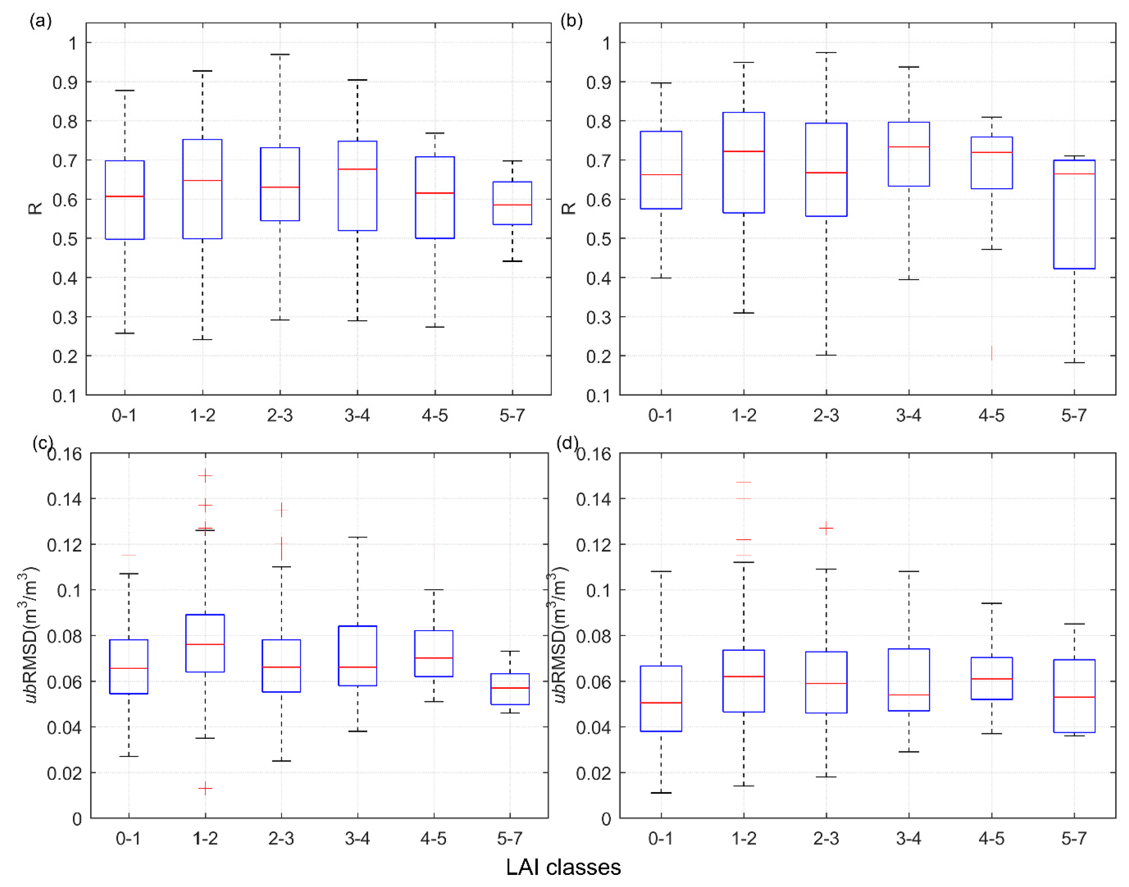
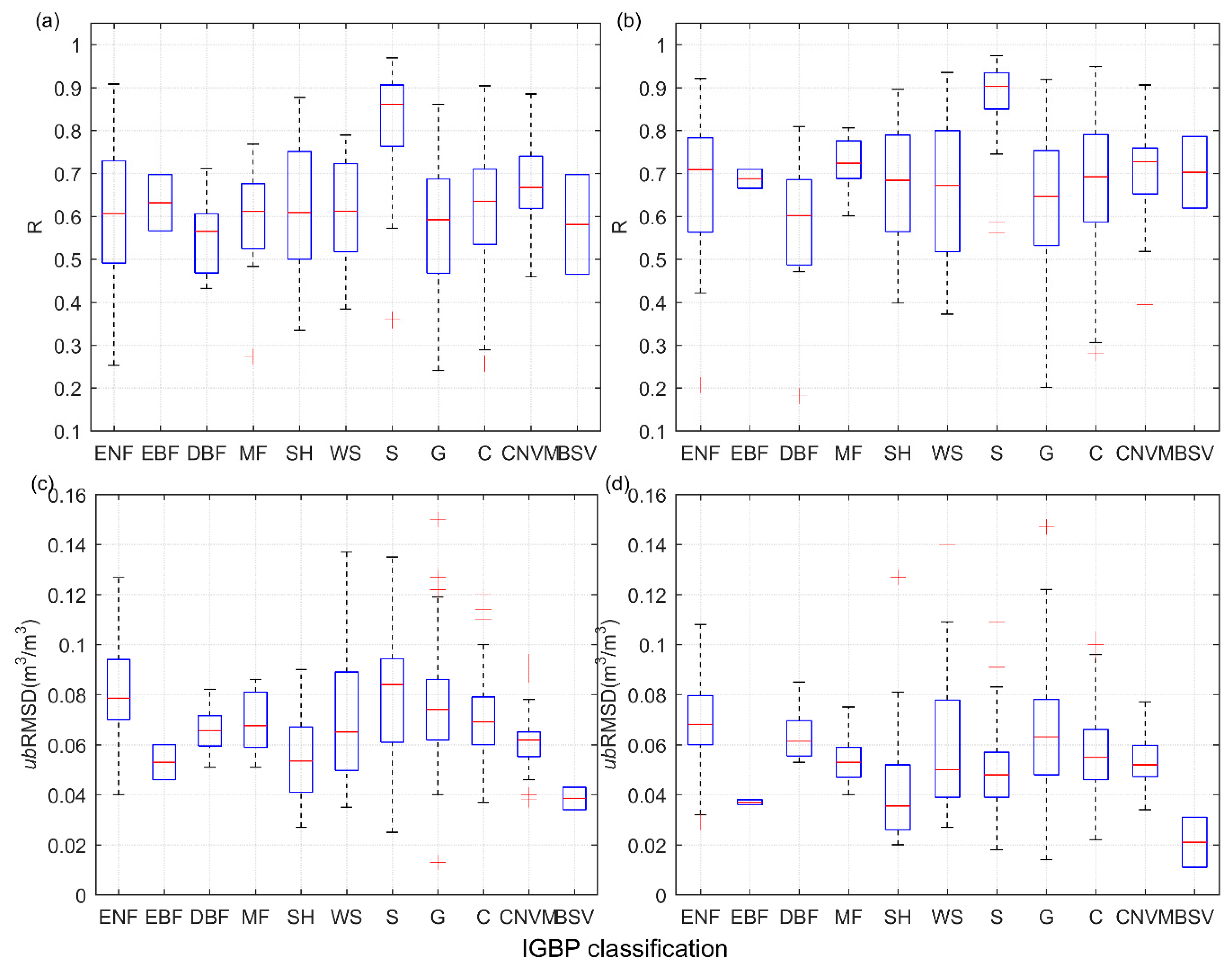
4.1.2. Impact of LAI and Land Cover Types

It is generally accepted by the SM community that land cover types affect the quality of satellite-based SM products [20,54], and earlier studies have shown that the performance of the satellite-based SM products may vary as a function of vegetation density and land cover type [29,42,47]. Hence, this part aims to evaluate and inter-compare the two SMAP SM retrievals for different vegetation conditions. The median values of the statistics (i.e., R and ubRMSD) obtained between ECMWF SM and both SMAP SM retrievals for LAI values ranging from 0 to 7 m2/m2 with an interval of 1 m2/m2 are presented in Figure 6. It can be found that there is a decrease in correlation (R) and an increase in ubRMSD for both SMAP SM retrievals with the increasing density of vegetation. Overall, SPL3SMP_E SM is better than (higher R values and lower ubRMSD values) MT-DCA SM for all LAI categories. According to correlation (R), small differences were obtained for MT-DCA and SPL3SMP_E SM for the categories 0–1, 1–2, 2–3, but the advantage of SPL3SMP_E SM is more obvious (the difference of R values > 0.02) when we are going from categories 4–5 to 5–7. According to Figure 6b, the ubRMSD obtained with SPL3SMP_E SM is lower than that obtained for MT-DCA SM for all LAI categories, with the category 5–7 being the most obvious (the difference of ubRMSD values > 0.01 m3/m3).
Figure 7 shows the same median metrics (R and ubRMSD) for MT-DCA and SPL3SMP_E SM, for all pixels stratified with the IGBP land cover type. In terms of correlation, it was found that the R values obtained with both retrieved SMAP SM retrievals over forest categories (except for “Deciduous broadleaf forests”) are lower than the R values over non forest categories (e.g., “Woody savannas”, ”Savannas”, and “croplands”). Except for “Mixed forests”, “Evergreen needleleaf forests”, and “Deciduous needleleaf forests”, the R values obtained with SPL3SMP_E SM are higher than that obtained for MT-DCA SM for all other land cover types, with results over the land type “Woody savannas” being the most obvious. In terms of ubRMSD, both MT-DCA and SPL3SMP_E SM have relatively low values over the “Shrublands” and “Barren or sparsely vegetated” compared to the other land surface types. It can be noted that SPL3SMP_E SM performs better (with lower ubRMSD) than MT-DCA SM for all land cover types, with best results (the difference of ubRMSD values > 0.01 m3/m3) over the land types “Evergreen broadleaf forests”, ”Mixed forests”, and “Deciduous needleleaf forests”.

4.2. Evaluation at the Local Scale

As a complement to Section 4.1 (i.e., compared to the ECMWF global reanalysis SM), the performance of MT-DCA SM and SPL3SMP_E SM was also compared to SM observed at 717 in situ sites from the ISMN networks during April 2015–December 2017. An overview of the performance of MT-DCA SM and SPL3SMP_E SM over the selected networks is presented in Table 2. In the latter table, the median values of all metrics are given for each measurement network. From the table, we found that the highest correlation values (R) for both MT-DCA and SPL3SMP_E SM obtained for network SOILSCAPE, while the lowest ones were found over the iRON network, with both R values lower than 0.50. For the other networks (except the FMI, TERENO, and iRON), SPL3SMP_E SM performs better than MT-DCA SM in terms of correlation. Being consistent with the results of the previous sections, according to the values of ubRMSD, SPL3SMP_E SM performs better than MT-DCA SM for all networks except in the iRON network where both MT-DCA and SPL3SMP_E SM retrievals are comparable.
According to median values calculated for all sites (“all” items in the last row of Table 2), a lower value of ubRMSD and a higher value of correlation was obtained for SPL3SMP_E SM (median ubRMSD of 0.070 m3/m3 for MT-DCA SM and 0.058 m3/m3 for SPL3SMP_E SM; median correlation of 0.63 for MT-DCA SM and 0.70 for SPL3SMP_E SM). Previous studies have shown that the Single Channel Algorithm using the V-polarized TB orbit (SCA-V) performed best in five alternative algorithms for SMAP soil moisture retrieval (the other four are SCA-H (using the H-polarized TB orbit as input), dual-channel algorithm(DCA), extend-DCA, and land parameter retrieval model) [21]. We have confirmed this again in this study, although it is MT-DCA, an improved DCA algorithm. MT-DCA SM and SPL3SMP_E SM had biases (remotely sensed data minus in-situ data) with the same sign (either positive or negative) over all networks except over the HOBE, SCAN, USCRN, and iRON networks. It should also be noted that the comparison with in-situ is carried out on the 9 km satellite footprint that covers a wider range of land cover types over the globe, which is very close to the overall validation results of Zhang et al. (2019) for SPL3SMP_E SM using ground measurements under various landscapes, and their reporting accuracy (i.e., unbiased RMSD) was equal to 0.055 m3/m3.
As in Section 4.1.2, in this part, we also evaluated (mainly based on R and ubRMSD) the two SMAP SM retrievals under different vegetation conditions (based either on LAI or IGBP land cover types). Figure 8 shows the median temporal correlation and unbiased RMSD computed between both SMAP SM products and in situ measurements, stratified based on LAI categories. It can be seen that, unlike the trend observed in Figure 6, both SMAP SM retrievals performed better even in the high LAI value category when compared to in situ measurements (both R and ubRMSD). In terms of temporal correlation (R), we found that the highest R values for both MT-DCA and SPL3SMP_E SM obtained for the category 3–4, the values are 0.68 and 0.73, respectively, of which SPL3SMP_E is higher. When compared to Figure 8a,b, SPL3SMP_E SM performs better than MT-DCA SM for all LAI categories. Specifically, the R value of SPL3SMP_E SM is higher than 0.6 (and close to 0.7) for all categories, while MT-DCA is close to or lower than 0.6. When focusing on ubRMSD, SPL3SMP_E SM yields the lowest value in category 0–1, while MT-DCA is in category 5–7. Except for LAI category 5–7, the ubRMSD values of MT-DCA SM are all higher than 0.06 m3/m3, while SPL3SMP_E SM is basically lower or close to this value. In contrast, SPL3SMP_E SM is closer to the SMAP soil moisture mission requirement [18].
Another insight into the effect of vegetation on the assessment of remotely-sensed soil moisture products using field measurements is shown in Figure 9. According to correlation, it was found that the temporal correlation of both SM retrievals showed the worst performance over “Deciduous broadleaf forests”, and their values are all lower than 0.60. Conversely, they performed best over “Savannas”, with R values approaching 0.90. The R values obtained with SPL3SMP_E are better than that of MT-DCA for all land cover categories, with best results (the difference of R values is greater than 0.1) over the land covers “Mixed forests”, “Evergreen needleleaf forests”, and “Barren or sparsely vegetated”. From Figure 9a,b, R of SPL3SMP_ES M generally fluctuates around ~0.7, while MT-DCA SM fluctuates around ~0.6 for all land cover types. In terms of ubRMSD, both MT-DCA and SPL3SMP_E have relatively low values over the “Evergreen broadleaf forests”, “Shrublands”, and “Barren or sparsely vegetated” categories compared to the other land surface types. It can be noted that the ubRMSD obtained with SPL3SMP_E is lower than that obtained with MT-DCA for all land cover types, with results over the land types “Evergreen broadleaf forests”, “Shrublands”, “Savannas”, and “Barren or sparsely vegetated” being the most obvious.

5. Discussions

Based on the evaluation results shown above in Figure 6, Figure 7, Figure 8 and Figure 9, it was found that comparing satellite-based SM retrievals to reference SMs (i.e., modeled ECMWF and in situ measurements) under different LAI classes or IGBP land cover types can impact the evaluation scores and the ranking of the two SMAP SM retrievals, due to different vegetation conditions. This is in line with previous evaluation studies on other satellite (e.g., SMOS (Soil Moisture and Ocean Salinity)) SM products [29,42,47] or other SMAP SM products [17,26,28]. On the one hand, considering different levels of LAI values compared to the reference SMs, SPL3SMP_E SM gave the best performance in terms of both correlations and ubRMSD, while on the other hand, MT-DCA SM performed better than SPL3SMP_E SM over “Mixed forests”, “Evergreen needleleaf forests”, and “Deciduous needleleaf forests” in terms of correlations when considering different IGBP land cover types compared to ECMWF modeled SM.
The performance, particularly in terms of temporal dynamics (R) and ubRMSD, of both SMAP SM retrievals, is better in low vegetation coverage areas (with higher R values and lower ubRMSD) than in high vegetation coverage areas (with lower R values and higher ubRMSD). This is probably due to the fact that SMAP operates at L-band [18]. In contrast, this band is more likely to penetrate areas with low vegetation coverage than areas with high vegetation coverage. It should be noted that the results obtained when comparing SMAP SM retrievals with ECMWF reanalysis SM and in situ observations are not the same, which does not mean that the results in our paper are contradictory. For instance, the rankings of the two SMAP SMs over “Mixed forests” and “Evergreen needleleaf forests” are opposite when compared with different reference SMs. This can be explained by the representative error of the sparse network. In addition, the sampling depth of reference SMs (0–7 cm top soil layer for the modeled ECMWF SM data; 0–5 cm top soil layer for in situ observations) and SM retrievals obtained from SMAP radiometer sensors (~0–5 cm top soil layer) is also different.
Although the absolute of bias between remotely-sensed SM products and in situ SM is very common due to many factors (e.g., representativeness errors between the point-scale in situ observations and coarse-resolution satellite-based products, spatial heterogeneity, different sensing depths (and thus observed volume), in situ sensor uncertainties, and even the auxiliary variables used in the SM inversion models) [29,55,56,57], this bias problem is not very obvious in this study when we look at “all” items in the last row of Table 2. However, this issue is very prominent (|Bias| even > 0.1 m3/m3) when doing an evaluation against sparse networks (the “Bias” column in Table 2), and the corresponding unbiased RMSD value is also larger than the target uncertainty of 0.04 m3/m3, which is mainly caused by representativeness errors [29].
In fact, not only the vegetation conditions, but also other factors including soil types, climatic zones, soil properties, VOD, surface roughness, and even different continents, are all worth analyzing in terms of their effects on soil moisture assessment [17,29,47]. However, we cannot solve all problems in one manuscript. The ultimate goal of this paper is to achieve the evaluation of the three-parameter inversion algorithm MT-DCA soil moisture products because although this algorithm uses multi-temporal observations and dual-polarized SMAP TB to achieve the simultaneous inversion of SM and VOD, due to too many unknown parameters (another parameter is effective scattering albedo), it also increases the uncertainty of the results [20]. Therefore, reducing the number of inversion parameters and replacing them with optimized parameters as the input should be a priority for future generations of MT-DCA retrieval algorithms.

6. Conclusions

The evaluation and inter-comparison of two SMAP SM retrievals (i.e., SPL3SMP_E and MT-DCA) were conducted in this work. We inter-compared the SMAP SM retrievals against the ECMWF modeled SM and ISMN ground-based measurements for different vegetation conditions at both global and local scales. The evaluation and inter-comparison were based on the correlation coefficient (R), RMSD, bias, and unbiased RMSD (ubRMSD) metrics. The results presented above can lead to several main conclusions:
(i)
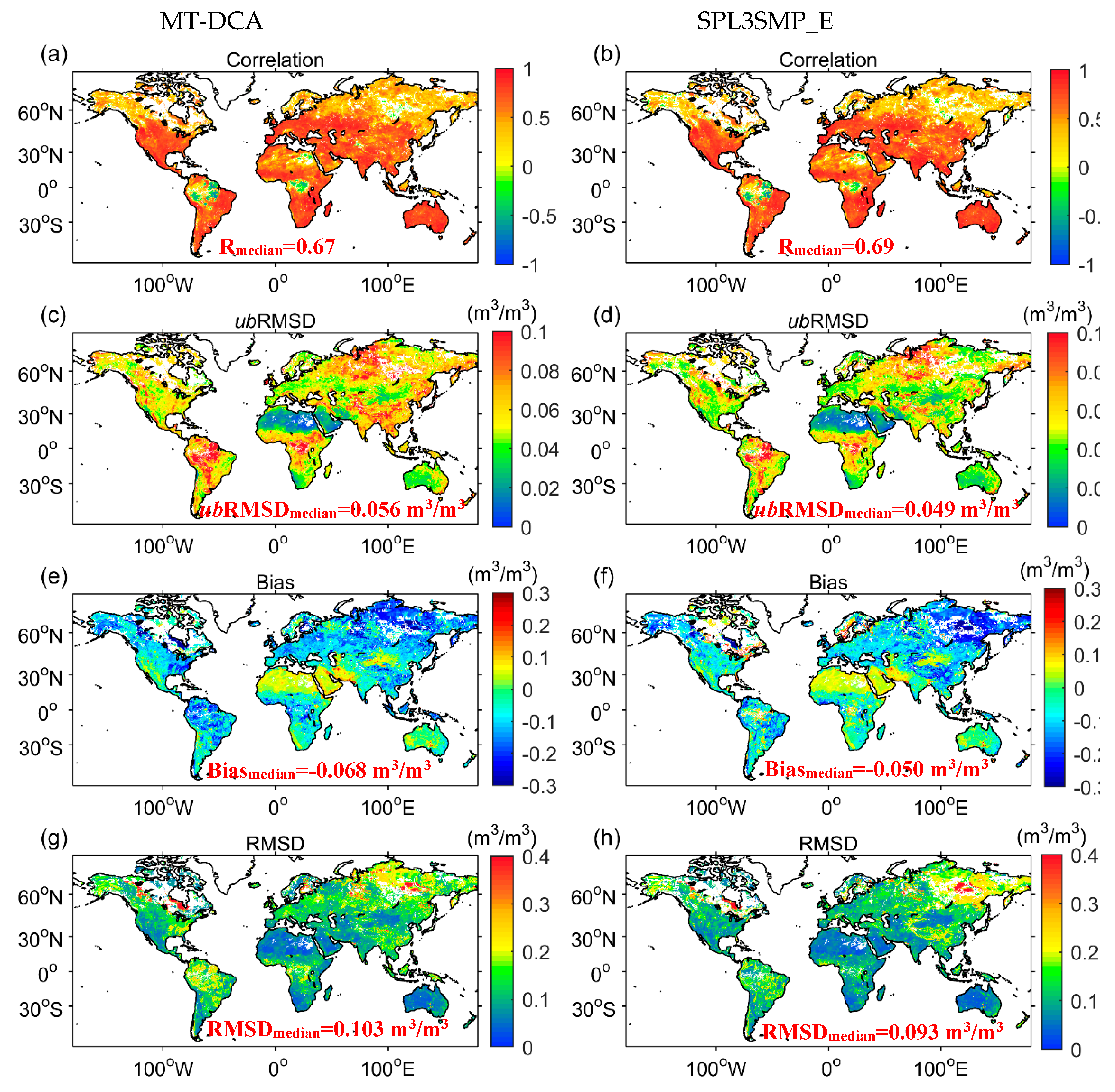
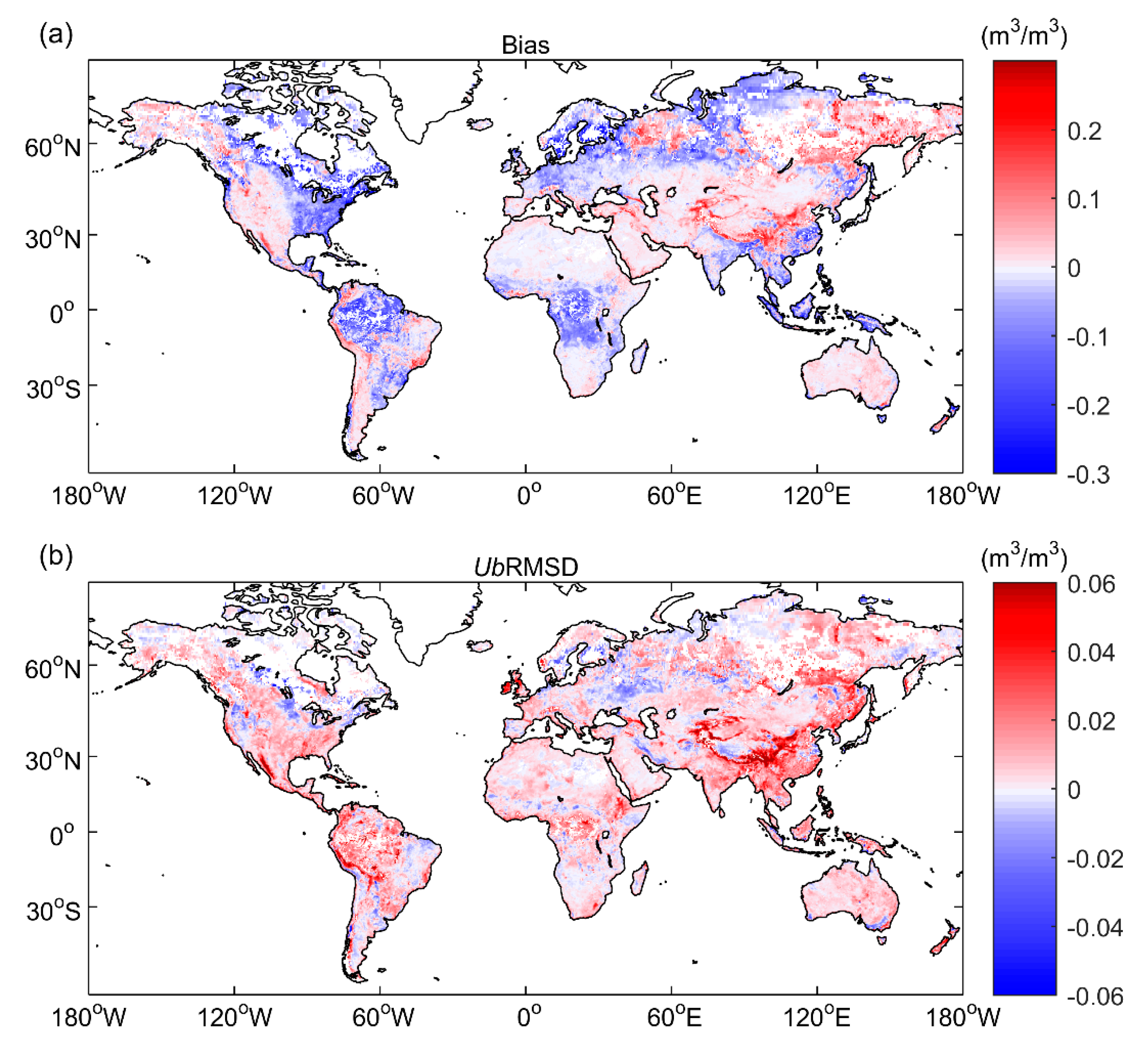
Both SPL3SMP_E and MT-DCA SM retrievals are generally found to be drier than ECMWF modeled SM, while MT-DCA SM was found to be drier than SPL3SMP_E SM by ~0.018 m3/m3 on average on a global scale. However, the different sampling layers considered for ECMWF modeled SM, in situ SM, and for the SMAP SM retrievals, makes it difficult to accurately evaluate the performance of the SMAP retrievals based on bias [52].
(ii)
Both SPL3SMP_E and MT-DCA SM retrievals can better capture the seasonal variations of ECMWF SM and in situ measurements. Specifically, the median R values computed on a global scale between SPL3SMP_E and MT-DCA SM against ECMWF SM were 0.69 and 0.67, respectively, while the median correlation of SPL3SMP_E and MT-DCA SM with in situ measurements computed over all ISMN sites were 0.70 and 0.63, respectively.
(iii)
The ubRMSD obtained with SPL3SMP_E is always lower than that obtained with MT-DCA. Specifically, the median ubRMSD values computed on a global scale between SPL3SMP_E and MT-DCA SM against ECMWF SM were 0.049 m3/m3 and 0.056 m3/m3, respectively, while the median ubRMSD of SPL3SMP_E and MT-DCA SM with in situ measurements computed over all ISMN sites were 0.058 m3/m3 and 0.070 m3/m3, respectively.
(iv)
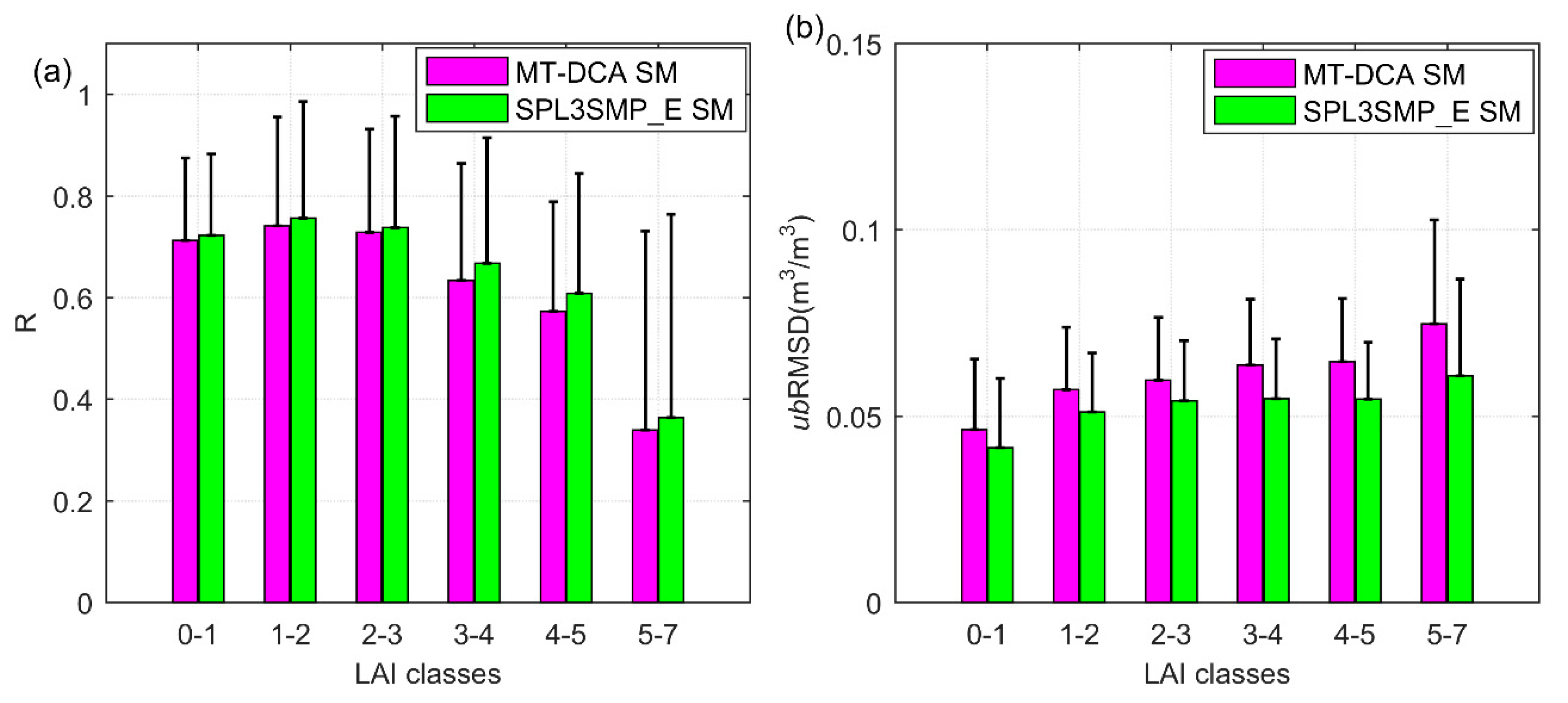
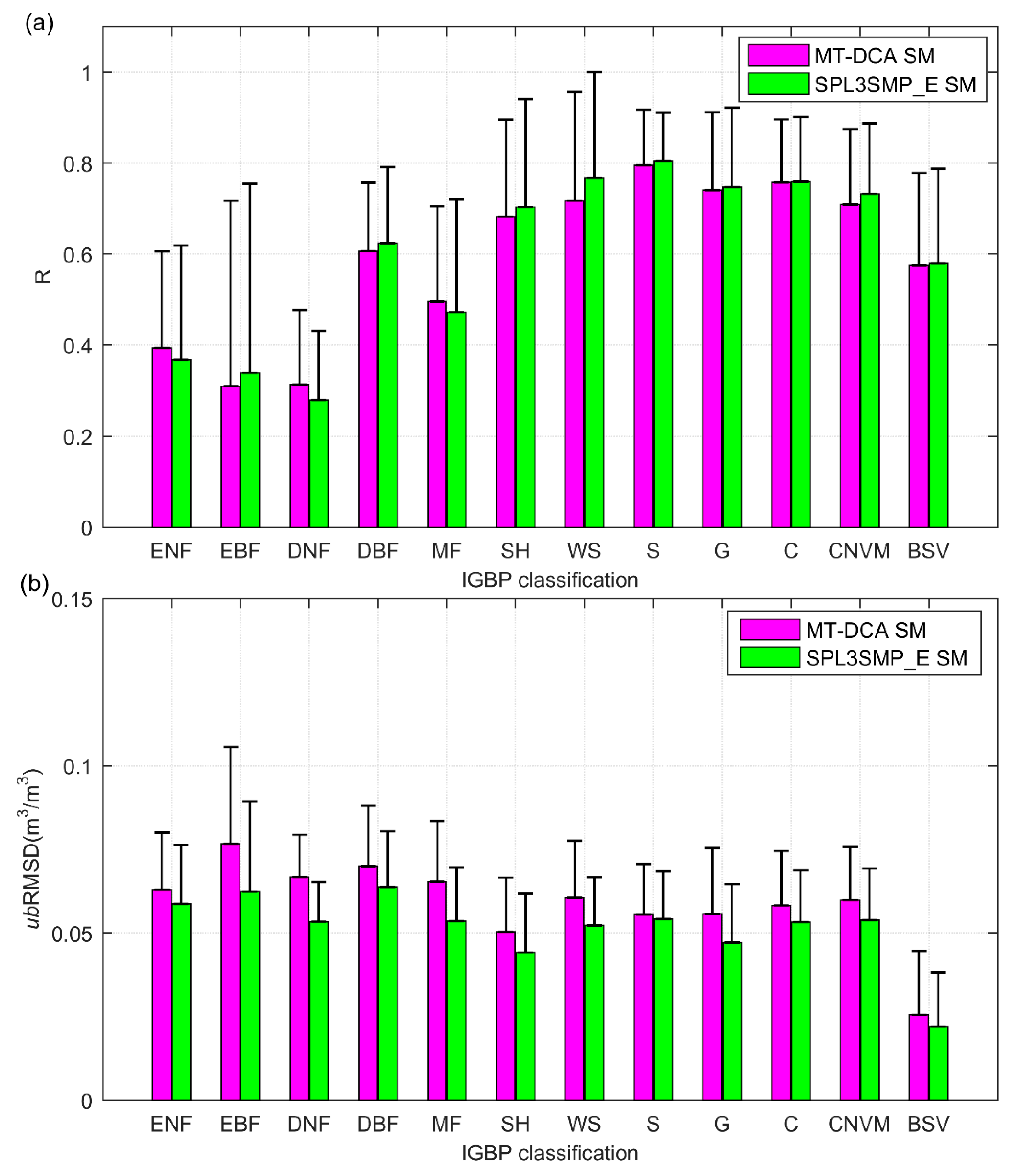
The R values (ubRMSD) obtained with SPL3SMP_E is always higher (lower) than that obtained with MT-DCA over all LAI categories or IGBP land cover types when compared either to the ECMWF modeled SM or in situ SM measurements.
As summarized above, retrieved SM achieved with the SPL3SMP_E (SCA-V) is always better than that achieved with MT-DCA according to temporal correlations and ubRMSD, which were regarded as primary quality criteria in this study. It is one of the first times a study has shown that the SCA-V algorithm delivered better retrieval performance than MT-DCA, an improved DCA algorithm. It also fills the gap in understanding whether MT-DCA SM meets the accuracy requirements of the SMAP mission (i.e., 0.04 m3/m3). Furthermore, there is very little known about the performance of SMAP-enhanced level three SM products at different vegetation conditions. Thus, our study is also complementary to the evaluation of this soil moisture products by Zhang et al. (2019) [17].

Author Contributions

X.L. (Xin Lv) and X.L. (Xiaojun Li) provided the ideas for this work; L.B. and X.L. (Xiaojun Li) designed and performed the experiments; L.B. and X.L. (Xin Lv) collected and processed the data; L.B. wrote the paper. These authors contributed equally.

Funding

This work was funded by the Major scientific and technological projects of Xinjiang Production and Construction Corps (2018AA004). Xiaojun Li was sponsored by China Scholarship Council (201804910838).

Acknowledgments

We are grateful to Alexandra G. Konings, Assistant Professor, from the Department of Earth System Science, Stanford University for providing the MT-DCA data. We would like to thank people who participated in the ISMN campaign. We also thank the reviewers for their constructive suggestions.

Conflicts of Interest

The authors declare no conflict of interest.

Appendix A

Table A1. Specific values of median metrics (R and ubRMSD, m3/m3) in Figure 6.
LAI Classes R(SD)ubRMSD(SD) (m3/m3)
MT-DCASPL3SMP_E MT-DCASPL3SMP_E
0–10.71(0.162)0.72(0.161)0.046(0.019)0.042(0.019)
1–20.74(0.213)0.76(0.229)0.057(0.017)0.051(0.016)
2–30.73(0.203)0.74(0.219)0.060(0.017)0.054(0.016)
3–40.63(0.231)0.67(0.247)0.064(0.018)0.055(0.016)
4–50.57(0.216)0.61(0.236)0.065(0.017)0.055(0.015)
5–70.34(0.392)0.36(0.400)0.075(0.028)0.061(0.026)
Table A2. Specific values of median metrics (R and ubRMSD, m3 / m3) in Figure 7.
IGBP ClassificationR(SD)ubRMSD(SD) (m3/m3)IGBP ClassificationR(SD)ubRMSD(SD) (m3/m3)
MT-DCASPL3SMP_E MT-DCASPL3SMP_E MT-DCASPL3SMP_E MT-DCASPL3SMP_E
ENF0.39(0.213)0.37(0.251)0.063(0.017)0.059(0.018)WS0.72(0.239)0.77(0.233)0.061(0.017)0.052(0.014)
EBF0.31(0.407)0.34(0.415)0.077(0.029)0.062(0.027)SH0.79(0.122)0.80(0.106)0.056(0.015)0.054(0.014)
DNF0.31(0.164)0.28(0.152)0.067(0.012)0.053(0.012)G0.74(0.171)0.75(0.175)0.056(0.020)0.047(0.017)
DBF0.61(0.150)0.62(0.168)0.07(0.018)0.064(0.017)C0.76(0.137)0.76(0.142)0.058(0.016)0.053(0.015)
MF0.50(0.208)0.47(0.249)0.065(0.018)0.054(0.016)CNVM0.71(0.165)0.73(0.154)0.06(0.016)0.054(0.015)
SH0.68(0.212)0.70(0.236)0.05(0.016)0.044(0.018)BSV0.58(0.203)0.58(0.208)0.026(0.019)0.022(0.016)
Note: the abbreviation of the IGBP classification is the same as that of Figure 7.

References

  1. Koster, R.D.; Dirmeyer, P.A.; Guo, Z.; Bonan, G.; Chan, E.; Cox, P.; Gordon, C.T.; Kanae, S.; Kowalczyk, E.; Lawrence, D.; et al. Regions of Strong Coupling between Soil Moisture and Precipitation. Science 2004, 305, 1138–1140. [Google Scholar] [CrossRef] [PubMed] [Green Version]
  2. Li, X.; Xin, X.; Jiao, J.; Peng, Z.; Zhang, H.; Shao, S.; Liu, Q. Estimating Subpixel Surface Heat Fluxes through Applying Temperature-Sharpening Methods to Modis Data. Remote Sens. 2017, 9, 836. [Google Scholar] [CrossRef] [Green Version]
  3. Seneviratne, S.I.; Corti, T.; Davin, E.L.; Hirschi, M.; Jaeger, E.B.; Lehner, I.; Orlowsky, B.; Teuling, A.J. Investigating Soil Moisture–Climate Interactions in a Changing Climate: A Review. Earth Sci. Rev. 2011, 99, 125–161. [Google Scholar] [CrossRef]
  4. Wu, T.; Fan, M.; Tao, J.; Su, L.; Wang, P.; Liu, D.; Li, M.; Han, X.; Chen, L. Aerosol Optical Properties over China from Rams-Cmaq Model Compared with Caliop Observations. Atmosphere 2017, 8, 201. [Google Scholar] [CrossRef] [Green Version]
  5. Hao, D.; Asrar, G.R.; Zeng, Y.; Zhu, Q.; Wen, J.; Xiao, Q.; Chen, M. Estimating Hourly Land Surface Downward Shortwave and Photosynthetically Active Radiation from Dscovr/Epic Observations. Remote Sens. Environ. 2019, 232, 111320. [Google Scholar] [CrossRef]
  6. Chen, T.; McVicar, T.; Wang, G.; Chen, X.; de Jeu, R.; Liu, Y.; Shen, H.; Zhang, F.; Dolman, A. Advantages of Using Microwave Satellite Soil Moisture over Gridded Precipitation Products and Land Surface Model Output in Assessing Regional Vegetation Water Availability and Growth Dynamics for a Lateral Inflow Receiving Landscape. Remote Sens. 2016, 8, 428. [Google Scholar] [CrossRef] [Green Version]
  7. Li, X.; Xin, X.; Peng, Z.; Zhang, H.; Li, L.; Shao, S.; Liu, Q. Estimation of Land Surface Heat Fluxes Based on Visible Infrared Imaging Radiometer Suite Data: Case Study in Northern China. J. Appl. Remote Sens. 2017, 11, 046012. [Google Scholar] [CrossRef] [Green Version]
  8. Miralles, D.G.; Teuling, A.J.; Van Heerwaarden, C.C.; De Arellano, J.V.G. Mega-Heatwave Temperatures Due to Combined Soil Desiccation and Atmospheric Heat Accumulation. Nat. Geosci. 2014, 7, 345. [Google Scholar] [CrossRef]
  9. Miralles, D.G.; Van Den Berg, M.J.; Gash, J.H.; Parinussa, R.M.; De Jeu, R.A.; Beck, H.E.; Holmes, T.R.; Jiménez, C.; Verhoest, N.E.; Dorigo, W.A.; et al. El Niño–La Niña Cycle and Recent Trends in Continental Evaporation. Nat. Clim. Chang. 2014, 4, 122. [Google Scholar] [CrossRef]
  10. Pitman, A.J. The Evolution of, and Revolution in, Land Surface Schemes Designed for Climate Models. Int. J. Climatol. A J. R. Meteorol. Soc. 2003, 23, 479–510. [Google Scholar] [CrossRef]
  11. Li, X.; Xin, X.; Peng, Z.; Yi, C.; Li, B. Analysis of the Spatial Variability of Land Surface Variables for ET Estimation: Case Study in HiWATER Campaign. Remote Sens. 2018, 10, 91. [Google Scholar] [CrossRef] [Green Version]
  12. Carrão, H.; Russo, S.; Sepulcre-Canto, G.; Barbosa, P. An Empirical Standardized Soil Moisture Index for Agricultural Drought Assessment from Remotely Sensed Data. Int. J. Appl. Earth Obs. Geoinf. 2016, 48, 74–84. [Google Scholar] [CrossRef]
  13. Roy, S.K.; Rowlandson, T.L.; Berg, A.A.; Champagne, C.; Adams, J.R. Impact of Sub-Pixel Heterogeneity on Modelled Brightness Temperature for an Agricultural Region. Int. J. Appl. Earth Obs. Geoinf. 2016, 45, 212–220. [Google Scholar] [CrossRef]
  14. Wang, Y.; Ni, W.; Sun, G.; Chi, H.; Zhang, Z.; Guo, Z. Slope-Adaptive Waveform Metrics of Large Footprint Lidar for Estimation of Forest Aboveground Biomass. Remote Sens. Environ. 2019, 224, 386–400. [Google Scholar] [CrossRef]
  15. Ciabatta, L.; Brocca, L.; Massari, C.; Moramarco, T.; Gabellani, S.; Puca, S.; Wagner, W. Rainfall-Runoff Modelling by Using Sm2rain-Derived and State-of-the-Art Satellite Rainfall Products over Italy. Int. J. Appl. Earth Obs. Geoinf. 2016, 48, 163–173. [Google Scholar] [CrossRef]
  16. Wei, J.; Huang, W.; Li, Z.; Xue, W.; Peng, Y.; Sun, L.; Cribb, M. Estimating 1-Km-Resolution Pm2. 5 Concentrations across China Using the Space-Time Random Forest Approach. Remote Sens. Environ. 2019, 231, 111221. [Google Scholar] [CrossRef]
  17. Zhang, R.; Kim, S.; Sharma, A. A Comprehensive Validation of the Smap Enhanced Level-3 Soil Moisture Product Using Ground Measurements over Varied Climates and Landscapes. Remote Sens. Environ 2019, 223, 82–94. [Google Scholar] [CrossRef]
  18. Entekhabi, D.; Njoku, E.G.; O’Neill, P.E.; Kellogg, K.H.; Crow, W.T.; Edelstein, W.N.; Entin, J.K.; Goodman, S.D.; Jackson, T.J.; Johnson, J. The Soil Moisture Active Passive (Smap) Mission. Proc. IEEE 2010, 98, 704–716. [Google Scholar] [CrossRef]
  19. Kerr, Y.H.; Waldteufel, P.; Wigneron, J.P.; Delwart, S.; Cabot, F.; Boutin, J.; Escorihuela, M.J.; Font, J.; Reul, N.; Gruhier, C.; et al. The Smos Mission: New Tool for Monitoring Key Elements Ofthe Global Water Cycle. Proc. IEEE 2010, 98, 666–687. [Google Scholar] [CrossRef] [Green Version]
  20. Wigneron, J.P.; Jackson, T.J.; O’neill, P.; De Lannoy, G.; De Rosnay, P.; Walker, J.P.; Ferrazzoli, P.; Mironov, V.; Bircher, S.; Grant, J.P.; et al. Modelling the Passive Microwave Signature from Land Surfaces: A Review of Recent Results and Application to the L-Band Smos & Smap Soil Moisture Retrieval Algorithms. Remote Sens. Environ. 2017, 192, 238–262. [Google Scholar]
  21. Chan, S.K.; Bindlish, R.; O’Neill, P.; Jackson, T.; Njoku, E.; Dunbar, S.; Chaubell, J.; Piepmeier, J.; Yueh, S.; Entekhabi, D.; et al. Development and Assessment of the Smap Enhanced Passive Soil Moisture Product. Remote Sens. Environ. 2018, 204, 931–941. [Google Scholar] [CrossRef] [Green Version]
  22. Chan, S.K.; Bindlish, R.; O’Neill, P.E.; Njoku, E.; Jackson, T.; Colliander, A.; Chen, F.; Burgin, M.; Dunbar, S.; Piepmeier, J.; et al. Assessment of the Smap Passive Soil Moisture Product. IEEE Trans. Geosci. Remote Sens. 2016, 25, 4994–5007. [Google Scholar] [CrossRef]
  23. Colliander, A.; Jackson, T.J.; Bindlish, R.; Chan, S.; Das, N.; Kim, S.B.; Cosh, M.H.; Dunbar, R.S.; Dang, L.; Pashaian, L. Validation of Smap Surface Soil Moisture Products with Core Validation Sites. Remote Sens. Environ. 2017, 191, 215–231. [Google Scholar] [CrossRef]
  24. Colliander, A.; Jackson, T.J.; Chan, S.K.; O’Neill, P.; Bindlish, R.; Cosh, M.H.; Caldwell, T.; Walker, J.P.; Berg, A.; McNairn, H.; et al. An Assessment of the Differences between Spatial Resolution and Grid Size for the Smap Enhanced Soil Moisture Product over Homogeneous Sites. Remote Sens. Environ. 2018, 207, 65–70. [Google Scholar] [CrossRef]
  25. Jackson, T.; O’Neill, P.; Chan, S.; Bindlish, R.; Colliander, A.; Chen, F.; Dunbar, S.; Piepmeier, J.; Misra, S.; Cosh, M.; et al. Calibration and Validation for the L2/3_Sm_P Version 5 and L2/3_Sm_P_E Version 2 Data Products. In Smap Project, Jpl D-56297; Jet Propulsion Laboratory: Pasadena, CA, USA, 2018. [Google Scholar]
  26. Kim, H.; Parinussa, R.; Konings, A.G.; Wagner, W.; Cosh, M.H.; Choi, M. Global-Scale Assessment and Combination of Smap with Ascat Active) and Amsr2 Passive) Soil Moisture Products. Remote Sens. Environ. 2018, 204, 260–275. [Google Scholar] [CrossRef]
  27. Pan, M.; Cai, X.; Chaney, N.W.; Entekhabi, D.; Wood, E.F. An Initial Assessment of Smap Soil Moisture Retrievals Using High-Resolution Model Simulations and in Situ Observations. Geophys. Res. Lett. 2016, 43, 9662–9668. [Google Scholar] [CrossRef] [Green Version]
  28. Tavakol, A.; Rahmani, V.; Quiring, S.M.; Kumar, S.V. Evaluation Analysis of Nasa Smap L3 and L4 and Sport-Lis Soil Moisture Data in the United States. Remote Sens. Environ. 2019, 229, 234–246. [Google Scholar] [CrossRef]
  29. Al-Yaari, A.; Wigneron, J.P.; Dorigo, W.; Colliander, A.; Pellarin, T.; Hahn, S.; Mialon, A.; Richaume, P.; Fernandez-Moran, R.; Fan, L.; et al. Assessment and Inter-Comparison of Recently Developed/Reprocessed Microwave Satellite Soil Moisture Products Using Ismn Ground-Based Measurements. Remote Sens. Environ. 2019, 224, 289–303. [Google Scholar] [CrossRef]
  30. Konings, A.G.; Piles, M.; Das, N.; Entekhabi, D. L-Band Vegetation Optical Depth and Effective Scattering Albedo Estimation from Smap. Remote Sens. Environ. 2017, 198, 460–470. [Google Scholar] [CrossRef]
  31. Dorigo, W.A.; Gruber, A.; De Jeu, R.A.M.; Wagner, W.; Stacke, T.; Loew, A.; Albergel, C.; Brocca, L.; Chung, D.; Parinussa, R.M.; et al. Evaluation of the Esa Cci Soil Moisture Product Using Ground-Based Observations. Remote Sens. Environ. 2015, 162, 380–395. [Google Scholar] [CrossRef]
  32. Dorigo, W.; Wagner, W.; Albergel, C.; Albrecht, F.; Balsamo, G.; Brocca, L.; Chung, D.; Ertl, M.; Forkel, M.; Gruber, A. Esa Cci Soil Moisture for Improved Earth System Understanding: State-of-the Art and Future Directions. Remote Sens. Environ. 2017, 203, 185–215. [Google Scholar] [CrossRef]
  33. Torres, R.; Snoeij, P.; Geudtner, D.; Bibby, D.; Davidson, M.; Attema, E.; Potin, P.; Rommen, B.; Floury, N.; Brown, M. Gmes Sentinel-1 Mission. Remote Sens. Environ. 2012, 120, 9–24. [Google Scholar] [CrossRef]
  34. Chaubell, J. Smap Algorithm Theoretical Basis Document: Enhanced L1b Radiometer Brightness Temperature Product. Jet Propulsion Laboratory, California Institute of Technology, Pasadena, CA (JPL D-56287). Available online: https://nsidc.org/sites/nsidc.org/files/technical-references/SMAP_L1B_TB_E_Product_ATBD_D-56287.pdf (accessed on 10 February 2017).
  35. Poe, G.A. Optimum Interpolation of Imaging Microwave Radiometer Data. IEEE Trans. Geosci. Remote Sens. 1990, 28, 800–810. [Google Scholar] [CrossRef] [Green Version]
  36. O’Neill, P.E.; Chan, S.; Njoku, E.G.; Jackson, T.; Bindlish, R. Smap Enhanced L3 Radiometer Global Daily 9 Km Ease-Grid Soil Moisture. Version 2.[SPL3SMP _ E]. Boulder, Colorado USA. NASA National Snow and Ice Data Center Distributed Active Archive Center. 2018. Available online: https://doi.org/10.5067/RFKIZ5QY5ABN (accessed on 18 September 2019).
  37. De Jeu, R.A.; Wagner, W.; Holmes, T.R.H.; Dolman, A.J.; Van De Giesen, N.C.; Friesen, J. Global Soil Moisture Patterns Observed by Space Borne Microwave Radiometers and Scatterometers. Surv. Geophys. 2008, 29, 399–420. [Google Scholar] [CrossRef] [Green Version]
  38. Konings, A.G.; Piles, M.; Rötzer, K.; McColl, K.A.; Chan, S.K.; Entekhabi, D. Vegetation Optical Depth and Scattering Albedo Retrieval Using Time Series of Dual-Polarized L-Band Radiometer Observations. Remote Sens. Environ. 2016, 172, 178–189. [Google Scholar] [CrossRef]
  39. Berrisford, P.; Kållberg, P.; Kobayashi, S.; Dee, D.; Uppala, S.; Simmons, A.J.; Poli, P.; Sato, H. Atmospheric Conservation Properties in Era-Interim. Q. J. R. Meteorol. Soc. 2011, 137, 1381–1399. [Google Scholar] [CrossRef]
  40. Dee, D.P.; Uppala, S.M.; Simmons, A.J.; Berrisford, P.; Poli, P.; Kobayashi, S.; Andrae, U.; Balmaseda, M.A.; Balsamo, G.; Bauer, D.P.; et al. The Era-Interim Reanalysis: Configuration and Performance of the Data Assimilation System. Q. J. R. Meteorol. Soc. 2011, 137, 553–597. [Google Scholar] [CrossRef]
  41. Albergel, C.; De Rosnay, P.; Gruhier, C.; Muñoz-Sabater, J.; Hasenauer, S.; Isaksen, L.; Kerr, Y.; Wagner, W. Evaluation of Remotely Sensed and Modelled Soil Moisture Products Using Global Ground-Based in Situ Observations. Remote Sens. Environ. 2012, 118, 215–226. [Google Scholar] [CrossRef]
  42. Al-Yaari, A.; Wigneron, J.P.; Ducharne, A.; Kerr, Y.H.; Wagner, W.; De Lannoy, G.; Reichle, R.; Al Bitar, A.; Dorigo, W.; Richaume, P.; et al. Global-Scale Comparison of Passive (Smos) and Active (Ascat) Satellite Based Microwave Soil Moisture Retrievals with Soil Moisture Simulations (Merra-Land). Remote Sens. Environ. 2014, 152, 614–626. [Google Scholar] [CrossRef] [Green Version]
  43. Fan, L.; Al-Yaari, A.; Frappart, F.; Swenson, J.J.; Xiao, Q.; Wen, J.; Jin, R.; Kang, J.; Li, X.; Fernandez-Moran, R. Mapping Soil Moisture at a High Resolution over Mountainous Regions by Integrating in Situ Measurements, Topography Data, and Modis Land Surface Temperatures. Remote Sens. 2019, 11, 656. [Google Scholar] [CrossRef] [Green Version]
  44. Dorigo, W.A.; Wagner, W.; Hohensinn, R.; Hahn, S.; Paulik, C.; Xaver, A.; Gruber, A.; Drusch, M.; Mecklenburg, S.; Oevelen, P.V.; et al. The International Soil Moisture Network: A Data Hosting Facility for Global in Situ Soil Moisture Measurements. Hydrol. Earth Syst. Sci. 2011, 15, 1675–1698. [Google Scholar] [CrossRef] [Green Version]
  45. Al-Yaari, A.; Wigneron, J.P.; Kerr, Y.; Rodriguez-Fernandez, N.; O’Neill, P.E.; Jackson, T.J.; De Lannoy, G.J.M.; Al Bitar, A.; Mialon, A.; Richaume, P.; et al. Evaluating Soil Moisture Retrievals from Esa’s Smos and Nasa’s Smap Brightness Temperature Datasets. Remote Sens. Environ. 2017, 193, 257–273. [Google Scholar] [CrossRef] [PubMed] [Green Version]
  46. Dorigo, W.A.; Xaver, A.; Vreugdenhil, M.; Gruber, A.; Hegyiova, A.; Sanchis-Dufau, A.D.; Zamojski, D.; Cordes, C.; Wagner, W.; Drusch, M.; et al. Global Automated Quality Control of in Situ Soil Moisture Data from the International Soil Moisture Network. Vadose Zone J. 2013, 12, vzj2012.0097. [Google Scholar] [CrossRef]
  47. Li, X.; Al-Yaari, A.; Schwank, M.; Fan, L.; Frappart, F.; Swenson, J.; Wigneron, J.P. Compared Performances of Smos-Ic Soil Moisture and Vegetation Optical Depth Retrievals Based on Tau-Omega and Two-Stream Microwave Emission Models. Remote Sens. Environ. 2020, 236, 111502. [Google Scholar] [CrossRef]
  48. Fan, L.; Wigneron, J.P.; Xiao, Q.; Al-Yaari, A.; Wen, J.; Martin-StPaul, N.; Dupuy, J.L.; Pimont, F.; Al Bitar, A.; Fernandez-Moran, R.; et al. Evaluation of Microwave Remote Sensing for Monitoring Live Fuel Moisture Content in the Mediterranean Region. Remote Sens. Environ. 2018, 205, 210–223. [Google Scholar] [CrossRef]
  49. Broxton, P.D.; Zeng, X.; Sulla-Menashe, D.; Troch, P.A. A Global Land Cover Climatology Using Modis Data. J. Appl. Meteorol. Climatol. 2014, 53, 1593–1605. [Google Scholar] [CrossRef]
  50. Holben, B.N. Characteristics of Maximum-Value Composite Images from Temporal Avhrr Data. Int. J. Remote Sens. 1986, 7, 1417–1434. [Google Scholar] [CrossRef]
  51. Kolassa, J.; Reichle, R.H.; Liu, Q.; Alemohammad, S.H.; Gentine, P.; Aida, K.; Asanuma, J.; Bircher, S.; Caldwell, T.; Colliander, A.; et al. Estimating Surface Soil Moisture from Smap Observations Using a Neural Network Technique. Remote Sens. Environ. 2018, 204, 43–59. [Google Scholar] [CrossRef]
  52. Fernandez-Moran, R.; Al-Yaari, A.; Mialon, A.; Mahmoodi, A.; Al Bitar, A.; De Lannoy, G.; Rodriguez-Fernandez, N.; Lopez-Baeza, E.; Kerr, Y.; Wigneron, J.P. Smos-Ic: An Alternative Smos Soil Moisture and Vegetation Optical Depth Product. Remote Sens. 2017, 9, 457. [Google Scholar] [CrossRef] [Green Version]
  53. Sheffield, J.; Goteti, G.; Wen, F.; Wood, E.F. A Simulated Soil Moisture Based Drought Analysis for the United States. J. Geophys. Res. Atmos. 2004, 109. [Google Scholar] [CrossRef]
  54. Jackson, T.J.; Schmugge, T.J.; Wang, J.R. Passive Microwave Sensing of Soil Moisture under Vegetation Canopies. Water Resour. Res. 1982, 18, 1137–1142. [Google Scholar] [CrossRef]
  55. Bitar, A.A.; Mialon, A.; Kerr, Y.H.; Cabot, F.; Richaume, P.; Jacquette, E.; Quesney, A.; Mahmoodi, A.; Tarot, S.; Parrens, M. The Global Smos Level 3 Daily Soil Moisture and Brightness Temperature Map. Earth Syst. Sci. Data Parrens 2017, 9, 293–315. [Google Scholar] [CrossRef] [Green Version]
  56. Draper, C.S.; Walker, J.P.; Steinle, P.J.; De Jeu, R.A.; Holmes, T.R. Remote Sensing of Environment Holmes. An Evaluation of Amsr–E Derived Soil Moisture over Australia. Remote Sens. Environ 2009, 113, 703–710. [Google Scholar] [CrossRef]
  57. Jackson, T.J.; Bindlish, R.; Cosh, M.H.; Zhao, T.; Starks, P.J.; Bosch, D.D.; Seyfried, M.; Moran, M.S.; Goodrich, D.C.; Kerr, Y.H.; et al. Validation of Soil Moisture and Ocean Salinity (Smos) Soil Moisture over Watershed Networks in the Us. IEEE Trans. Geosci. Kerr Remote Sens. 2011, 50, 1530–1543. [Google Scholar] [CrossRef] [Green Version]
Figure 1. The spatial distributions of the different in situ stations (pink circles). The International Geosphere-Biosphere Programme (IGBP) land cover type is represented in the background.
Remotesensing 11 02891 g001
Figure 2. Averaged soil moisture (m3/m3) during April 2015–December 2017: (a) multi-temporal dual-channel retrieval algorithm (MT-DCA); (b) SPL3SMP_E; (c) European Centre for Medium-Range Weather Forecasts (ECMWF) modeled soil moisture (SM). White values indicate “no valid Soil Moisture Active Passive (SMAP) data”.
Remotesensing 11 02891 g002
Figure 3. Pixel-based statistics during April 2015–December 2017 calculated between the ECMWF reanalysis SM and: MT-DCA SM (left); and SPL3SMP_E SM (right) products: (a,b) correlation coefficient (R); (c,d) unbiased root mean square differences (ubRMSD, m3/m3); (e,f) bias (m3/m3); and (g,h) root mean square differences (RMSD, m3/m3).
Remotesensing 11 02891 g003
Figure 4. The comparison between SMAP SM and ECMWF modeled SM shows (a) where SPL3SMP_E SM (blue) or MT-DCA SM (red) provides the highest temporal correlation values (R), or their discrepancy according to R < 0.02 (green); and (b) where SPL3SMP_E SM (blue) or MT-DCA SM (red) leads to the lowest ubRMSD or their discrepancy according to ubRMSD < 0.005 (green).
Remotesensing 11 02891 g004
Figure 5. Spatial differences (MT-DCA minus SPL3SMP_E) between MT-DCA SM and SPL3SMP_E SM according to bias (m3/m3) and ubRMSD (m3/m3) for April 2015–December 2017. White values indicate “no valid SMAP data”.
Remotesensing 11 02891 g005
Figure 6. Median metrics (R (a) and ubRMSD (b), m3/m3) of all pixels stratified by LAI for MT-DCA and SPL3SMP_E SM compared to ECMWF SM. Error bars are represented by the standard deviation (SD) (median+SD) over each group. Note: specific values are shown in Table A1.
Remotesensing 11 02891 g006
Figure 7. Same as Figure 6, except that here, we show the metrics stratified by IGBP land cover types. With, ENF (Evergreen needleleaf forests), DNF (Deciduous needleleaf forests), EBF (Evergreen broadleaf forests), DBF (Deciduous broadleaf forests), SH (Shrublands), MF (Mixed forests), WS (Woody savannas), G (Grasslands), S (Savannas), C (Croplands), CNVM (Cropland/natural vegetation mosaics), BSV (Barren or sparsely vegetated). Note: specific values are shown in Table A2.
Remotesensing 11 02891 g007
Figure 8. Box plots of R and ubRMSD (m3/m3) for (a,c) MT-DCA; and (b,d) SPL3SMP_E SM stratified by LAI when compared to in situ SM. Number of sites (n) per class: 0–1 (n = 188 sites), 1–2 (n = 275 sites), 2–3 (n = 163 sites), 3–4 (n = 57 sites), 4–5 (n = 29 sites), 5–7 (n = 5 sites).
Remotesensing 11 02891 g008
Figure 9. Same as Figure 8, except that we show here the metrics for (a,c) MT-DCA; and (b,d) SPL3SMP_E SM stratified by IGBP land cover types. With, ENF (n = 56 sites), EBF (n = 2 sites), DBF (n = 8 sites), MF (n = 14 sites), OS (n = 50 sites), WS (n = 43 sites), S (n = 61 sites), G (n = 293 sites), C (n = 141 sites), CNVM (n = 47 sites), BSV (n = 2 sites). Note: the abbreviation of the land cover type is the same as that of Figure 7.
Remotesensing 11 02891 g009
Table 1. Overview of all datasets used in the current work.
Datasets Data Source Resolution (Spatial/Temporal)Unit
SPL3SMP_E SMSMAP-enhanced level 3 radiometer SM retrievals (SPL3SMP_E, version 2)9 km/Daily m3/m3
MT-DCA SMmulti-temporal dual channel algorithm retrieved SM9 km/Dailym3/m3
ECMWF SMECMWF modeled SM25 km /Dailym3/m3
In situ SM ISMN ground observationspoint /Hourlym3/m3
IGBP land cover typeMODIS(MCD12Q1)0.5 km /Yearly-
Leaf Area Index (LAI)MODIS(MOD15A2)0.1 degree /Monthlym2/m2
Table 2. Statistical comparison between MT-DCA SM and SPL3SMP_E against in situ SM measurements for April 2015–December 2017. The correlations shown here are all significant, i.e., p < 0.05. “No. of stations” indicates the number of stations after data filtering for the network.
Network (No. of Station)RBias (m3/m3)RMSD (m3/m3)ubRMSD (m3/m3)
MT-DCASPL3SMP_E MT-DCASPL3SMP_E MT-DCASPL3SMP_E MT-DCASPL3SMP_E
BIEBRZA-S-1 (6)0.540.58−0.181−0.1370.1970.1560.0770.072
CTP-SMTMN (2)0.650.670.1120.0910.1270.1190.0590.068
FMI (11)0.560.550.1100.1820.1200.1860.0460.038
FR-Aqui (4)0.540.720.1070.0740.1280.0830.0800.044
HOBE (24)0.630.68−0.0130.0430.0720.0640.0630.049
MySMNet (2)0.630.690.0850.2470.1020.2500.0530.037
PBO-H2O (3)0.690.830.0190.0160.0640.0610.0610.058
REMEDHUS (20)0.670.700.0190.0280.0820.0780.0630.049
RISMA (20)0.460.59−0.085−0.0060.1080.0830.0740.060
RSMN (16)0.610.650.0770.0910.1100.1090.0740.056
SCAN (148)0.640.71−0.0110.0080.0900.0690.0650.052
SMOSMANIA (22)0.590.78−0.014−0.0120.0970.0730.0680.051
SNOTEL (248)0.570.63−0.004−0.0320.1040.0980.0800.073
SOILSCAPE (89)0.790.870.0390.0320.0980.0730.0680.045
TERENO (5)0.680.67−0.059−0.0080.0820.0720.0570.055
USCRN (94)0.680.74−0.0160.0080.0840.0740.0590.049
iRON (3)0.490.420.014−0.0270.0960.0730.0670.068
All (717)0.630.70−0.0020.0000.0950.0830.0700.058

