Monitoring Within-Field Variability of Corn Yield using Sentinel-2 and Machine Learning Techniques

Abstract

Monitoring and prediction of within-field crop variability can support farmers to make the right decisions in different situations. The current advances in remote sensing and the availability of high resolution, high frequency, and free Sentinel-2 images improve the implementation of Precision Agriculture (PA) for a wider range of farmers. This study investigated the possibility of using vegetation indices (VIs) derived from Sentinel-2 images and machine learning techniques to assess corn (Zea mays) grain yield spatial variability within the field scale. A 22-ha study field in North Italy was monitored between 2016 and 2018; corn yield was measured and recorded by a grain yield monitor mounted on the harvester machine recording more than 20,000 georeferenced yield observation points from the study field for each season. VIs from a total of 34 Sentinel-2 images at different crop ages were analyzed for correlation with the measured yield observations. Multiple regression and two different machine learning approaches were also tested to model corn grain yield. The three main results were the following: (i) the Green Normalized Difference Vegetation Index (GNDVI) provided the highest R² value of 0.48 for monitoring within-field variability of corn grain yield; (ii) the most suitable period for corn yield monitoring was a crop age between 105 and 135 days from the planting date (R4–R6); (iii) Random Forests was the most accurate machine learning approach for predicting within-field variability of corn yield, with an R² value of almost 0.6 over an independent validation set of half of the total observations. Based on the results, within-field variability of corn yield for previous seasons could be investigated from archived Sentinel-2 data with GNDVI at crop stage (R4–R6).

1. Introduction

Crop yield is defined as the total production per unit area and is commonly measured in tons per hectare [1]. Such yield changes spatially and temporally within-field zones based on local spatial variability in soil physical and chemical properties, management practices and localized damage due to pests and pathogens [2,3,4]. Information on within-field yield variability supports farmers to improve their management decisions, profit, land rental, and for insurance assessment as well [5,6]. The first step in PA is yield monitoring, which is one of the fundamental elements for delineating management zones (MZ) based on previous yield maps [7]. Delineating MZ requires information on soil characteristics and archived management practices for the field, while yield monitoring evaluates the final result of these practices at the end of the growing season.

Satellite remote sensing (RS) offers a wide range of indications for crop and vegetation parameters, such as Leaf Area Index (LAI) [8,9], leaf nitrogen accumulation [10], the fraction of absorbed photosynthetically active radiation (FPAR) [11] and crop biomass [8,12,13,14]. Most of these applications were on the large scale of a region or country compared with few applications at a field scale. The most common reasons for this trend are the high cost of obtaining and processing RS data on a field scale, research funders such as governments and organizations are focusing on total production, and a lack of ground truth data and measurement accuracy [5].

Traditional methods for crop yield monitoring such as quadratic frame sampling are time-consuming, destructive, laborious, and not accurate for large fields where spatial variability becomes an issue [2]. Currently, the availability of crop yield monitoring systems mounted to harvesters can provide yield maps but obviously only at the end of the season. Therefore, the rapid development in RS and the need for crop yield monitoring and prediction attracts the attention of many researchers to investigate within-field variability through satellite and aerial RS data [15,16,17,18,19].

In most yield monitoring studies using RS data, two main strategies have been typically proposed. The first method integrates RS data with meteorological data and plant physiological models to monitor crop development and then crop yield [20,21]. The other method relies on RS data to predict the yield for crops that have a direct relation between biomass and the harvest index [22]. The harvest index is the ratio between grain yield and above ground crop biomass. The first method is complicated and requires a lot of inputs, while the latter method does not provide an explanation of physiological process [23].

The development of empirical equations between vegetation indices (VIs) and crop yield is a simple and operational way to assess within-field variability [24,25], whereas the developed equations have spatial and temporal constraints to apply in another field or another season [19,26,27]. A large number of VIs have been developed to describe crop growth and subsequently yield. Some well-known ones are the Normalized Difference Vegetation Index (NDVI), Soil Adjusted Vegetation Index (SAVI), Enhanced Vegetation Index (EVI), Green Normalized Difference Vegetation Index (GNDVI), Green Atmospherically Resistant Vegetation Index (GARVI), and Normalized Difference red edge (NDRE) [16,28,29,30,31,32]. Specific modifications by differential weighting of some bands (in particular of the near-infrared range) have been applied to provide specific indices for crop yield monitoring, like the Wide Dynamic Range Vegetation Index (WDRVI) [33,34] and the Green Chlorophyll Vegetation Index (GCVI) [35]. Selecting the most suitable VI and crop age for yield assessment is an important step in crop yield empirical model development [16].

Predicting corn (Zea mays L.) grain yield and assessing its spatial and temporal variability have been investigated in several studies [24,26,36,37,38,39,40]. Lobell et al. [5] introduced a yield prediction method based on Landsat 5 and Landsat 7 satellite imagery and weather data used as inputs with crop model simulations. This approach was tested between different fields based on farmers reports in the USA and the overall R² for corn was 0.35. Shanahan et al. [41] reported that GNDVI derived from aircraft imagery at mid-grain filling stage provided the highest correlations (0.7 to 0.92) with corn grain yield in a plots experiment. Bognar et al. [42] used the greenness index derived from the Advanced Very High Resolution Radiometer (AVHRR) imagery to predict corn yield at the Hungarian county scale with 90% accuracy in late July (70 days before harvesting). A recent study was performed in Brazil and the USA to investigate different VIs derived from Sentinel-2 images to predict corn grain yield at a field scale. The collected images were in the range of ±20 days from flowering. This study showed that NDRE, GNDVI, and NDVI presented high performance to forecast field variability and provided an R² value of 0.32 for the universal corn yield estimation equation [19].

Currently, various agricultural models based on RS imagery have been developed using Machine Learning (ML) techniques [43,44,45]. ML techniques potentially provide a higher accuracy and a more robust performance compared to conventional correlations as they learn to model complexity through training. Therefore, variance is explained through either parametric or nonparametric approaches. Parametric approaches are simpler, need less data for training, but are less suited for complex problems. Nonparametric models are harder to interpret with regards to input features, need more time and more data for training, and can suffer from overfitting, but by making no assumptions in the underlying function, they are more flexible [46].

A note must be made about deep learning methods. Applications of deep learning to imagery in the literature have proven to give added accuracy and improve results. In this study, deep learning methods were not considered because of the implicit complexity to the deep learning approach. The complexity lies in defining the architecture of the hidden layers that require testing combinations of pooling layers and convolutional layers with the respective parameters. The ML methods tested in this investigation only require tuning a few parameters. It is certainly worth testing deep learning methods, but this was not the focus of this research.

In this work we tested three regression methods. One is a common multiple linear Regression (MR), and two are ML algorithms, Random Forests (RF) and Support Vector Machines (SVM). The two ML approaches are more effective as they are not affected by collinearity and non-normal distribution of the variables, can handle overfitting, and do not require scale normalization. They are nonparametric models, as opposed to MR, and therefore have the drawback that they add complexity to interpretation. Recently, ML algorithms have emerged with big data technologies to create new opportunities in the agricultural domain [47]. Applying ML algorithms on crop yield estimation from RS data is a flexible approach and capable of processing a large number of inputs with the increase in data volumes due to higher resolution and the shorter revisit times of new satellite sensors [48].

Yuan et al. [45], compared different ML techniques to estimate the LAI of soybean using Unmanned Aerial Vehicle (UAV) imagery and reported that RF was the most suitable technique when the sample plots and variations in LAI were relatively large. Yue et al. [49] reported that RF was extremely robust against noise compared with other ML techniques in estimating winter wheat biomass using near-surface spectroscopy. Karimi et al. [50] used SVM and Artificial Neural Networks (ANN) to classify hyperspectral images based on nitrogen application rates and weed management practices over a corn field and the results showed that SVM provided very low misclassification rates compared with ANN. In addition, they recommended the SVM technique for early stress detection in corn, which could aid in effective early application of site-specific remedies. Han et al. [51] applied MR, ANN, SVM, and RF algorithms on UAV RS data to predict the above ground maize biomass and their results showed that RF provided the most balanced results with low error.

Monitoring within-field variability requires sufficient spatial and temporal resolutions according to crop type and targeted application [6,18]. In the case of corn, which represents about 20% of Italian cereal cultivated area, more than 80% of corn fields have an area over 10 ha [52]. The Sentinel-2 satellite constellation provides images with a 10 m spatial resolution for red, green, blue, and near-infrared (NIR) bands, which is equivalent to 1000 pixels in a 10 ha field. Moreover, the corn growing seasons are spring and summer (April to September), which have fewer clouds compared to other seasons, and Sentinel-2 provides images with a 5-day revisit frequency [53]. Thus, Sentinel-2 provides images that have sufficient spatial and temporal resolutions for monitoring within-field variability in Italian corn fields.

The purpose of this paper was to evaluate the potential of using different VIs derived from archived Sentinel-2 satellite images for identifying corn yield spatial variability within-field and compare results with three regression methods that have been proven to perform best in the recent literature: random forests (RF), support vector machines (SVM), and multiple regression (MR). The specific objectives were

(1)

to examine different vegetation indices for corn yield estimation;

(2)

to define the suitable crop age for predicting yield variability within the field scale;

(3)

to develop a corn yield prediction model based on Sentinel-2 images and the best performing machine learning technique and compare the results with VIs.

2. Materials and Methods

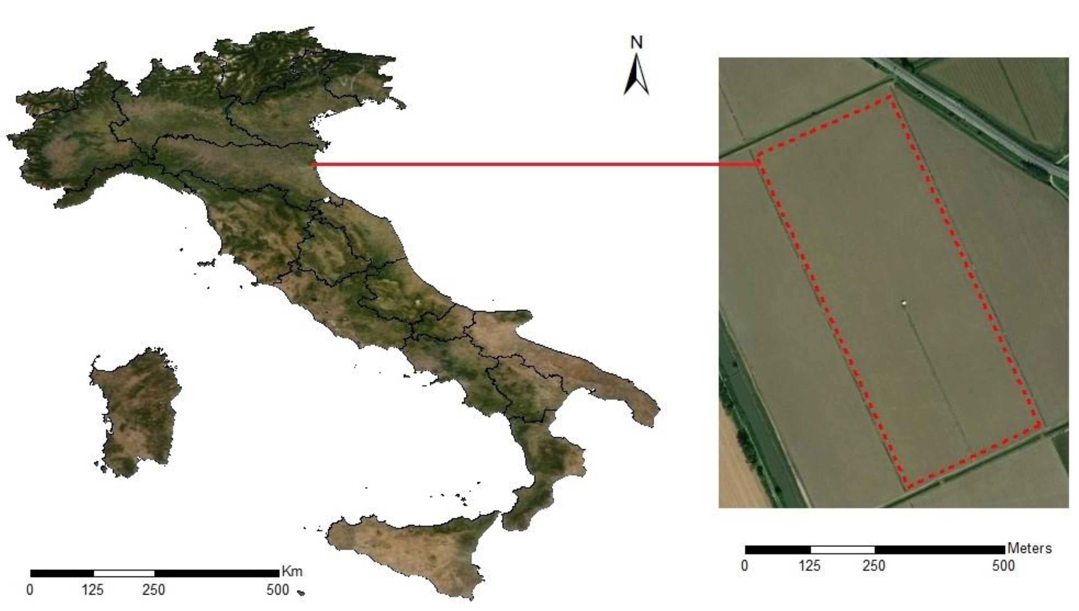
2.1. Study Area

This study was carried out on a 22-ha field located in a typical valley area (at Porto Felloni Co.) in Ferrara, North Italy (Figure 1). The study field lies within the Mediterranean climatic zone and the total rainfall during the corn growing season was 266 mm on average. The soil texture is silt loam and the study field has been irrigated by a center pivot irrigation system and cultivated with corn for two decades, with the exception of 2015, when it was cultivated with wheat. This work focused on three years of corn cultivation from 2016 to 2018. The corn planting dates were 30 March 2016, 22 March 2017 and 11 April 2018 for the study field and harvest was done at a crop age of 160 days on average. The company cultivated the same corn seed variety (Pioneer P1916) during the study period with 75 cm of row spaces and 16 cm between seeds, on average. Additionally, they used a variable rate of nitrogen application with an average urea application (nitrogen 46%) of 344 kg/ha in 2016 and 2017 and 367 kg/ha in 2018. The prescription map of applied nitrogen was the same for the 2016 and 2017 seasons and modified for the 2018 season.

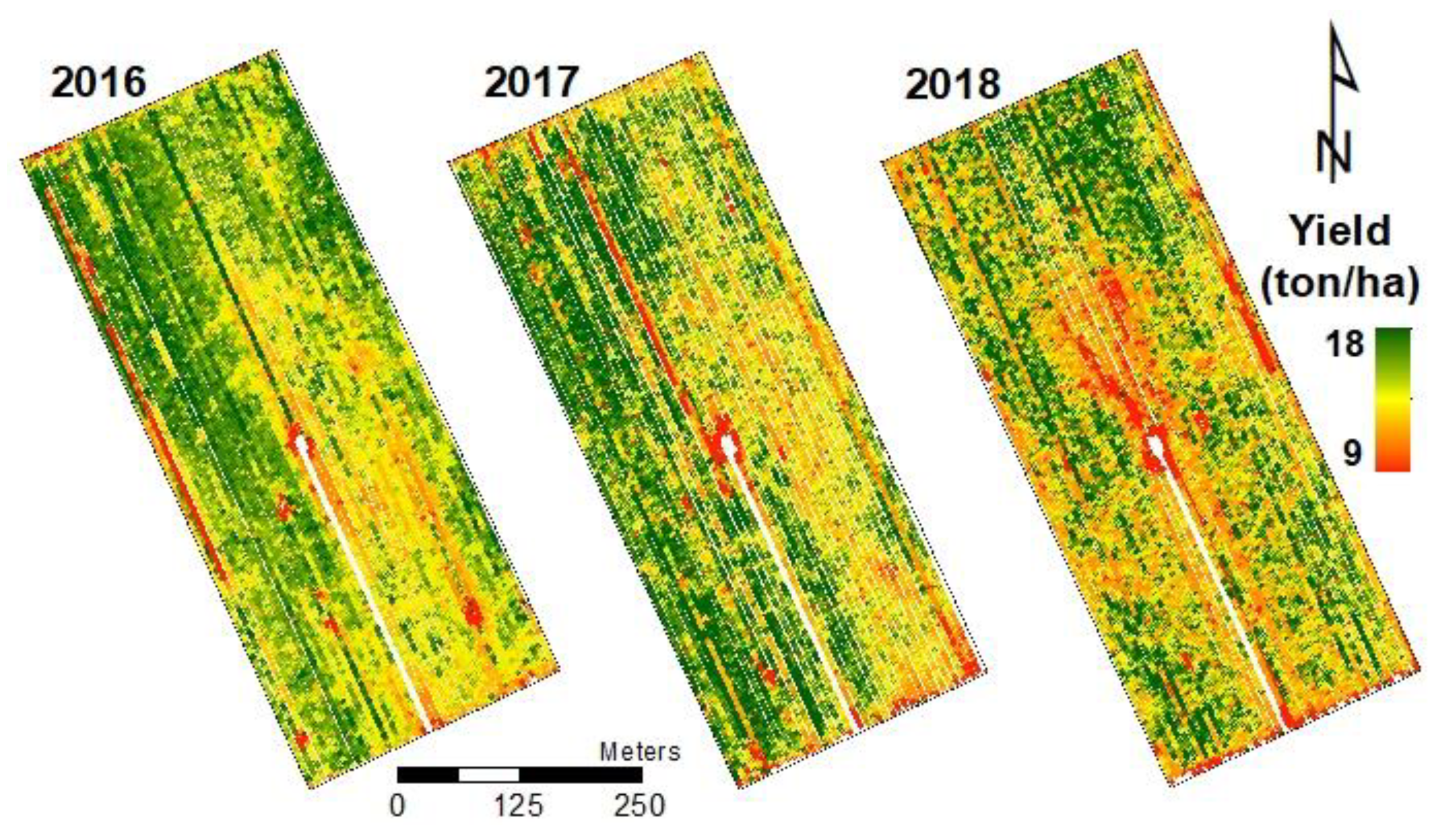
2.2. Measured Yield Data

A grain yield monitoring system mounted on a combine harvester was used to record corn yield. This system could record about 1000 yield points for each hectare (about 20,000 points from the whole study field). The harvester width was 6 m and the monitor could record yield every 1 s, which is equivalent to an average speed of the harvester of 1.5 m along the direction of harvesting. Corn yield varied between 9 and 18 ton/ha across the study field for the three seasons. After harvesting and downloading the yield data, maps were processed as follows. Field borders were removed to avoid noise arising from the partial presence of corn in the field margins. Data recorded while the harvesting machine was turning at the end of each line were also removed to avoid zero production from the corresponding field portions. Secondly, two lines were removed from the 2016 yield data where the harvester passed twice during field operations. The measured yield is provided as a dataset with ~20,000 sparse points, whereas the Sentinel-2 data is a raster with a 10-m resolution. Therefore, the sparse points were interpolated to a raster with the same resolution as Sentinel-2 using the Kriging method. Kriging was run using R’s Gstat package. The best models and fits (range, partial sill, and nugget) are, respectively, for each of the three seasons from 2016 to 2018: (i) Exponential—57.29 m, 1.628, 2.78; (ii) Exponential—46.18 m, 3.087, 5.123; (iii) Spherica—114.87 m, 3.982, 5.55. The field contains 2006 cells with yield values for each of the three seasons analyzed. Figure 2 shows a color-scaled image of the final corn yield data for the three studied seasons.

2.3. Satellite Imagery

Sentinel-2 Level 2A (L2A) Bottom-Of-Atmosphere (BOA) reflectance product was acquired from the Copernicus Open Access Hub. Sentinel-2 L2A data provided 12 bands with channels ranging from 443 to 2190 nm and a spatial resolution (ground sampling distance—GSD) of 10 to 60 m [54]. All images were resampled to 10 m pixel size and clipped to the region of interest (the study field).

To compare between the plant development stages, we used “crop age”, defined by the number of days counted from the planting date. The crop ages at harvesting time were 168, 159, and 160 days from planting for 2016, 2017, and 2018, respectively. In our case, there were no available cloud-free Sentinel-2 images until a crop age of 60 days (April and May). Starting from June, cloud-free satellite images were more frequently available. In 2016, there were only six Sentinel-2 images available. This number increased to reach 14 images per season for 2017 and 2018. A total of 34 Sentinel-2 images between 2016 and 2018 were available during the corn growing season at different crop ages, as shown in

Table 1. Sentinel-2 images dates corresponding crop age in days and phenological stage at each growing season.

2016 Season			2017 Season			2018 Season
Planting Date: 30 March 2016			Planting Date: 22 March 2017			Planting Date: 11 April 2018
Harvesting Date: 14 September 2016			Harvesting Date: 25 August 2017			Harvesting Date: 18 September 2018
I	Date	Age (Stage)	I	Date	Age (Stage)	I	Date	Age (Stage)
1	18 June 2016	80 (R3)	1	31 May 2017	70 (R2)	1	19 May 2018	38 (V10)
2	18 July 2016	110 (R4)	2	03 June 2017	73 (R2)	2	10 June 2018	60 (R1)
3	28 July 2016	120 (R5)	3	13 June 2017	83 (R3)	3	15 July 2018	95 (R3)
4	04 August 2016	127 (R6)	4	20 June 2017	90 (R3)	4	18 July 2018	98 (R4)
5	14 August 2016	137 (R6)	5	23 June 2017	93 (R3)	5	20 July 2018	100 (R4)
6	24 August 2016	147 (R6)	6	03 July 2017	103 (R4)	6	28 July 2018	108 (R4)
			7	10 July 2017	110 (R4)	7	04 August 2018	115 (R6)
			8	13 July 2017	113 (R5)	8	17 August 2018	128 (R6)
			9	23 July 2017	123 (R6)	9	19 August 2018	130 (R6)
			10	30 July 2017	130 (R6)	10	22 August 2018	133 (R6)
			11	02 August 2017	133 (R6)	11	24 August 2018	135 (R6)
			12	04 August 2017	135 (R6)	12	27 August 2018	138 (R6)
			13	12 August 2017	143 (R6)	13	29 August 2018	140 (R6)
			14	22 August 2017	153 (R6)	14	06 September 2018	148 (R6)

.

Clouds and other opaque aerosol in the atmosphere can partially occlude the transmission of energy at the wavelengths recorded by the Multispectral Instrument (MSI) on-board Sentinel-2. Level 2A products provide a raster map with cloud cover confidence ranging from 0 for high confidence of clear sky to 100 for high confidence of cloudy sky [54]. This information was used to isolate pixels with a cloud probability above zero. Out of 34 images, 14 had at least one pixel covered by clouds.

Table 2. Number of pixels covered by clouds in each image and cloudy sky confidence (%) of removed pixels.

		Cloudy Sky Confidence
Image Date	N. Pixels *	Min	Mean	Max
18 June 2016	6	1	1.83	2
18 July 2016	4	1	1.00	1
28 July 2016	4	1	1.00	1
24 August 2016	4	1	1.00	1
31 May 2017	70	1	1.17	3
3 June 2017	690	1	1.08	5
13 June2017	619	1	1.05	5
23 June 2017	4	2	2.00	2
10 July 2017	4	1	1.00	1
13 July 2017	4	4	4.00	4
2 August 2017	12	1	1.00	1
4 August 2017	4	1	1.00	1
12 August 2017	4	1	1.00	1
10 June 2018	4	3	3.00	3

* Number of pixels with cloudy sky confidence above zero. There are a total n. of 2006 pixels (10 m GSD) in the study area.

below gives an overview. The study crop field covered 2006 pixels at 10 m GSD. All pixels with cloud probability above zero were masked and thus not considered for further processing. Masking removed these pixels from further processing.

2.4. Vegetation Indices

Nine different vegetation indices (NDVI, NDRE1, NDRE2, GNDVI, GARVI, EVI, WDRVI, mWDRVI, and GCVI) were derived from Sentinel-2 images after resampling all bands to 10 m pixel size using SNAP software (Sentinel application platform) version 5.0. These indices are the most common VIs used for crop yield monitoring in the literature and were derived using Equations (1)–(9).

$$NDVI=\frac{\mathrm{NIR}-\mathrm{B}4}{\mathrm{NIR}+\mathrm{B}4},$$

(1)

$$NDRE1=\frac{\mathrm{NIR}-\mathrm{B}5}{\mathrm{NIR}+\mathrm{B}5},$$

(2)

$$NDRE2=\frac{\mathrm{NIR}-\mathrm{B}6}{\mathrm{NIR}+\mathrm{B}6},$$

(3)

$$GNDVI=\frac{\mathrm{NIR}-\mathrm{B}3}{\mathrm{NIR}+\mathrm{B}3},$$

(4)

$$GARVI=\frac{\mathrm{NIR}-\left(\mathrm{B}3-\mathrm{B}1-\mathrm{B}5\right)}{\mathrm{NIR}-\left(\mathrm{B}3+\mathrm{B}1-\mathrm{B}5\right)},$$

(5)

$$EVI=\frac{\mathrm{NIR}-\mathrm{B}4}{\mathrm{NIR}+6\mathrm{B}4-7.5\mathrm{B}1+1}\times 2.5,$$

(6)

$$WDRVI=\frac{\mathsf{\alpha }\times \mathrm{NIR}-\mathrm{B}4}{\mathsf{\alpha }\times \mathrm{NIR}+\mathrm{B}4},$$

(7)

$$mWDRVI=\{\begin{array}{lll}NDVI& & NDVI\le 0.6\\ WDRVI& & NDVI>0.6\end{array},$$

(8)

$$GCVI=\left(\frac{\mathrm{NIR}}{\mathrm{B}3}\right)-1,$$

(9)

where NDVI is the Normalized Difference Vegetation Index (Equation (1)), NDRE 1 and 2 are the Normalized Difference Red Edge calculated based on band numbers 5 and 6, respectively (Equations (2) and (3)), GARVI is the Green Atmospherically Resistant Vegetation Index (Equation (4)), GNDVI is the Green Normalized Difference Vegetation Index (Equation (5)), EVI is the Enhanced Vegetation Index (Equation (6)), WDRVI is the Wide Dynamic Range Vegetation Index (Equation (7)), and mWDRVI is a mixed WDRVI where the WDRVI value is used conditionally if the NDVI value is above 0.6, otherwise NDVI is used, as per the literature in [34,55] (Equation (8)). GCVI is the Green Chlorophyll Vegetation Index (Equation (9)). B1 is the reflectance of the blue band (432–453 nm), B3 is the reflectance of the green band (542–578 nm), B4 is the reflectance of the red band (649–680 nm), B5 and B6 are the reflectance of the vegetation red edge band at (697–712 nm) and (733–748 nm), respectively, and NIR is the reflectance of the near-infrared bands of the Sentinel-2 satellite images. For NIR, we tested bands 8, 8A, and 9, at (780–886 nm), (854–875 nm), and (935–955 nm), respectively, for all the VIs. The α value in WDRVI is a weighting factor equals to 0.15 as average value between 0.1 and 0.2 as it is reasonable according to literature [55]. The derived vegetation indices were analyzed and compared with the actual yield maps for each season. The correlation measured using R² value was calculated for each index at different crop ages.

2.5. Yield Prediction with Machine Learning

The prediction of a continuous variable, i.e., regression, can be done with several ML approaches. Three algorithms were tested in this investigation: multiple regression (MR), random forests (RF), and support vector machines (SVM). The last two are nonparametric methods, as the number of parameters in the model is not fixed, but changes depend on the data used for training—which usually grows as the training data volume increases [46]. These models were chosen because in the existing literature, they have been proven to yield better results when compared with other methods [56,57,58,59,60]. The independent variables were the reflectance values of the considered bands and the dependent variable to be predicted was the yield value. At each image, band values were used as independent variables to train a model using the values in the raster derived from the measured yield, as described in Section 2.2.

Multiple regression uses multiple simple linear regressions on the input variables using least squares optimization to define the best fit for each dependent variable as a function of the independent variable (measured yield). This is the simplest model and assumes a linear relationship between the yield and the band reflectance values, and that band values are not correlated. This last assumption is known to be untrue, as band values are correlated; thus, this method was applied to the first four principal components which contained 92% of variance.

Random Forests (RF) is a method based on decision trees for classification and regression. The training data are used to define decision boundaries that create the “trees” in the “forest” via split nodes in the decision tree process. The best combinations of splits are defined by a bootstrap approach. The available training data is sampled without replacement, keeping the remaining data for determining residuals from an independent set (out-of-bag validation) and thus comparing the accuracy metrics between combinations and choosing the best. Two main parameters need to be defined by the user: the number of features randomly sampled as candidates at each split—usually the square root of the total number of features—and the number of trees to grow.

The Support Vector Machine (SVM) method defines boundaries in high-dimensional space, i.e., a hyperplane, that separates training data into labelled classes, which, in our case, is a continuous variable (yield) for the regression task. Nonlinear boundaries use a nonlinear kernel function, in our case, the Radial Basis kernel “Gaussian” RBF. For more information on the method, there is extensive literature on SVM applied to remote sensing [45,48,56,57].

In order to validate the tested models, the predicted yield was compared against the measured yield from independent samples. Only cells that were free from clouds were used by masking any cell with a cloud coverage probability above zero (see Table 2). The cause for using this conservative threshold is to avoid the noise from clouds taking into consideration that this study investigated the within-field variability of a relatively small area cultivated with the same crop through limited satellite spectral reflectance bands. Therefore, for each cloud-free date, we made 2006 observations with 12 variables, i.e., reflectance values of the land cover at the time the satellite image was recorded. In case of clouds, fewer cells were used.

The model was run 60 times, each time randomly dividing data into two parts and using one half for training and the remaining half for validation. This procedure was repeated to assess variation in accuracy metrics when using different point samples for training. Five accuracy metrics were extracted in order to obtain a thorough overview of the distribution of errors as per Equations (10)–(14).

$$ME=\frac{{\sum }_{i=1}^n{y}_i-x_i}{\mathrm{n}},$$

(10)

$$MAE=\frac{{\sum }_{i=1}^n\left|y_i-x_i\right|}{\mathrm{n}},$$

(11)

$$MAPE=\frac{{\sum }_{i=1}^n\left|\frac{y_i-x_i}{y_i}\right|\times 100}{\mathrm{n}},$$

(12)

$$RMSE=\sqrt{\frac{{\sum }_{i=1}^n{\left(y_i-x_i\right)}^2}{n}},$$

(13)

$$R^2=1-\frac{{\sum }_{i=1}^n{\left(y_i-x_i\right)}^2}{{\sum }_{i=1}^n{\left(y_i-\overline{y}\right)}^2},$$

(14)

where MAE is the mean absolute errors, MAPE is the mean absolute percentage error, ME is the mean error, R² is the R-squared, RMSE is the root mean square of errors, x is the measured yield value, y is the predicted yield value, n is the number of observations, i is the iteration of observations, and $\overline{y}$ is the mean value of predicted yield. All procedures were carried out in R with an rminer package [61,62]. The results show that random forests [63] provided the most accurate results. Therefore, random forests was used for further tuning and analysis (see Results section).

3. Results

The following sections report on results from VIs and machine learning approaches. Correlations of VIs with yield were analyzed to assess how VIs can potentially be used to model yield. The three machine learning models were assessed with the five mentioned accuracy metrics.

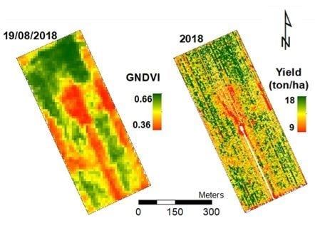
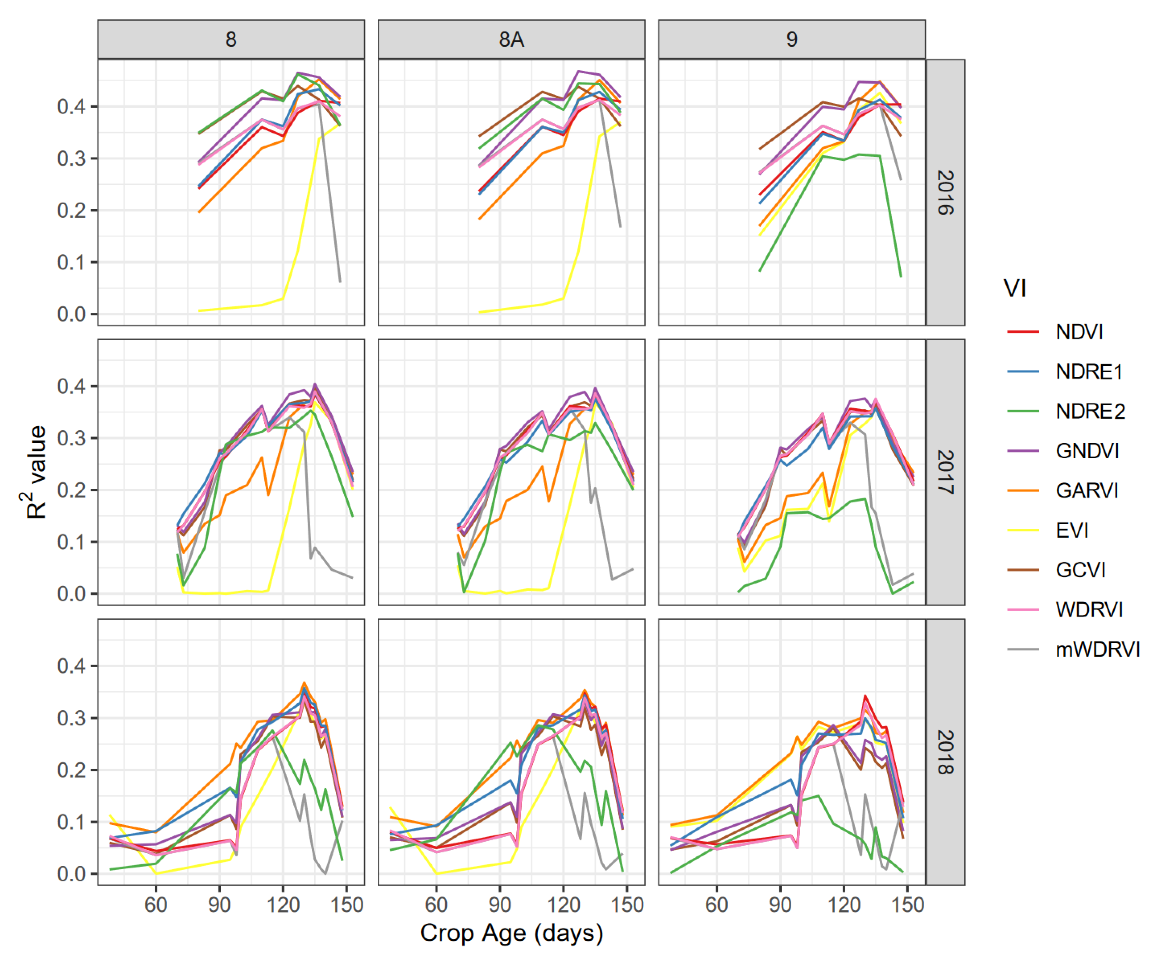
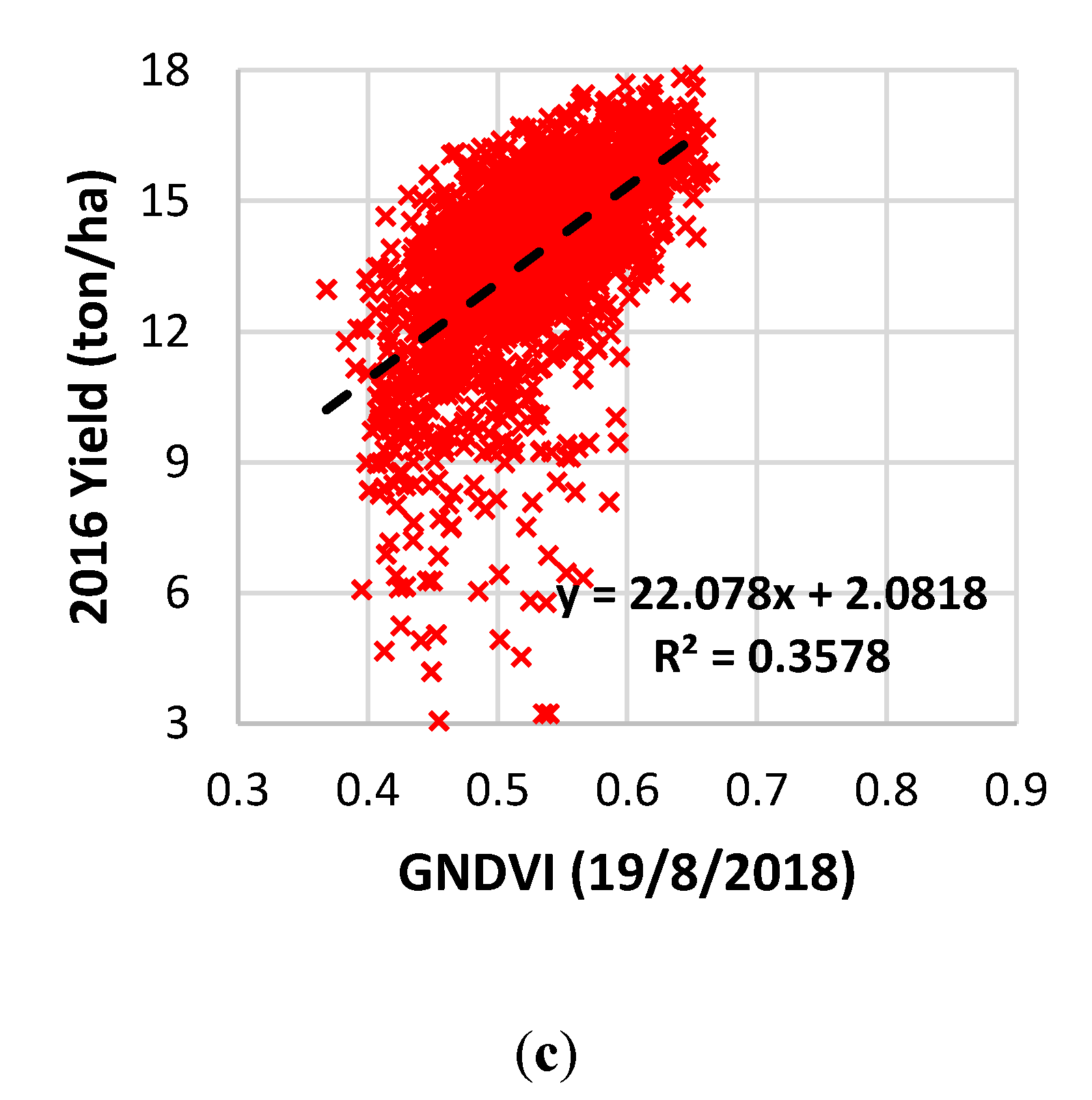
3.1. Vegetation Indices

Each year presented a different pattern of yield spatial distribution due to different soil characteristics, variable rate nitrogen application by the farmer, and other weather conditions. In general, the yield maps showed a high yield at the north-western zone of the field compared with the south-eastern zone in 2016 and 2017 (Figure 2). In 2018, yield improved in the south-eastern zone while yield decreased in the north-western zone compared to previous seasons.

Nine vegetation indices (NDVI, NDRE1, NDRE2, GNDVI, GARVI, EVI, WDRVI, mWDRVI, and GCVI) derived from each Sentinel-2 image calculated with three different NIR bands (8, 8A, and 9) were correlated with the actual yield map of each year. In general, correlations based on bands 8 and 8A were higher than those based on band 9. Band 8 and 8A correlations had the same trend for all seasons and at all crop ages with slight differences. Band 9 has a spatial resolution of 60 m which provided only 57 pixels for the whole study field compared to band 8A and 8, which have a spatial resolution of 20 and 10 m and provided 516 and 2067 pixels, respectively. The higher spatial resolution could describe the field variability more accurately and improve the correlation results. Therefore, VIs based on band 8 were considered for further analysis.

The correlation between vegetation indices and corn grain yield (Figure 3) were low at the vegetative growth stages and early reproductive development stages (first 80 days of crop age) for 2017 and 2018 seasons. This correlation increased during the grain filling stage R3 (90 to 110 days) and reached its peak at the physiological maturity stage R4–R6 (105 to 135 days). This trend could be realized from the three seasons correlations (R² value), as shown in Figure 3. In 2016, the coefficient of determination (R² value) started from less than 0.2 at a crop age of 80 days (R3) and reached the highest R² value of 0.48 at 137 days (R6) from GNDVI. In 2017, a clearer trend was observed due to the higher number of available images, starting from an R² value of less than 0.2 at a crop age of 70 days (R2) and more than 0.35 for five different images from a crop age of 110 to 135 days (R4–R6). The highest R² value was for GNDVI compared to the other investigated indices at all stages, which reached a peak of 0.42 at the R6 stage at a crop age of 135 days. In 2018, R² values were not stable due to fog and blur in the images that affected the image quality but followed the same trend as previous seasons. The R² values started from less than 0.1 at a crop age between 60 and 100 days (R1–R4), then improved to reach the peak of 0.37 from GARVI and 0.36 from GNDVI at a crop age of 130 days (R6). All correlations between VIs and corn grain yield for all satellite image dates are available in the Supplementary files.

GARVI provided the highest correlations in 2018 slightly higher than GNDVI. GARVI is more resistant to atmospheric effects, as described by Gitelson et al. [30], which explain GARVI’s trend for this season in particular. Moreover, the correlation decreased dramatically at a crop age of 140 days for the 2017 and 2018 seasons with a R² value of less than 0.25, while it decreased to 0.4 for 2016. After 140 days, the crop enters the stage of full maturity and leaves turns from green to brown, thus decreasing the coefficient of determination R² value. The highest R² value was observed from GNDVI at crop ages of 127, 135, and 130 days for 2016, 2017, and 2018, respectively. The corn yield maps after kriging and resampling to a 10 m pixel size with mostly correlated GNDVI and corresponding R² graph are shown in Figure 4. In Figure 4, GNDVI and yield maps are shown with the same color map stretched with the histogram equalization method.

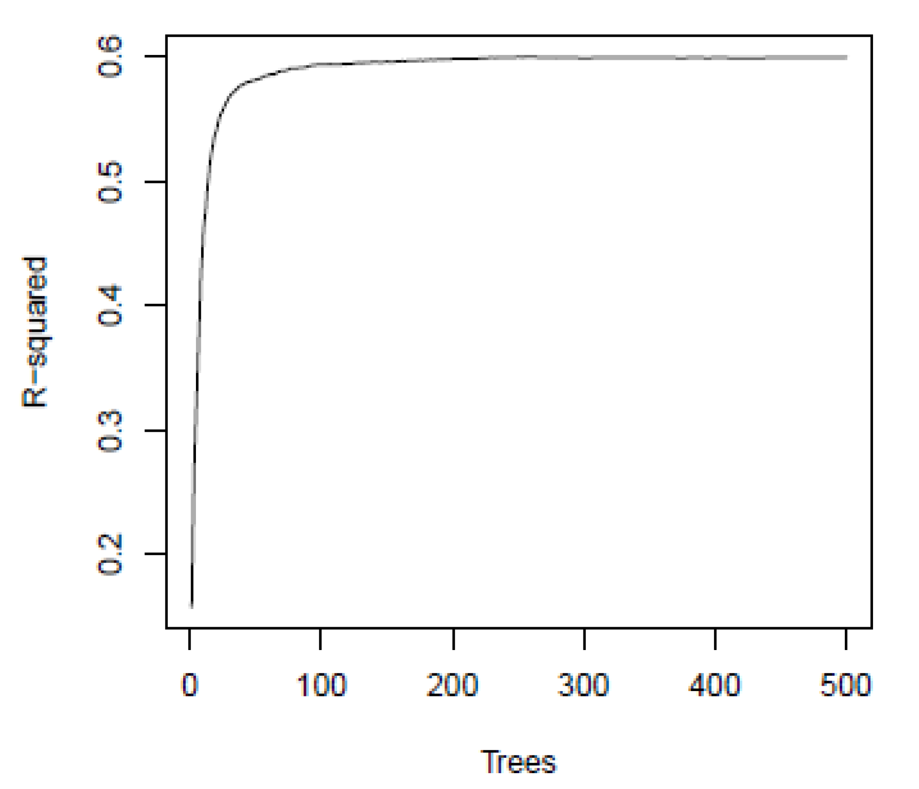
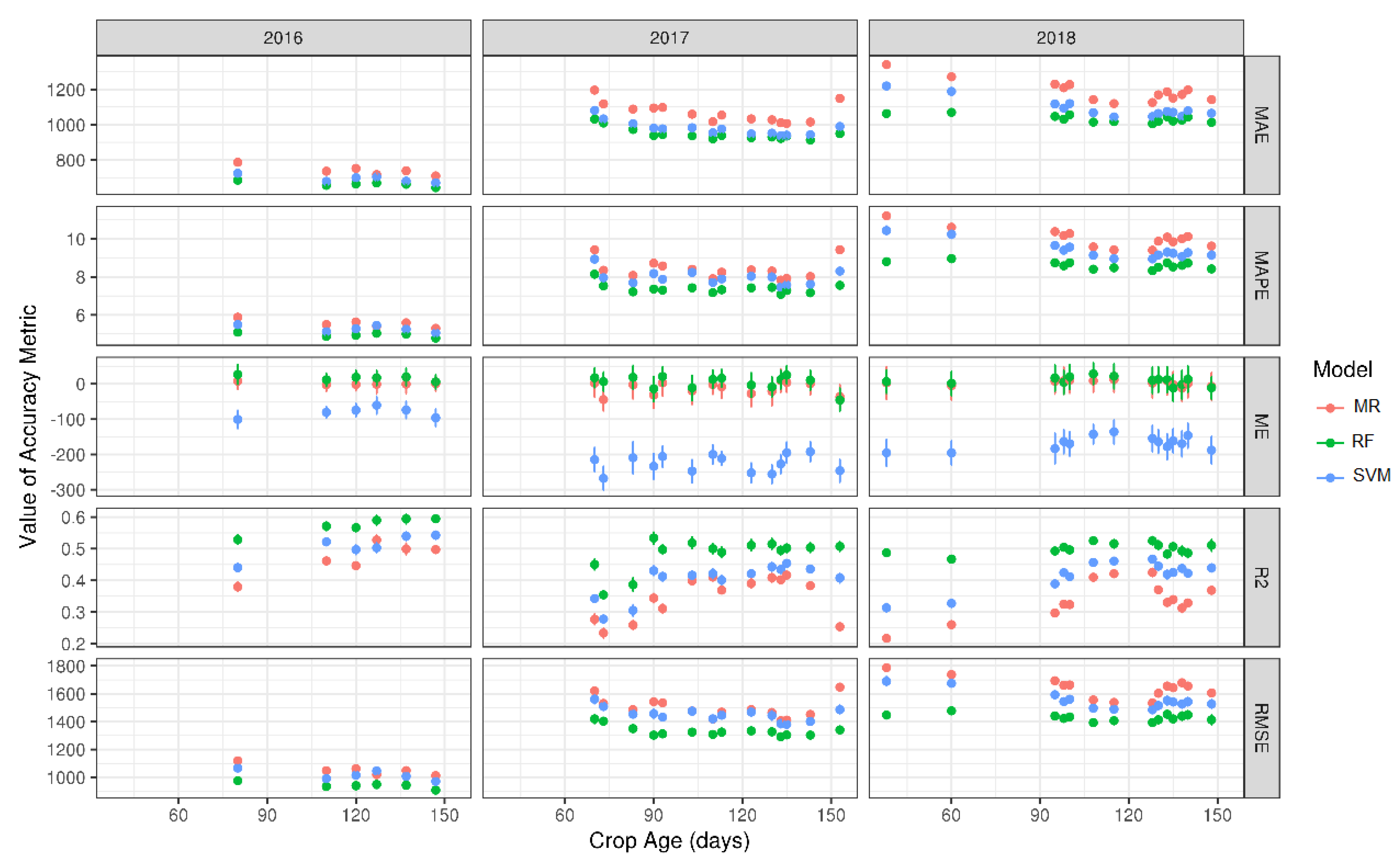
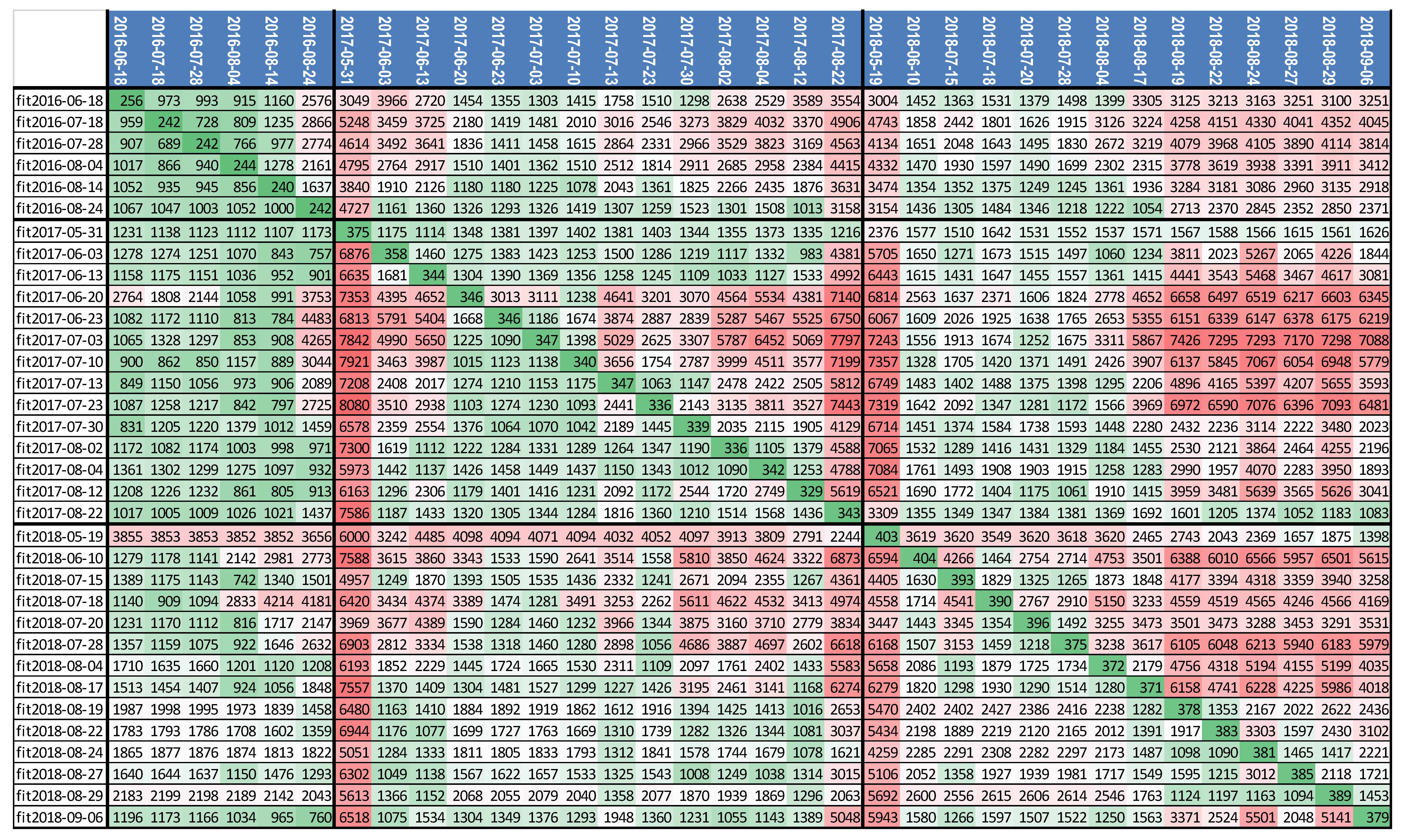
3.2. Machine Learning Models

The random forests algorithm can be tuned by changing two parameters: the number of trees (Nt) and the number of features (Nf). Iterative methods to find the best Nt and Nf combinations were applied by testing 3 × 5 combinations of Nf $\in$ {4, 8, 12} and Nt $\in$ {50, 100, 120, 200, 500}. The best combination resulted in Nf = 4 and Nt = 120. Each node in a tree is split by randomly selecting Nf features from the d-dimensional input feature space. Figure 5 shows how accuracy grows by increasing the number of trees, with the optimal value when no significant increase is seen. Figure 6 and Figure 7 show that the results were optimal at a certain time from planting the crops, which is in line with results from vegetation indices correlations but with a higher overall R² value.

The Random Forests method gave more accurate results when compared with other types of models that use decision trees and neural network ensembles (Figure 6). For each training and validation step, more runs were carried out, as mentioned in the Methods section; therefore, variance can be reported and is visible in the plot as standard deviation whiskers (Figure 6). Only ME had a high enough value of standard deviation to be visible in the plot, showing that the absolute accuracy metrics are significantly different between methods. This is coherent with the existing literature [56,57].

Figure 6 shows the result of the five calculated accuracy metrics, as reported in Equations (10)–(14). The mean absolute error (MAE) and the same as a percentage (MAPE) can distinguish how the best ML method ranges between 0.7 and 1.0 ton/ha, which corresponds to 5–8% of measured yields. Mean error is useful to assess bias; support vector machines ME values show that predicted yield values underestimated with respect to measured values. The whiskers in Figure 6 in the plot of the mean error show the variation of bias of each model when predictions were compared with measured yield values. This variation is +/− 0.05 ton/ha, which is minimal considering the 9 to 18 ton/ha range within-field zones. The correlation coefficient is reported for comparison reasons against the correlations found using the VIs reported in the previous section. Root mean square of errors is an important metric that is more sensitive than MAE to residuals of predicted and measured yield values.

The results in Figure 7 report the accuracy of each model trained using certain images at certain dates (rows) when predicting yield values using other images from other dates (columns). More is discussed on this in the next section. The most accurate results (low MAE values) were provided by the 2016 images compared to 2017 and 2018. The availability of more images in 2017 and 2018 showed that MAE values are higher during the early and late corn growing stages which is in line with high correlations in R4–R6 growing stages.

4. Discussion

The first outcome of this study is that GNDVI showed the highest correlation between VI and corn grain yield. This result is in line with Shanahan et al. [41], who reported the same index from aircraft imagery at a small scale. In addition, Schwalbert et al. [19] and Peralta et al. [18] reported that GNDVI and NDVI reflected the potential on corn yield prediction models. The difference between the examined VIs was not large, except for EVI, but GNDVI showed a clearer trend and the highest correlations. This result is clearer in the 2017 season, while other seasons have more fluctuation in other VIs and less image availability. Gitelson et al. [30] reported that GNDVI is more sensitive to the chlorophyll concentration in a wide range of chlorophyll variations. Additionally, they reported that the reflectance range between 520 and 630 nm is the most sensitive for chlorophyll. This range matches with the green band B3 of Sentinel-2 data that ranges between 524 and 596 nm. Meanwhile, Tan et al. [64] reported that GNDVI was the most positively correlated vegetation index with FPAR for corn canopies which subsequently describes the strong relation to corn biomass and yield.

Secondly, GNDVI derived from Sentinel-2 images in the study field could provide a clear description of the corn grain yield spatial variability within-field scale for around 1 month between the end of grain filling and physiological maturity stages. This period is around the physiological maturity stages (R4–R6) at crop ages of 105 to 135 days from planting and mostly between mid-July and mid-August in North Italy. This period was mentioned by Ferencz et al. [42] in a Hungarian county scale, Shanahan et al. [41], and Maestrini and Basso [40] in the USA for corn yield prediction. The consistency for this period in the USA, Hungary, and Italy and with multiple scales supports defining it as the most suitable corn yield prediction time. This period is the summer season with less probability of clouds and fog, and Sentinel-2 could provide about six images during this month, which could describe the corn grain yield variability within-field.

Machine learning provides overall higher R² and more robust results than the VIs approach. Practical results from this study are clearly the application of random forests after 105 days from planting, training the model with a few ground truths sampled over the field, and then applying the trained model over other fields that must be modelled. Evidently, fields must have similar characteristics. The final target is to have a mapped spatial distribution of corn yield over the field of interest that could support farmers for site specific applications.

Another result pertaining to the application of machine learning models with Sentinel-2 reflectance timeseries data for crop yield prediction is depicted in Figure 7. Figure 7 reports on the accuracy of a model that was fitted by training with imagery from a certain date (rows), applied to imagery from all other dates (columns). The diagonal row in this table represents fitting and modelling on the same image and, as expected, provided the best performance. Other combinations show how well a model that is fitted on one image date performs on another image date. Figure 7 shows that the model must be used in the same conditions of crop growing stage to replicate acceptable accuracies. Machine learning methods are nonparametric methods and have many advantages, as mentioned here and in other studies, but are not easily interpreted and, therefore, replication of a model with imagery from other dates or different conditions is not advised.

Another aspect worth discussing is that correlations became worse from 2016 to 2018 for VIs. In machine learning, it is clear that compared to other models, 2016 provided the highest coefficients of determination (Figure 6 and Figure 7). In Figure 7, the 2016 images (columns) provided better accuracy values with other models (rows) than other years, in particular, in August, as the columns show lower MAE values. There are possible explanations for 2016 being a better year for predicting yield values that can be brought forward, even if at this stage, they are only hypotheses. One important point to consider is the accuracy of the measured yield values. The measured yield values are used as “truth”, but as all measures go, they are prone to a certain degree of error. The method used for measuring provides about 10 times higher accuracy than prediction models, but it can record values incorrectly, such as explained in the materials section, i.e., border effects, harvester passing twice. Then, it might be possible that seasons 2017 and 2018 yield data underwent higher errors due to unpredicted or unseen sensor or measurement distortions such as GPS and yield sensors’ inaccuracies or calibration errors from year to year. This can explain the overall difference in correlation and prediction accuracy between years, as the measured yield is fixed per year. Burke and Lobell [35] have found R² up to 0.4 for corn yield prediction from RS data, stressing the importance of the quality of the field measures. Another possible and probably more realistic hypothesis can be related to atmospheric conditions, as the images in 2017 and 2018 might have suffered from more opaque atmospheric conditions, not so much to be detected as cloud probability by the sen2cor algorithm used in Sentinel-2 processing.

Even the relation between yield and VIs are affected by spatial and temporal constraints, as reported by many researchers [19], but it could be used for identifying management zones [7,65], evaluating within-field variability and subsequently, the need for PA practices. According to the study results, Sentinel-2 could assess only 40–60% of field variability: such percentage is clearly unsatisfactory if seen at single pixel level, but is fully acceptable in common PA practices, where management zones are to be defined. Indeed, in this case, a relatively high number of values are averaged within each MZ (typically larger than 1 acre, corresponding to at least 40 pixels) eventually allowing reduction of variability and a corresponding increase of overall robustness of the method. Within-field variability is common due to variations in soil type, topography, nutrient level, and many other factors of agricultural fields. Mapping this variability, delineating to homogeneous zones, and applying the variable rate application of agricultural inputs leads to more profitable and efficient management practices. In addition, the archived Sentinel-2 images could provide an important source for monitoring fields’ history and the cumulative production for each zone. Recent studies reported that the profit of PA applications ranged between −30 $/ha and 70 $/ha and about 25% of studies reported economic losses [66]. In view of this, evaluating field spatial variability on previous seasons from archived satellite images could be a simple approach to evaluate the actual need for site-specific management practices. Mulla [67] highlighted the necessity of integrating archived satellite images for PA decision support systems and this approach could be a promising application in this field. Moreover, monitoring yield variability within fields through archived satellite images could be applied for different crops, varieties, countries, and farming management practices to widen the use of archived data.

5. Conclusions

A field study was conducted to investigate the possibility of monitoring corn grain yield within a 22-ha field using Sentinel-2 satellite images. Actual corn yield maps for three seasons were correlated with different vegetation indices and crop ages through the implementation of machine learning techniques. Monitoring the within-field variability of corn yield was possible and the R² value reached more than 0.5 in some cases. The main findings can be summarized as follows:

-

GNDVI was the most correlated VI with corn grain yield at the field scale;

-

the most suitable time for corn yield forecasting was during the physiological maturity stages (R4–R6) between 105 and 135 days from the planting date, i.e., between mid-July and mid-August;

-

this period is not only the most correlated, but also is provides a higher number of satellite images due to reduced cloud events in the area considered;

-

Random Forests was the most accurate machine learning technique in corn yield monitoring with R² values almost reaching 0.6 in an independent validation set;

-

the Random Forests method works best when trained with imagery close to the above-mentioned most suitable time for forecasting; applying it to images at different crop stages is not advised.

The overall question “can Sentinel-2 imagery be used to predict corn yield values?” can be answered by saying that in a scenario with expected yields between 9 and 18 ton/ha, a likely prediction with a 10% error can be expected using a Random Forests model trained with a few ground samples taken between 105 and 135 days of crop age. Without ground samples of yield values, thus, with less effort on the ground, one can validly use GNDVI at the same crop age range for understanding the spatial variation of yield. Future research will use more tests to understand the ideal combination of volume of training data and the spatial distribution of training data for understanding the best economical combination for an accurate prediction of corn yield with the least effort in terms of surveying training data for the model.

References

1. Ross, K.W.; Morris, D.K.; Johannsen, C.J. A Review of Intra-Field Yield Estimation from Yield Monitor Data. Appl. Eng. Agric. 2008, 24, 309–317. [Google Scholar] [CrossRef]
2. Trotter, T.F.; Fraizer, P.S.; Mark, G.T.; David, W.L. Objective Biomass Assessment Using an Active Plant Sensor (Crop circletm)—Preliminary Experiences on a Variety of Agricultural Landscapes. In Proceedings of the 9th International Conference on Precision Agriculture (ICPA), Denver, CO, USA, 20–23 July 2008. [Google Scholar]
3. Pezzuolo, A.; Basso, B.; Marinello, F.; Sartori, L. Using SALUS model for medium and long term simulations of energy efficiency in different tillage systems. Appl. Math. Sci. 2014, 8, 6433–6445. [Google Scholar] [CrossRef]
4. Al-Gaadi, K.A.; Hassaballa, A.A.; Tola, E.; Kayad, A.; Madugundu, R.; Assiri, F.; Alblewi, B. Characterization of the spatial variability of surface topography and moisture content and its influence on potato crop yield. Int. J. Remote Sens. 2018, 39, 8572–8590. [Google Scholar] [CrossRef]
5. Lobell, D.B.; Thau, D.; Seifert, C.; Engle, E.; Little, B. A scalable satellite-based crop yield mapper. Remote Sens. Environ. 2015, 164, 324–333. [Google Scholar] [CrossRef]
6. Kross, A.; McNairn, H.; Lapen, D.; Sunohara, M.; Champagne, C. Assessment of RapidEye vegetation indices for estimation of leaf area index and biomass in corn and soybean crops. Int. J. Appl. Earth Obs. Geoinf. 2015, 34, 235–248. [Google Scholar] [CrossRef] [Green Version]
7. Blackmore, S. The Role of Yield Maps in Precision Farming. Ph.D. Thesis, Cranfiled University at Silsoe, Cranfiled, UK, 2003. [Google Scholar]
8. Bouman, B.M. Crop modelling and remote sensing for yield prediction. Neth. J. Agric. Sci. 1995, 43, 143–161. [Google Scholar]
9. Yao, F.; Tang, Y.; Wang, P.; Zhang, J. Estimation of maize yield by using a process-based model and remote sensing data in the Northeast China Plain. Phys. Chem. Earth 2015, 87–88, 142–152. [Google Scholar] [CrossRef]
10. Huang, Y.; Zhu, Y.; Li, W.; Cao, W.; Tian, Y. Assimilating Remotely Sensed Information with the WheatGrow Model Based on the Ensemble Square Root Filter forImproving Regional Wheat Yield Forecasts. Plant Prod. Sci. 2013, 16, 352–364. [Google Scholar] [CrossRef] [Green Version]
11. Morel, J.; Todoroff, P.; Bégué, A.; Bury, A.; Martiné, J.F.; Petit, M. Toward a satellite-based system of sugarcane yield estimation and forecasting in smallholder farming conditions: A case study on reunion island. Remote Sens. 2014, 6, 6620–6635. [Google Scholar] [CrossRef] [Green Version]
12. Bala, S.K.; Islam, A.S. Correlation between potato yield and MODIS-derived vegetation indices. Int. J. Remote Sens. 2009, 30, 2491–2507. [Google Scholar] [CrossRef]
13. Mkhabela, M.S.; Bullock, P.; Raj, S.; Wang, S.; Yang, Y. Crop yield forecasting on the Canadian Prairies using MODIS NDVI data. Agric. For. Meteorol. 2011, 151, 385–393. [Google Scholar] [CrossRef]
14. Gao, F.; Anderson, M.; Daughtry, C.; Johnson, D. Assessing the variability of corn and soybean yields in central Iowa using high spatiotemporal resolution multi-satellite imagery. Remote Sens. 2018, 10, 1489. [Google Scholar] [CrossRef] [Green Version]
15. Lobell, D.B.; Ortiz-Monasterio, J.I.; Asner, G.P.; Naylor, R.L.; Falcon, W.P. Combining field surveys, remote sensing, and regression trees to understand yield variations in an irrigated wheat landscape. Agron. J. 2005, 97, 241–249. [Google Scholar]
16. Kayad, A.G.; Al-Gaadi, K.A.; Tola, E.; Madugundu, R.; Zeyada, A.M.; Kalaitzidis, C. Assessing the spatial variability of alfalfa yield using satellite imagery and ground-based data. PLoS ONE 2016, 11, e0157166. [Google Scholar] [CrossRef]
17. Al-Gaadi, K.A.; Hassaballa, A.A.; Tola, E.; Kayad, A.; Madugundu, R.; Alblewi, B.; Assiri, F. Prediction of potato crop yield using precision agriculture techniques. PLoS ONE 2016, 11, e0162219. [Google Scholar] [CrossRef]
18. Peralta, N.R.; Assefa, Y.; Du, J.; Barden, C.J.; Ciampitti, I.A. Mid-season high-resolution satellite imagery for forecasting site-specific corn yield. Remote Sens. 2016, 8, 848. [Google Scholar] [CrossRef] [Green Version]
19. Schwalbert, R.A.; Amado, T.J.C.; Nieto, L.; Varela, S.; Corassa, G.M.; Horbe, T.A.N.; Rice, C.W.; Peralta, N.R.; Ciampitti, I.A. Forecasting maize yield at field scale based on high-resolution satellite imagery. Biosyst. Eng. 2018, 171, 179–192. [Google Scholar] [CrossRef]
20. Asrar, G.; Kanemasu, E.T.; Yoshida, M. Estimates of leaf area index from spectral reflectance of wheat under different cultural practices and solar angle. Remote Sens. Environ. 1985, 17, 1–11. [Google Scholar] [CrossRef]
21. Patel, N.K.; Patnaik, C.; Dutta, S.; Shekh, A.M.; Dave, A.J. Study of crop growth parameters using Airborne Imaging Spectrometer data. Int. J. Remote Sens. 2001, 22, 2401–2411. [Google Scholar] [CrossRef]
22. Tucker, C.J.; Holben, B.N.; Elgin, J.H.; McMurtrey, J.E. Remote sensing of total dry-matter accumulation in winter wheat. Remote Sens. Environ. 1981, 11, 171–189. [Google Scholar] [CrossRef] [Green Version]
23. Ferencz, C.; Bognár, P.; Lichtenberger, J.; Hamar, D.; Tarcsai, G.; Timár, G.; Molnár, G.; Pásztor, S.; Steinbach, P.; Székely, B.; et al. Crop yield estimation by satellite remote sensing. Int. J. Remote Sens. 2004, 25, 4113–4149. [Google Scholar] [CrossRef]
24. Sibley, A.M.; Grassini, P.; Thomas, N.E.; Cassman, K.G.; Lobell, D.B. Testing remote sensing approaches for assessing yield variability among maize fields. Agron. J. 2014, 106, 24–32. [Google Scholar] [CrossRef]
25. Dubbini, M.; Pezzuolo, A.; De Giglio, M.; Gattelli, M.; Curzio, L.; Covi, D.; Yezekyan, T.; Marinello, F. Last generation instrument for agriculture multispectral data collection. Agric. Eng. Int. CIGR J. 2017, 19, 87–93. [Google Scholar]
26. Báez-González, A.D.; Chen, P.; Tiscareño-López, M.; Srinivasan, R. Using Satellite and Field Data with Crop Growth Modeling to Monitor and Estimate Corn Yield in Mexico. Crop Sci. 2002, 42, 1943–1949. [Google Scholar] [CrossRef]
27. Lobell, D.B. The use of satellite data for crop yield gap analysis. Field Crop. Res. 2013, 143, 56–64. [Google Scholar] [CrossRef] [Green Version]
28. Tucker, C.J. Red and photographic infrared linear combinations for monitoring vegetation. Remote Sens. Environ. 1979, 8, 127–150. [Google Scholar] [CrossRef] [Green Version]
29. Huete, A.R. A soil-adjusted vegetation index (SAVI). Remote Sens. Environ. 1988, 25, 295–309. [Google Scholar] [CrossRef]
30. Gitelson, A.A.; Kaufman, Y.J.; Merzlyak, M.N. Use of a green channel in remote sensing of global vegetation from EOS- MODIS. Remote Sens. Environ. 1996, 58, 289–298. [Google Scholar] [CrossRef]
31. Panda, S.S.; Ames, D.P.; Panigrahi, S. Application of vegetation indices for agricultural crop yield prediction using neural network techniques. Remote Sens. 2010, 2, 673–696. [Google Scholar] [CrossRef] [Green Version]
32. Xue, J.; Su, B. Significant Remote Sensing Vegetation Indices: A Review of Developments and Applications. J. Sensors 2017, 2017, 1–17. [Google Scholar] [CrossRef] [Green Version]
33. Sakamoto, T.; Gitelson, A.A.; Wardlow, B.D.; Verma, S.B.; Suyker, A.E. Estimating daily gross primary production of maize based only on MODIS WDRVI and shortwave radiation data. Remote Sens. Environ. 2011, 115, 3091–3101. [Google Scholar] [CrossRef]
34. Sakamoto, T.; Gitelson, A.A.; Arkebauer, T.J. MODIS-based corn grain yield estimation model incorporating crop phenology information. Remote Sens. Environ. 2013, 131, 215–231. [Google Scholar] [CrossRef]
35. Burke, M.; Lobell, D.B. Satellite-based assessment of yield variation and its determinants in smallholder African systems. Proc. Natl. Acad. Sci. USA 2017, 114, 2189–2194. [Google Scholar] [CrossRef] [PubMed] [Green Version]
36. Bu, H.; Sharma, L.K.; Denton, A.; Franzen, D.W. Comparison of satellite imagery and ground-based active optical sensors as yield predictors in sugar beet, spring wheat, corn, and sunflower. Agron. J. 2017, 109, 299–308. [Google Scholar] [CrossRef] [Green Version]
37. Liao, C.; Wang, J.; Dong, T.; Shang, J.; Liu, J.; Song, Y. Using spatio-temporal fusion of Landsat-8 and MODIS data to derive phenology, biomass and yield estimates for corn and soybean. Sci. Total Environ. 2019, 650, 1707–1721. [Google Scholar] [CrossRef]
38. Fieuzal, R.; Marais Sicre, C.; Baup, F. Estimation of corn yield using multi-temporal optical and radar satellite data and artificial neural networks. Int. J. Appl. Earth Obs. Geoinf. 2016, 57, 14–23. [Google Scholar] [CrossRef]
39. Rojas, O. Operational maize yield model development and validation based on remote sensing and agro-meteorological data in Kenya. Int. J. Remote Sens. 2007, 28, 3775–3793. [Google Scholar] [CrossRef] [Green Version]
40. Maestrini, B.; Basso, B. Predicting spatial patterns of within-field crop yield variability. F. Crop. Res. 2018, 219, 106–112. [Google Scholar] [CrossRef]
41. Shanahan, J.F.; Schepers, J.S.; Francis, D.D.; Varvel, G.E.; Wilhelm, W.W.; Tringe, J.M.; Schlemmer, M.R.; Major, D.J. Use of remote-sensing imagery to estimate corn grain yield. Agron. J. 2001, 93, 583–589. [Google Scholar] [CrossRef] [Green Version]
42. Bognár, P.; Ferencz, C.; Pásztor, S.Z.; Molnár, G.; Timár, G.; Hamar, D.; Lichtenberger, J.; Székely, B.; Steinbach, P.; Ferencz, O.E. Yield forecasting for wheat and corn in Hungary by satellite remote sensing. Int. J. Remote Sens. 2011, 32, 4759–4767. [Google Scholar] [CrossRef]
43. Rahman, M.M.; Robson, A.; Bristow, M. Exploring the potential of high resolution worldview-3 Imagery for estimating yield of mango. Remote Sens. 2018, 10, 1866. [Google Scholar] [CrossRef] [Green Version]
44. Mas, J.F.; Flores, J.J. The application of artificial neural networks to the analysis of remotely sensed data. Int. J. Remote Sens. 2008, 29, 617–663. [Google Scholar] [CrossRef]
45. Yuan, H.; Yang, G.; Li, C.; Wang, Y.; Liu, J.; Yu, H.; Feng, H.; Xu, B.; Zhao, X.; Yang, X. Retrieving soybean leaf area index from unmanned aerial vehicle hyperspectral remote sensing: Analysis of RF, ANN, and SVM regression models. Remote Sens. 2017, 9, 309. [Google Scholar] [CrossRef] [Green Version]
46. Russell, S.; Norvig, P. Artificial Intelligence A Modern Approach, 3rd ed.; Prentice Hall: Upper Saddle River, NJ, USA, 2010; ISBN 9780136042594. [Google Scholar]
47. Liakos, K.G.; Busato, P.; Moshou, D.; Pearson, S.; Bochtis, D. Machine learning in agriculture: A review. Sensors 2018, 18, 2674. [Google Scholar] [CrossRef] [PubMed] [Green Version]
48. Ali, I.; Greifeneder, F.; Stamenkovic, J.; Neumann, M.; Notarnicola, C. Review of machine learning approaches for biomass and soil moisture retrievals from remote sensing data. Remote Sens. 2015, 7, 16398–16421. [Google Scholar] [CrossRef] [Green Version]
49. Yue, J.; Feng, H.; Yang, G.; Li, Z. A comparison of regression techniques for estimation of above-ground winter wheat biomass using near-surface spectroscopy. Remote Sens. 2018, 10, 66. [Google Scholar] [CrossRef] [Green Version]
50. Karimi, Y.; Prasher, S.O.; Patel, R.M.; Kim, S.H. Application of support vector machine technology for weed and nitrogen stress detection in corn. Comput. Electron. Agric. 2006, 51, 99–109. [Google Scholar] [CrossRef]
51. Han, L.; Yang, G.; Dai, H.; Xu, B.; Yang, H.; Feng, H.; Li, Z.; Yang, X. Modeling maize above-ground biomass based on machine learning approaches using UAV remote-sensing data. Plant Methods 2019, 15, 1–19. [Google Scholar] [CrossRef] [Green Version]
52. EUROSTAT. European Statistics on Agriculture, Forestry and Fisheries. Available online: https://ec.europa.eu/eurostat/data/database (accessed on 5 April 2019).
53. Drusch, M.; Del Bello, U.; Carlier, S.; Colin, O.; Fernandez, V.; Gascon, F.; Hoersch, B.; Isola, C.; Laberinti, P.; Martimort, P.; et al. Sentinel-2: ESA’s Optical High-Resolution Mission for GMES Operational Services. Remote Sens. Environ. 2012, 120, 25–36. [Google Scholar] [CrossRef]
54. Louis, J. S2 MPC—L2A Product Definition Document. Available online: https://sentinel.esa.int/documents/247904/685211/S2+L2A+Product+Definition+Document/2c0f6d5f-60b5-48de-bc0d-e0f45ca06304 (accessed on 1 December 2019).
55. Gitelson, A.A. Wide Dynamic Range Vegetation Index for Remote Quantification of Biophysical Characteristics of Vegetation. J. Plant Physiol. 2004, 161, 165–173. [Google Scholar] [CrossRef] [Green Version]
56. Pirotti, F.; Sunar, F.; Piragnolo, M. Benchmark of Machine Learning Methods for Classification of a Sentinel-2 Image. ISPRS Int. Arch. Photogramm. Remote Sens. Spat. Inf. Sci. 2016, XLI-B7, 335–340. [Google Scholar] [CrossRef]
57. Piragnolo, M.; Masiero, A.; Pirotti, F. Open source R for applying machine learning to RPAS remote sensing images. Open Geospat. Data Softw. Stand. 2017, 2, 16. [Google Scholar] [CrossRef] [Green Version]
58. Kim, N.; Lee, Y.W. Machine learning approaches to corn yield estimation using satellite images and climate data: A case of Iowa State. J. Korean Soc. Surv. Geod. Photogramm. Cartogr. 2016, 34, 383–390. [Google Scholar] [CrossRef]
59. Jeong, J.H.; Resop, J.P.; Mueller, N.D.; Fleisher, D.H.; Yun, K.; Butler, E.E.; Timlin, D.J.; Shim, K.M.; Gerber, J.S.; Reddy, V.R.; et al. Random forests for global and regional crop yield predictions. PLoS ONE 2016, 11, e0156571. [Google Scholar] [CrossRef] [PubMed]
60. Hunt, M.L.; Blackburn, G.A.; Carrasco, L.; Redhead, J.W.; Rowland, C.S. High resolution wheat yield mapping using Sentinel-2. Remote Sens. Environ. 2019, 233, 111410. [Google Scholar] [CrossRef]
61. Cortez, P. Package ‘rminer’. Available online: https://cran.r-project.org/web/packages/rminer/index.html (accessed on 1 December 2019).
62. Cortez, P. Package ‘Rminer’; Teaching Report; Department of Information System, ALGORITMI Research Centre, Engineering School: Guimares, Portugal, 2016; p. 59. [Google Scholar]
63. Breiman, L. Random forests. Mach. Learn. 2001, 45, 5–32. [Google Scholar] [CrossRef] [Green Version]
64. Tan, C.; Samanta, A.; Jin, X.; Tong, L.; Ma, C.; Guo, W.; Knyazikhin, Y.; Myneni, R.B. Using hyperspectral vegetation indices to estimate the fraction of photosynthetically active radiation absorbed by corn canopies. Int. J. Remote Sens. 2013, 34, 8789–8802. [Google Scholar] [CrossRef]
65. Patil, V.C.; Al-Gaadi, K.A.; Madugundu, R.; Tola, E.K.H.M.; Marey, S.A.; Al-Omran, A.M.; Khosla, R.; Upadhyaya, S.K.; Mulla, D.J.; Al-Dosari, A. Delineation of management zones and response of spring wheat (Triticum aestivum) to irrigation and nutrient levels in Saudi Arabia. Int. J. Agric. Biol. 2014, 16, 104–110. [Google Scholar]
66. Colaço, A.F.; Bramley, R.G.V. Do crop sensors promote improved nitrogen management in grain crops? Field Crop. Res. 2018, 218, 126–140. [Google Scholar] [CrossRef]
67. Mulla, D.J. Twenty five years of remote sensing in precision agriculture: Key advances and remaining knowledge gaps. Biosyst. Eng. 2013, 114, 358–371. [Google Scholar] [CrossRef]
Figure 1. Study field in Ferrara, North Italy.
Remotesensing 11 02873 g001
Figure 2. Corn grain yield data for the 2016, 2017, and 2018 growing seasons.
Remotesensing 11 02873 g002
Figure 3. Coefficient of determination (R2 value) between vegetation indices and actual yield at different crop ages for the three seasons. The three columns represent different NIR bands used.
Remotesensing 11 02873 g003
Figure 4. Measured yield maps (top) and Green Normalized Difference Vegetation Index (GNDVI) maps of date with a higher coefficient of determination for each year (middle) and corresponding scatter plot, equations, coefficient R2 values where p values < 0.001 (bottom (a) for 2016, (b) for 2017 and (c) for 2018 season).
Remotesensing 11 02873 g004aRemotesensing 11 02873 g004b
Figure 5. Improvement of fit versus the number of trees used in the Random Forests method.
Remotesensing 11 02873 g005
Figure 6. Accuracy metrics (average and 1× standard deviation) of several machine learning methods: multiple regression (MR), random forests (RF), and support vector machines (SVM). Values are in kg for error metrics.
Remotesensing 11 02873 g006
Figure 7. Mean absolute error (MAE) values from the Random Forests model that was trained with Sentinel-2 data on a certain date (rows) applied for prediction using Sentinel-2 images at all dates (columns). Table color scaling from green for low values to red for high values. Values are in kg for error metrics.
Remotesensing 11 02873 g007