Remotely-Sensed Identification of a Transition for the Two Ecosystem States Along the Elevation Gradient: A Case Study of Xinjiang Tianshan Bogda World Heritage Site

 ,
,
Abstract

1. Introduction
2. Materials and Methods
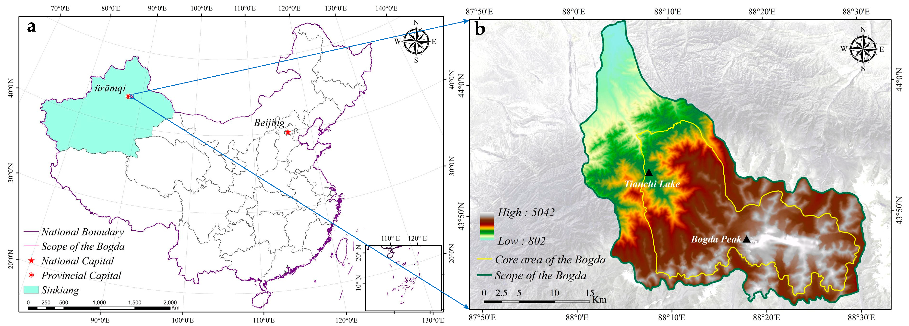
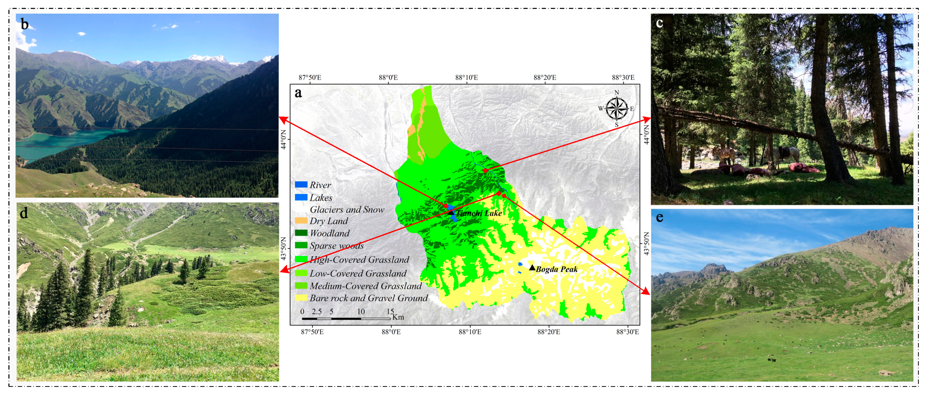
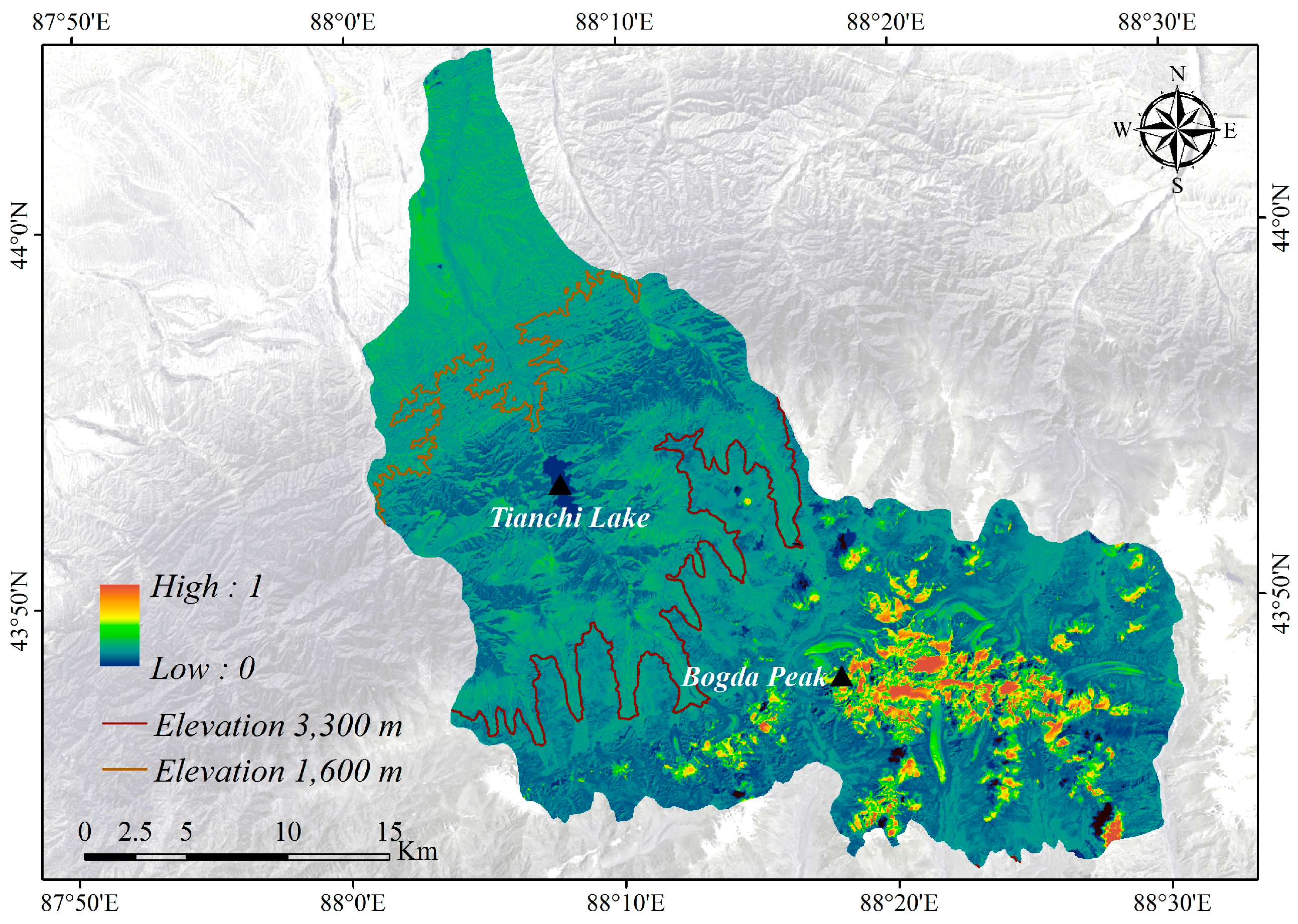
2.1. Study Area
2.2. Data
2.2.1. Landsat Data
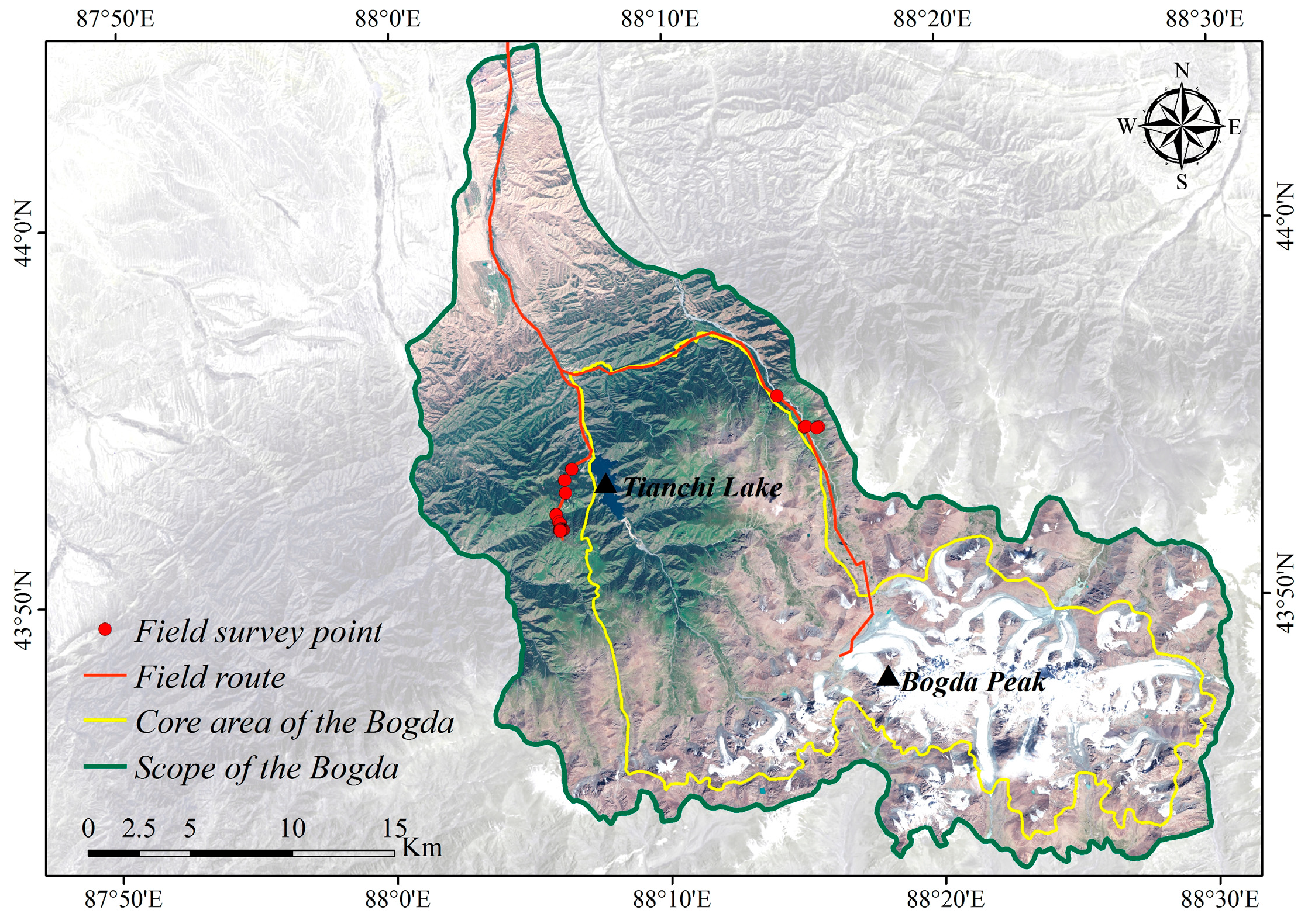
2.2.2. Field Data
2.2.3. Other Data
2.3. Methods
2.3.1. Mono-Window Algorithm
2.3.2. Total Shortwave Broadband Albedo
2.3.3. Statistical and Frequency Distribution Analysis
2.3.4. Potential Analysis
3. Results and Analysis
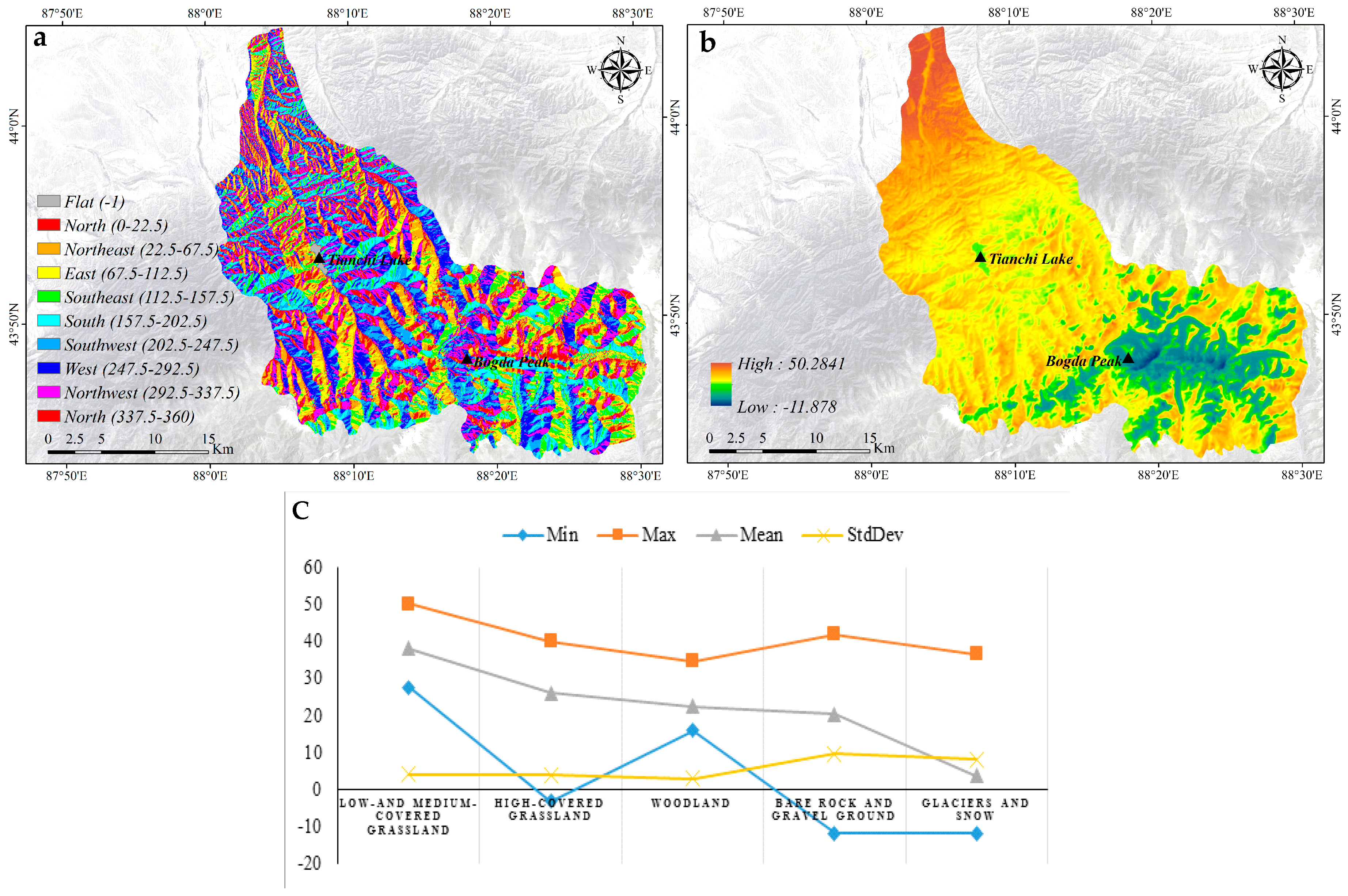
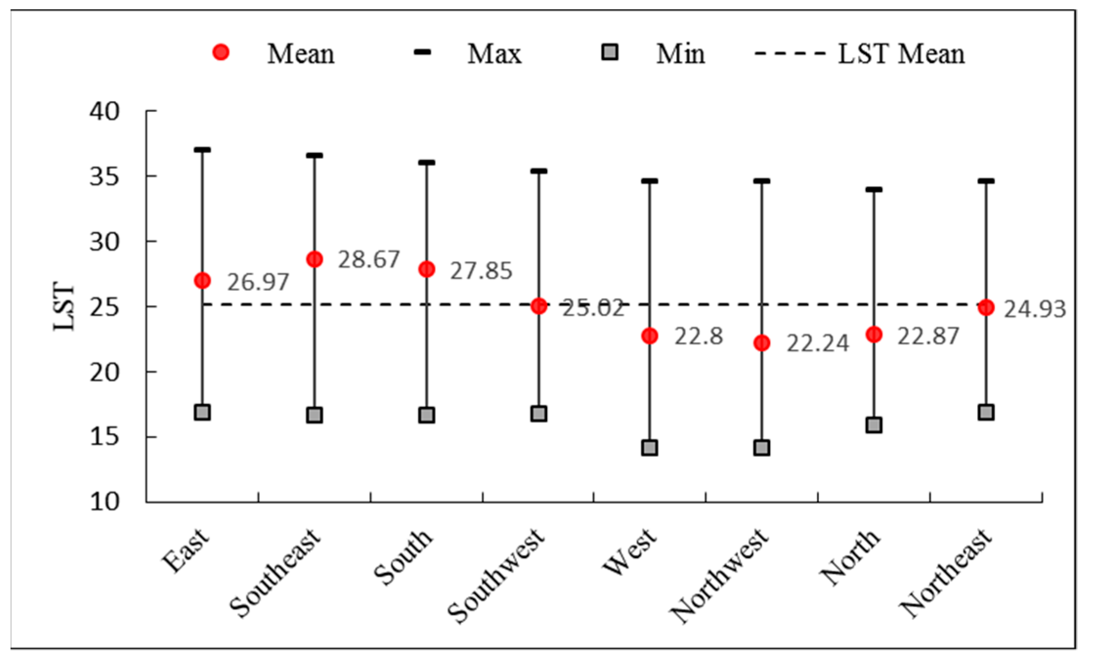
3.1. Relationship Analysis for the LST and Aspect
3.2. Critical Transitions in Altitudinal Zonality
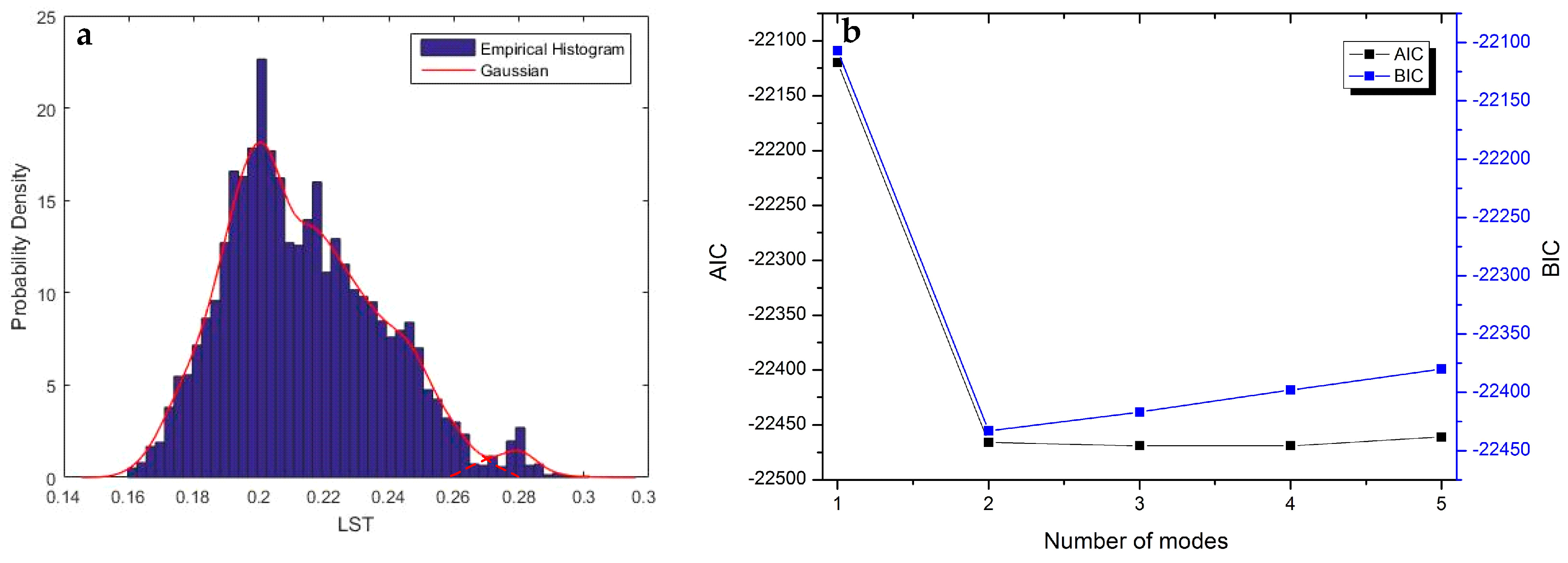
3.2.1. LST Revealed the Presence of Two States
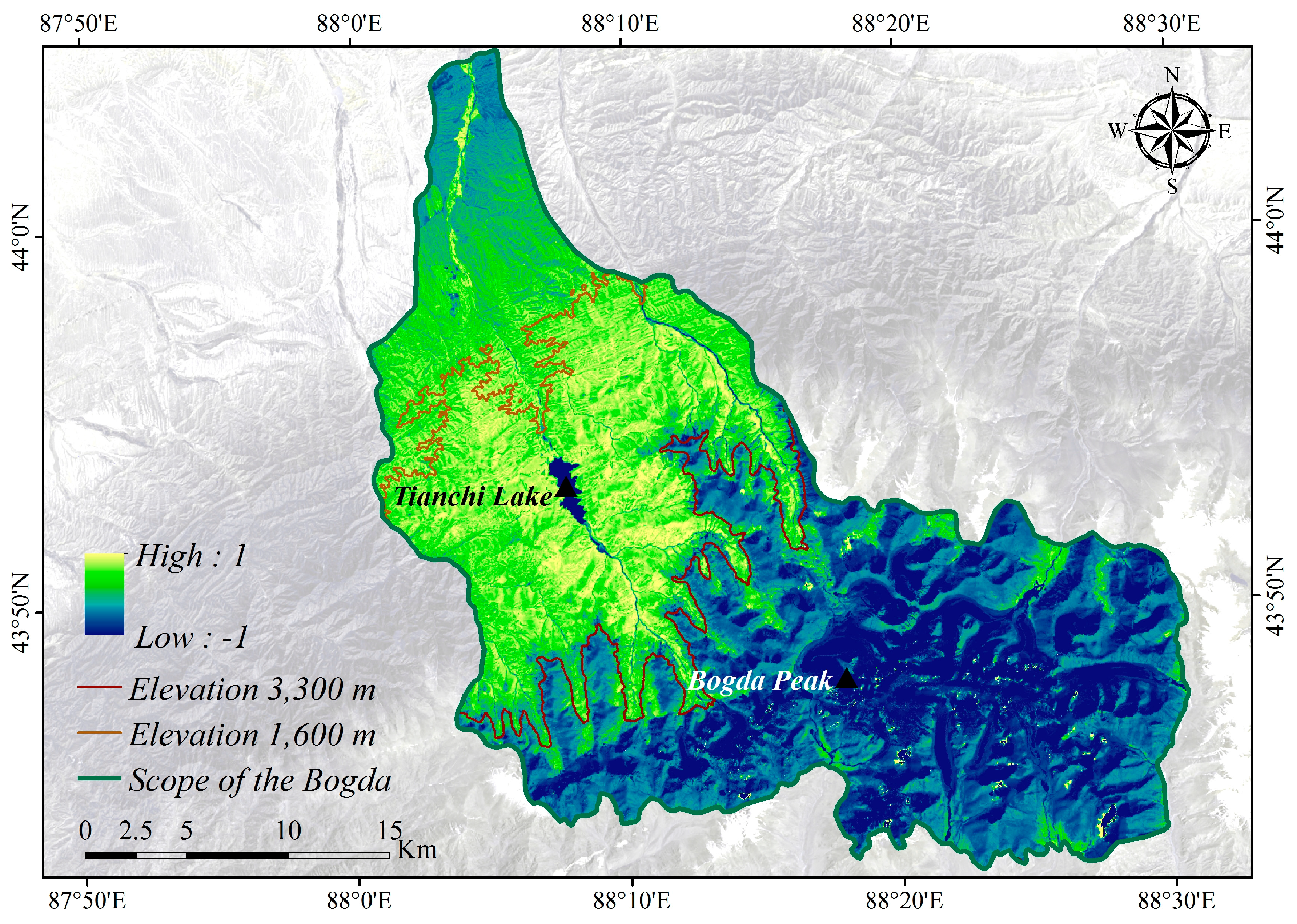
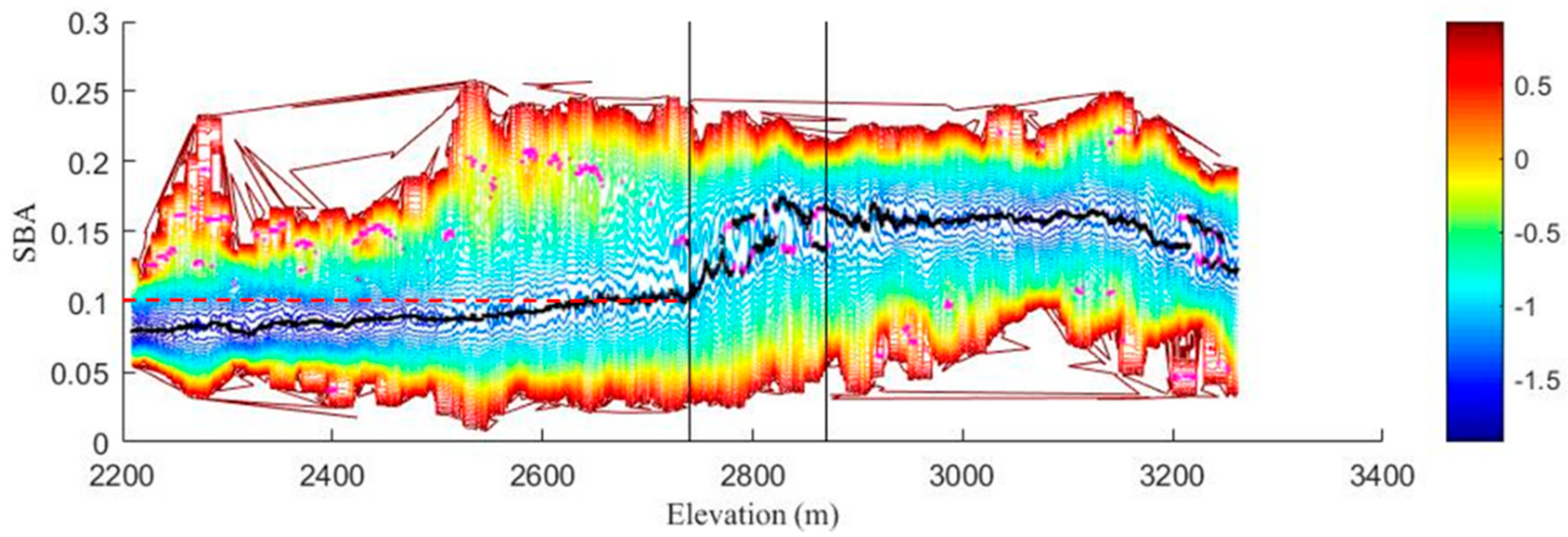
3.2.2. Detecting the Elevation Range of the Transition
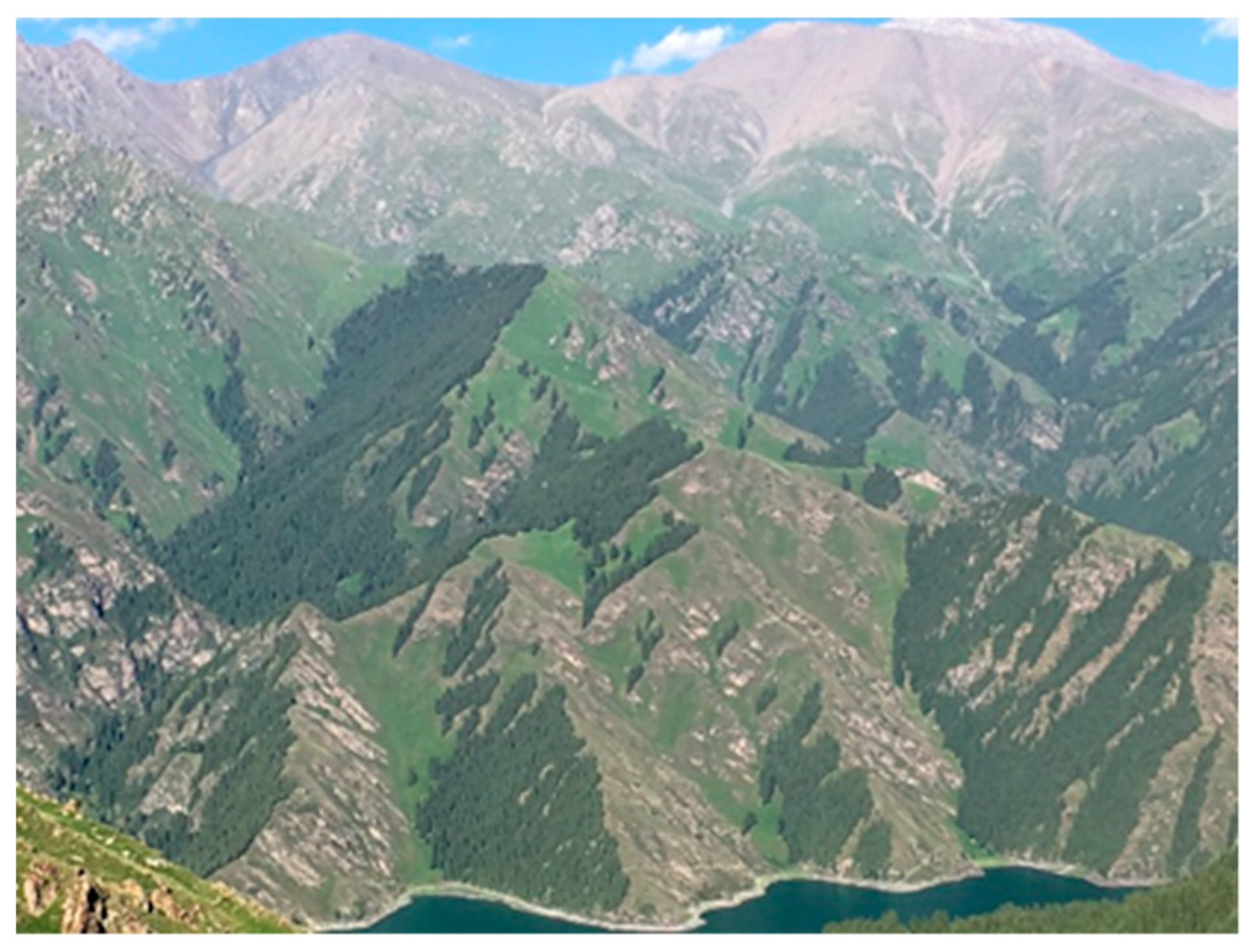
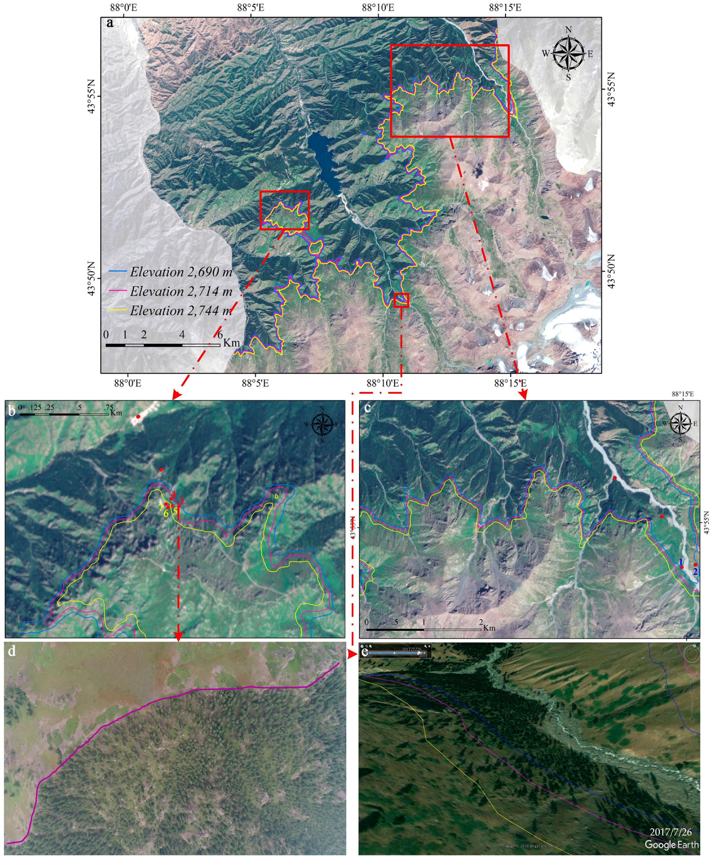
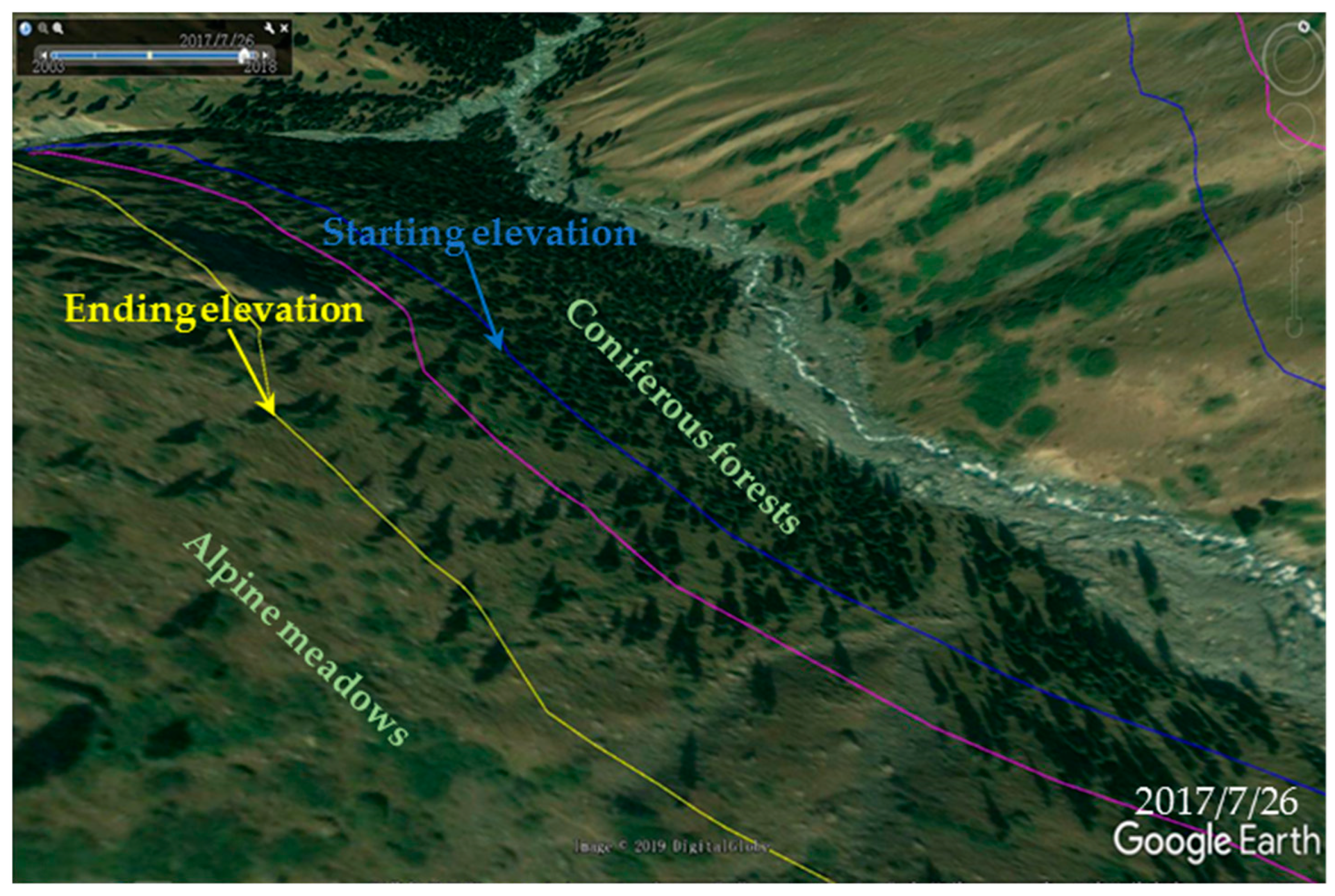
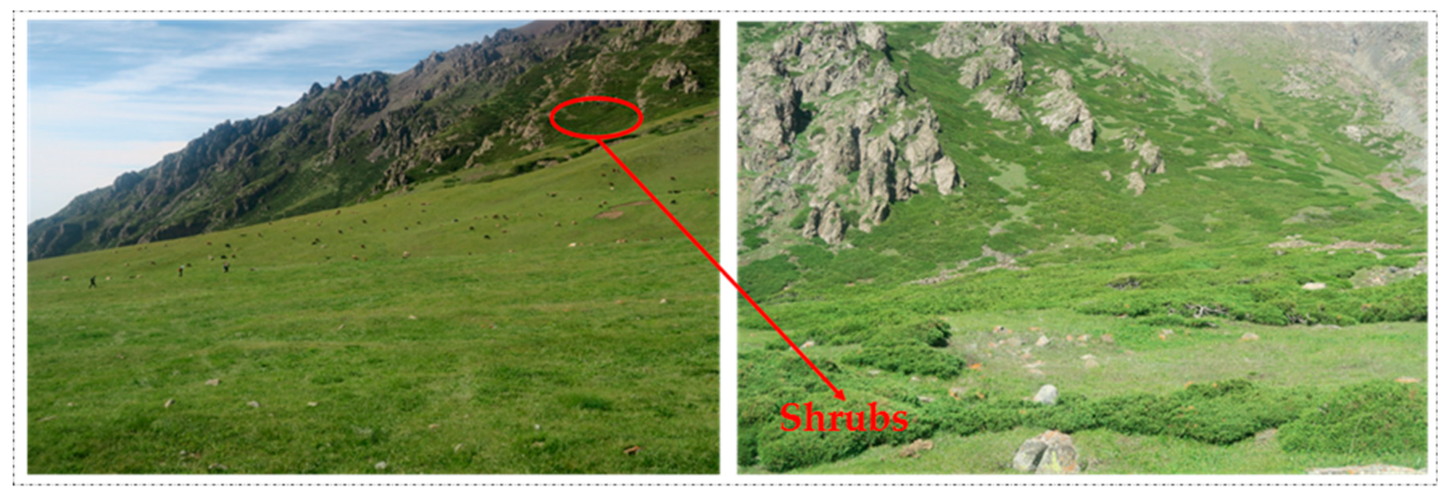
3.3. Field Validation
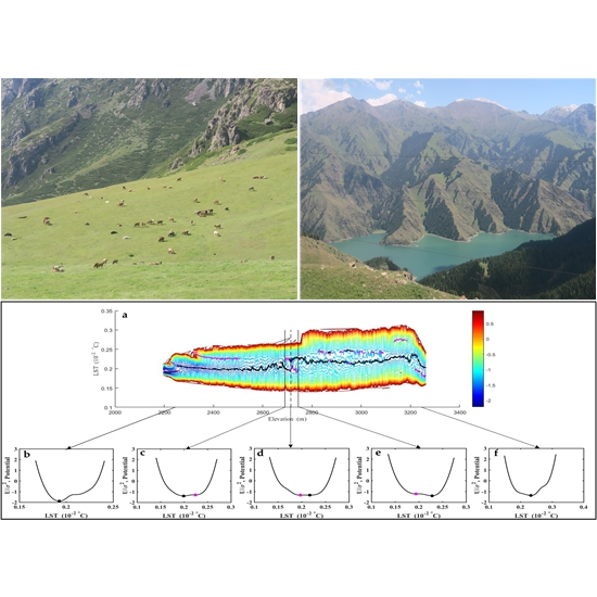
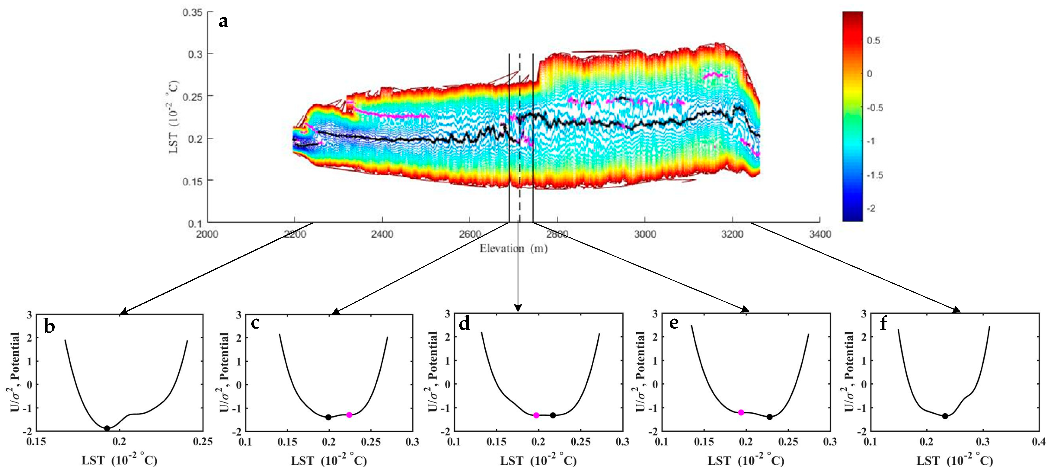
3.4. Potential Analysis of the SBA
4. Discussion
5. Conclusions
Author Contributions
Funding
Acknowledgments
Conflicts of Interest
References
- Villalba, R.; Veblen, T.T.; Ogden, J. Climatic Influences on the Growth of Subalpine Trees in the Colorado Front Range. Ecology 1994, 75, 1450–1462. [Google Scholar] [CrossRef]
- Körner, C. A re-assessment of high elevation treeline positions and their explanation. Oecologia 1998, 115, 445–459. [Google Scholar] [CrossRef] [PubMed]
- Holtmeier, F. Mountain Timberlines-Ecology, Patchiness, and Dynamics; Kluwer Academic Publishers: Dordrecht, The Netherlands, 2003. [Google Scholar]
- IPCC. Climate Change 2014: Synthesis Repot; IPCC: Geneva, Switzerland, 2014. [Google Scholar]
- Kikvidze, Z. Plant Species Associations in Alpine-Subnival Vegetation Patches in the Central Caucasus. J. Veg. Sci. 1993, 4, 297–302. [Google Scholar] [CrossRef]
- Baker, W.; Honaker, J.; Weisberg, P. Using aerial photography and GIS to map the forest-tundra ecotone in Rocky Mountain National Park, Colorado, for global change research. Photogramm. Eng. Remote Sens. 1995, 61, 313–320. [Google Scholar]
- Kupfer, J.A.; Cairns, D.M. The suitability of montane ecotones as indicators of global climatic change. Prog. Phys. Geog. 2016, 20, 253–272. [Google Scholar] [CrossRef]
- Daubenmire, R. Alpine Timberlines in the Americas and Their Interpretation. Butl. Univ. Bot. Studies 1954, 11, 119–136. [Google Scholar]
- Tranquillini, W. Physiological Ecology of the Alpine Timberline Tree, Existence at High Altitudes with Special Reference to the European Alps; Springer: Berlin/Heidelberg, Germany, 1979. [Google Scholar]
- Jobbágy, E.G.; Jackson, R.B. Global Controls of Forest Line Elevation in the Northern and Southern Hemispheres. Glob. Ecol. Biogeogr. 2000, 9, 253–268. [Google Scholar] [CrossRef]
- Körner, C.; Paulsen, J. A World-Wide Study of High Altitude Treeline Temperatures. J. Biogeogr. 2004, 31, 713–732. [Google Scholar] [CrossRef]
- Wang, X.; Zhang, L.; Fang, J. Geographical Differences in Alpine Timberline and Its Climatic Interpretation in China. China Acta Geogr. Sin. 2004, 59, 871–879. [Google Scholar]
- Lloyd, A.H.; Graumlich, L.J. Holocene Dynamics of Treeline Forests in the Sierra Nevada. Ecology 1997, 78, 1199–1210. [Google Scholar] [CrossRef]
- Perkins, T.D.; Adams, G.T. Rapid freezing induces winter injury symptomatology in red spruce foliage. Tree Physiol. 1995, 15, 259–266. [Google Scholar] [CrossRef] [PubMed]
- Wardle, P. An explanation for alpine timberline. N. Z. J. Bot. 1971, 9, 371–402. [Google Scholar] [CrossRef]
- Grace, J. Cuticular water loss unlikely to explain tree-line in Scotland. Oecologia 1990, 84, 64–68. [Google Scholar] [CrossRef] [PubMed]
- Sigdel, S.R.; Wang, Y.; Camarero, J.J.; Zhu, H.; Liang, E.; Peñuelas, J. Moisture-mediated responsiveness of treeline shifts to global warming in the Himalayas. Glob. Chang. Biol. 2018, 24, 5549–5559. [Google Scholar] [CrossRef]
- Zhang, Y.; Kun, Z.; Yan, S.; Yang, Z.; Ni, J. Late Holocene Spruce Forest Line Change and Palaeoenvironmental Characteristics on the Northern Slope of Tianshan Mountains. Chin. Sci. Bull. 2006, 51, 1450–1458. [Google Scholar]
- McLeod, T.K.; MacDonald, G.M. Postglacial Range Expansion and Population Growth of Picea mariana, Picea glauca and Pinus banksiana in the Western Interior of Canada. J. Biogeogr. 1997, 24, 865–881. [Google Scholar] [CrossRef]
- Camarero, J.J.; Gutiérrez, E.; Fortin, M. Spatial pattern of subalpine forest-alpine grassland ecotones in the Spanish Central Pyrenees. Forest. Ecol. Manag. 2000, 134, 1–16. [Google Scholar] [CrossRef]
- Panigrahy, S.; Anitha, D.; Kimothi, M.; Singh, S. Timberline change detection using topographic map and satellite imagery. Trop. Ecol. 2010, 51, 87–91. [Google Scholar]
- Yu, P.; Liu, H.; Cui, H. Vegetation and Its Relation with Climate Conditions near the Timberline of Beitai, the Xiaowutai Mts. Northern China. Chin. J. Appl. Ecol. 2002, 13, 523–528. [Google Scholar]
- Ran, F.; Liang, Y.; Yang, Y.; Yang, Y.; Wang, G. Spatial-temporal dynamics of an Abies fabri Population near the alpine treeline in the Yajiageng area of Gongga Mountain. China Acta Ecol. Sin. 2014, 34, 6872–6878. [Google Scholar]
- Han, F.; Zhang, B.; Tan, J.; Zhu, Y.; Yao, Y. The Effect of Mountain Base Elevation on the Altitude of Timberline in the Southeastern Eurasia: A Study on the Quantification of Mass Elevation Effect. China Acta Geogr. Sin. 2010, 65, 781–788. [Google Scholar]
- Král, K. Classification of Current Vegetation Cover and Alpine Treeline Ecotone in the Praděd Reserve (Czech Republic), Using Remote Sensing. Mt. Res. Dev. 2009, 29, 177–183. [Google Scholar] [CrossRef]
- Kimball, K.D.; Weihrauch, D.M. Alpine Vegetation Communities and the Alpine-Treeline Ecotone Boundary in New England as Biomonitors for Climate Change. In Wilderness as a Place for Scientific Inquiry, Proceedings of RMRS-P-15-VOL-3, Missoula, MT, USA, 23–27 May 1999; McCool, S.F., Cole, D.N., Borrie, W.T., O’Loughlin, J., Eds.; U.S. Department of Agriculture, Forest Service, Rocky Mountain Research Station: Ogden, UT, USA, 2000. [Google Scholar]
- Luo, G.; Dai, L. Detection of alpine tree line change with high spatial resolution remotely sensed data. J. Appl. Remote Sens. 2013, 7, 73520. [Google Scholar] [CrossRef]
- Singh, C.P.; Panigrahy, S.; Thapliyal, A.; Kimothi, M.M.; Soni, P.; Parihar, J.S. Monitoring the alpine treeline shift in parts of the Indian Himalayas using remote sensing. Curr. Sci. India 2012, 102, 559–562. [Google Scholar]
- Moris, J.V.; Vacchiano, G.; Ascoli, D.; Motta, R. Alternative stable states in mountain forest ecosystems: The case of European larch (Larix decidua) forests in the western Alps. J. Mt. Sci. Engl. 2017, 14, 811–822. [Google Scholar] [CrossRef]
- Woodward, F.I.; Körner, C.; Crabtree, R.C. The dynamics of leaf extension in plants with diverse altitudinal ranges: I. Field observations on temperature responses at one altitude. Oecologia 1986, 70, 222–226. [Google Scholar] [CrossRef]
- Körner, C.; Woodward, I. The dynamics of leaf extension in plants with diverse altitudinal ranges—II Field studies in Poa species between 600 and 3200 m altitude. Oecologia 1987, 72, 279–283. [Google Scholar] [CrossRef]
- Li, Y.; Luo, G.; Zhou, D.; Yin, C.; Han, Q. Eco-geographical Characteristics of Alpine Timberlines on Northern Slope of Tianshan Mountains. J. Desert Res. 2012, 32, 122–131. [Google Scholar]
- Wang, T. Ecological Study on Picea schrenkiana Forest along an altitudinal gradient in the central Tianshan Mountains. Ph.D. Thesis, Wuhan University, Wuhan, China, 2004. [Google Scholar]
- Chronopoulos, K.I.; Tsiros, I.X.; Alvertos, N.; Dimopoulos, I.F. Estimation of microclimatic data in remote mountainous areas using an artificial neural network model-based approach. Glob. NEST J. 2010, 12, 384–389. [Google Scholar]
- Lo, Y.; Blanco, J.A.; Seely, B.; Welham, C.; Hamish Kimmins, J.P. Generating reliable meteorological data in mountainous areas with scarce presence of weather records: The performance of MTCLIM in interior British Columbia, Canada. Environ. Model. Softw. 2011, 26, 644–657. [Google Scholar] [CrossRef]
- Wang, M. Methodology Development for Retrieving Land Surface Temperature and Near Surface Air Temperature Based on Thermal Infrared Remote Sensing. Ph.D. Thesis, University of Chinese Academy of Sciences (Institute of Remote Sensing and Digital Earth), Beijing, China, 2017. [Google Scholar]
- Li, Z.; Duan, S.; Tang, B.; Wu, H.; Ren, H.; Yan, G.; Tang, R.; Leng, P. Review of methods for land surface temperature derived from thermal infrared remotely sensed data. J. Remote Sens. 2016, 20, 899–920. [Google Scholar]
- Yang, Z.; Zhang, X. Tianshan World Natural Heritage Site in Xinjiang; Science Press: Beijing, China, 2017. [Google Scholar]
- Data Available from the U.S. Geological Survey. Available online: https://earthexplorer.usgs.gov/ (accessed on 6 May 2018).
- Wen, J.; Liu, Q.; Xiao, Q.; Liu, Q.; Li, X. Modeling the land surface reflectance for optical remote sensing data in rugged terrain. Sci. China Ser. D Earth Sci. 2008, 38, 1419–1427. [Google Scholar] [CrossRef]
- Mu, Y.; An, Y.; Wang, Z.; Gao, X. Comparison of Different Topographic Correction Models for Surface Reflectance Calculating in Rugged Terrain Area. China. Mt. Res. 2015, 33, 511–512. [Google Scholar]
- Anyamba, A.; Tucker, C.J. Analysis of Sahelian vegetation dynamics using NOAA-AVHRR NDVI data from 1981–2003. J. Arid Environ. 2005, 63, 596–614. [Google Scholar] [CrossRef]
- Fensholt, R.; Sandholt, I.; Rasmussen, M.S. Evaluation of MODIS LAI, fAPAR and the relation between fAPAR and NDVI in a semi-arid environment using in situ measurements. Remote Sens. Environ. 2004, 91, 490–507. [Google Scholar] [CrossRef]
- Xu, H. Retrieval of the Reflectance and Land Surface Temperature of the Newly-Launched Landsat 8 Satellite. Chin. J. Geophys. 2015, 58, 741–747. [Google Scholar]
- Xu, H.; Lin, Z.; Pan, W. Some Issues in Land Surface Temperature Retrieval of Landsat Thermal Data with the Single-channel Algorithm. Geomat. Inf. Sci. Wuhan Univ. 2015, 40, 487–492. [Google Scholar]
- Wang, F.; Qin, Z.; Song, C.; Tu, L.; Karnieli, A.; Zhao, S. An Improved Mono-Window Algorithm for Land Surface Temperature Retrieval from Landsat 8 Thermal Infrared Sensor Data. Remote Sens. 2015, 7, 4268–4289. [Google Scholar] [CrossRef]
- Yu, X.; Guo, X.; Wu, Z. Land Surface Temperature Retrieval from Landsat 8 TIRS—Comparison between Radiative Transfer Equation-Based Method, Split Window Algorithm and Single Channel Method. Remote Sens. 2014, 6, 9829–9852. [Google Scholar] [CrossRef]
- Jiménez-Muñoz, J.C.; Sobrino, J.A.; Skokovic, D.; Mattar, C.; Cristobal, J. Land Surface Temperature Retrieval Methods From Landsat-8 Thermal Infrared Sensor Data. IEEE Geosci. Remote Sens. Lett. 2014, 11, 1840–1843. [Google Scholar] [CrossRef]
- Qin, Z.; Zhang, M.; Arnon, K.; Pedro, B. Mono-window Algorithm for Retrieving Land Surface Temperature from Landsat TM6 data. China Acta Geogr. Sin. 2001, 56, 456–466. [Google Scholar]
- Jiménez-Muñoz, J.C. A generalized single-channel method for retrieving land surface temperature from remote sensing data. J. Geophys. Res. 2003, 108, 2015–2023. [Google Scholar] [CrossRef]
- Qin, Z.; Karnieli, A.; Berliner, P. A mono-window algorithm for retrieving land surface temperature from Landsat TM data and its application to the Israel-Egypt border region. Int. J. Remote Sens. 2010, 22, 3719–3746. [Google Scholar] [CrossRef]
- Hu, D.; Qiao, K.; Wang, X.; Zhao, L.; Ji, G. Comparison of Three Single-window Algorithms for Retrieving Land-Surface Temperature with Landsat 8 TIRS Data. Deomatics Inf. Sci. Wuhan Univ. 2017, 42, 869–876. [Google Scholar]
- Sobrino, J.A.; Jiménez-Muñoz, J.C.; Paolini, L. Land surface temperature retrieval from LANDSAT TM 5. Remote Sens. Environ. 2004, 90, 434–440. [Google Scholar] [CrossRef]
- Sobrino, J.A.; Jimenez-Munoz, J.C.; Soria, G.; Romaguera, M.; Guanter, L.; Moreno, J.; Plaza, A.; Martinez, P. Land Surface Emissivity Retrieval From Different VNIR and TIR Sensors. IEEE Trans. Geosci. Remote Sens. 2008, 46, 316–327. [Google Scholar] [CrossRef]
- Qin, Z.; Li, W.; Xu, B.; Chen, Z.; Liu, J. The Estimation of Land Surface Emissivity for Landsat TM 6. Remote Sens. Land Resour. 2004, 16, 28–32. [Google Scholar]
- Humes, K.S.; Kustas, W.P.; Moran, M.S.; Nichols, W.D.; Weltz, M.A. Variability of emissivity and surface temperature over a sparsely vegetated surface. Water Resour. Res. 1994, 30, 1299–1310. [Google Scholar] [CrossRef]
- He, T.; Liang, S.; Song, D. Analysis of global land surface albedo climatology and spatial-temporal variation during 1981–2010 from multiple satellite products. J. Geophys. Res. Atmos. 2014, 119, 10281–10298. [Google Scholar] [CrossRef]
- Liang, S. Narrowband to broadband conversions of land surface albedo I: Algorithms. Remote Sens. Environ. 2001, 76, 213–238. [Google Scholar] [CrossRef]
- Liang, S.; Wang, K.; Zhang, X.; Wild, M. Review on Estimation of Land Surface Radiation and Energy Budgets From Ground Measurement, Remote Sensing and Model Simulations. IEEE J.-Stars 2010, 3, 225–240. [Google Scholar] [CrossRef]
- Dickinson, R.E. Land Surface Processes and Climate-Surface Albedos and Energy Balance. Adv. Geophys. 1983, 25, 305–353. [Google Scholar]
- Lyons, E.A.; Jin, Y.; Randerson, J.T. Changes in surface albedo after fire in boreal forest ecosystems of interior Alaska assessed using MODIS satellite observations. J. Geophys. Res. 2008, 113. [Google Scholar] [CrossRef]
- Betts, R.A. Offset of the potential carbon sink from boreal forestation by decreases in surface Albedo. Nature 2000, 408, 187–190. [Google Scholar] [CrossRef] [PubMed]
- Shuai, Y.; Masek, J.G.; Gao, F.; Schaaf, C.B. An algorithm for the retrieval of 30-m snow-free albedo from Landsat surface reflectance and MODIS BRDF. Remote Sens. Environ. 2011, 115, 2204–2216. [Google Scholar] [CrossRef]
- Shuai, Y.; Masek, J.G.; Gao, F.; Schaaf, C.B.; He, T. An approach for the long-term 30-m land surface snow-free albedo retrieval from historic Landsat surface reflectance and MODIS-based a priori anisotropy knowledge. Remote Sens. Environ. 2014, 152, 467–479. [Google Scholar] [CrossRef]
- Liang, S.; Shuey, C.J.; Russ, A.L.; Fang, H.; Chen, M.; Walthall, C.L.; Daughtry, C.S.T.; Hunt, R. Narrowband to broadband conversions of land surface albedo: II. Validation. Remote Sens. Environ. 2003, 84, 25–41. [Google Scholar] [CrossRef]
- He, T.; Liang, S.; Wang, D.; Cao, Y.; Gao, F.; Yu, Y.; Feng, M. Evaluating land surface albedo estimation from Landsat MSS, TM, ETM +, and OLI data based on the unified direct estimation approach. Remote Sens. Environ. 2018, 204, 181–196. [Google Scholar] [CrossRef]
- Hais, M.; Kučera, T. The influence of topography on the forest surface temperature retrieved from Landsat TM, ETM + and ASTER thermal channels. ISPRS J. Photogramm. 2009, 64, 585–591. [Google Scholar] [CrossRef]
- Lou, A. Ecological Gradient Analysis and Environmental in Terpretation of Mountain Vegetation in the Middle Stretch of Tianshan Mountain. Acta Phytoecol. Sin. 1998, 22, 77–85. [Google Scholar]
- Scheffer, M.; Hirota, M.; Holmgren, M.; Van Nes, E.H.; Chapin, F.R. Thresholds for boreal biome transitions. Proc. Natl. Acad. Sci. USA 2012, 109, 21384–21389. [Google Scholar] [CrossRef] [PubMed]
- Scheffer, M.; Carpenter, S.R. Catastrophic regime shifts in ecosystems: Linking theory to observation. Trends. Ecol. Evol. 2003, 18, 648–656. [Google Scholar] [CrossRef]
- Akaike, H. A Bayesian analysis of the minimum AIC procedure. Ann. Inst. Stat. Math. 1978, 30, 9–14. [Google Scholar] [CrossRef]
- Akaike, H. A new look at the statistical model identification. IEEE Trans. Autom. Contr. 1974, 19, 716–723. [Google Scholar] [CrossRef]
- Burnham, K.P.; Anderson, D.R. Multimodel Inference. Sociol. Method Res. 2016, 33, 261–304. [Google Scholar] [CrossRef]
- Maestre, F.T.; Quero, J.L.; Gotelli, N.J.; Escudero, A.; Ochoa, V.; Delgado-Baquerizo, M.; Garcia-Gomez, M.; Bowker, M.A.; Soliveres, S.; Escolar, C.; et al. Plant Species Richness and Ecosystem Multifunctionality in Global Drylands. Science. 2012, 335, 214–218. [Google Scholar] [CrossRef]
- Livina, V.N.; Kwasniok, F.; Lenton, T.M. Potential analysis reveals changing number of climate states during the last 60 kyr. Clim. Past 2010, 6, 77–82. [Google Scholar] [CrossRef]
- Zhao, Y.; Wang, X.; Novillo, C.J.; Arrogante Funes, P.; Vázquez Jiménez, R.; Berdugo, M.; Maestre, F.T. Remotely sensed albedo allows the identification of two ecosystem states along aridity gradients in Africa. Land Degrad. Dev. 2019, 1–14. [Google Scholar] [CrossRef]
- Hirota, M.; Holmgren, M.; Van Nes, E.H.; Scheffer, M. Global resilience of tropical forest and savanna to critical transitions. Science 2011, 334, 232–235. [Google Scholar] [CrossRef]
- Xu, C.; Hantson, S.; Holmgren, M.; van Nes, E.H.; Staal, A.; Scheffer, M. Remotely sensed canopy height reveals three pantropical ecosystem states. Ecology 2016, 97, 2518–2521. [Google Scholar] [CrossRef]
- Berdugo, M.; Kéfi, S.; Soliveres, S.; Maestre, F.T. Plant spatial patterns identify alternative ecosystem multifunctionality states in global drylands. Nat. Ecol. Evol. 2017, 1, 3. [Google Scholar] [CrossRef] [PubMed]
- Scheffer, M.; Carpenter, S.R.; Foley, J.A.; Folke, C.; Walker, B. Catastrophic shifts in ecosystems. Nature 2001, 413, 591–596. [Google Scholar] [CrossRef] [PubMed]
- Scheffer, M.; Carpenter, S.R.; Lenton, T.M.; Bascompte, J.; Brock, W.; Dakos, V.; van de Koppel, J.; van de Leemput, I.A.; Levin, S.A.; van Nes, E.H.; et al. Anticipating critical transitions. Science 2012, 338, 344–348. [Google Scholar] [CrossRef] [PubMed]
- Liu, H. The Vertical Zonation of Mountain Vegetation in China. Acta Geogr. Sin. 1981, 36, 267–279. [Google Scholar]
- Lou, A.; Zhang, X. The Preliminary Analysis of the Distribution of Vegetation on the Middle Stretch of Tianshan Mountain of Xinjiang. J. Beijing Norm. Univ. 1994, 30, 540–545. [Google Scholar]
- Koukal, T.; Atzberger, C.; Schneider, W. Evaluation of semi-empirical BRDF models inverted against multi-angle data from a digital airborne frame camera for enhancing forest type classification. Remote Sens. Environ. 2014, 151, 27–43. [Google Scholar] [CrossRef]
- McElhinny, C.; Gibbons, P.; Brack, C.; Bauhus, J. Forest and woodland stand structural complexity: Its definition and measurement. For. Ecol. Manag. 2005, 218, 1–24. [Google Scholar] [CrossRef]
- Li, X. Spatiotemporal Changes of Global Land Surface Albedo from Remote Sensing Observations. Ph.D. Thesis, Northeast Normal University, Changchun, China, 2019. [Google Scholar]
- Ji, X.; Luo, L.; Wang, X.; Li, L.; Wan, H. Identification and change analysis of mountain altitudinal zone based on DEM- NDVI- Land cover classification in Tianshan Bogda Natural Heritage site. J. Geo. Inf. Sci. 2018, 20, 1350–1360. [Google Scholar]
- Vincze, I.; Pál, I.; Orbán, I.; Birks, H.H.; Finsinger, W.; Hubay, K.; Marinova, E.; Jakab, G.; Braun, M.; Biró, T. Holocene treeline and timberline changes in the South Carpathians (Romania): Climatic and anthropogenic drivers on the southern slopes of the Retezat Mountains. Holocene 2017, 27, 1613–1630. [Google Scholar] [CrossRef]
- Gamache, I.; Payette, S. Latitudinal Response of Subarctic Tree Lines to Recent Climate Change in Eastern Canada. J. Biogeogr. 2005, 32, 849–862. [Google Scholar] [CrossRef]
- Xu, C.; Van Nes, E.H.; Holmgren, M.; Kéfi, S.; Scheffer, M. Local Facilitation May Cause Tipping Points on a Landscape Level Preceded by Early-Warning Indicators. Am. Nat. 2015, 186, E81–E90. [Google Scholar] [CrossRef] [PubMed]
- Li, D.; You, Y.; Lan, F.; Chen, X. A research of tourism landscape resources evaluation and protection for Bogda World Natural Heritage Site. World Reg. Stud. 2015, 24, 159–167. [Google Scholar]


| Type | Resolution (m) | Sources |
|---|---|---|
| SRTM _1arc _v3 | 30 | U.S. Geological Survey (USGS) |
| Sentinel-2 L1C | 10 | ESA data distribution website |
| Land cover data | 30 | Data Center for Resources and Environmental Sciences, Chinese Academy of Sciences (RESDC) |
| Band i | 2 | 4 | 5 | 6 | 7 | |
|---|---|---|---|---|---|---|
| 0.356 | 0.130 | 0.373 | 0.085 | 0.072 | -- | |
| -- | -- | -- | -- | -- | −0.0018 |
| Transition Range (Elevation/m) | State Shifting (Elevation/m) | |||||
|---|---|---|---|---|---|---|
| PtID | Starting (m) | Ending (m) | Difference (m) | Demarcation (m) | Difference (m) | |
| Identified results | 2690 | 2744 | 2714 | |||
| Validation data | 1 | 2664 | −26 | |||
| 2 | 2662 | −28 | ||||
| 3 | 2718 | +4 | ||||
| 4 | 2705 | −9 | ||||
| 5 | 2732 | −12 | ||||
| 6 | 2745 | +1 | ||||
| 7 | 2757 | +13 | ||||
| Elevation (m) | ||||
|---|---|---|---|---|
| Demarcation | Starting | Ending | Difference (Demarcation) PtID 3–4 | |
| Ji’ results [81] | 2730 | -- | -- | −12, −25 |
| Our results | 2714 | 2690 | 2744 | +4, −9 |
© 2019 by the authors. Licensee MDPI, Basel, Switzerland. This article is an open access article distributed under the terms and conditions of the Creative Commons Attribution (CC BY) license (http://creativecommons.org/licenses/by/4.0/).
Share and Cite
Wan, H.; Wang, X.; Luo, L.; Guo, P.; Zhao, Y.; Wu, K.; Ren, H. Remotely-Sensed Identification of a Transition for the Two Ecosystem States Along the Elevation Gradient: A Case Study of Xinjiang Tianshan Bogda World Heritage Site. Remote Sens. 2019, 11, 2861. https://doi.org/10.3390/rs11232861
Wan H, Wang X, Luo L, Guo P, Zhao Y, Wu K, Ren H. Remotely-Sensed Identification of a Transition for the Two Ecosystem States Along the Elevation Gradient: A Case Study of Xinjiang Tianshan Bogda World Heritage Site. Remote Sensing. 2019; 11(23):2861. https://doi.org/10.3390/rs11232861
Chicago/Turabian StyleWan, Hong, Xinyuan Wang, Lei Luo, Peng Guo, Yanchuang Zhao, Kai Wu, and Hongge Ren. 2019. "Remotely-Sensed Identification of a Transition for the Two Ecosystem States Along the Elevation Gradient: A Case Study of Xinjiang Tianshan Bogda World Heritage Site" Remote Sensing 11, no. 23: 2861. https://doi.org/10.3390/rs11232861
APA StyleWan, H., Wang, X., Luo, L., Guo, P., Zhao, Y., Wu, K., & Ren, H. (2019). Remotely-Sensed Identification of a Transition for the Two Ecosystem States Along the Elevation Gradient: A Case Study of Xinjiang Tianshan Bogda World Heritage Site. Remote Sensing, 11(23), 2861. https://doi.org/10.3390/rs11232861