Interpretation of ASCAT Radar Scatterometer Observations Over Land: A Case Study Over Southwestern France

Abstract

This paper investigates to what extent soil moisture and vegetation density information can be extracted from the Advanced Scatterometer (ASCAT) satellite-derived radar backscatter (σ°) in a data assimilation context. The impact of independent estimates of the surface soil moisture (SSM) and leaf area index (LAI) of diverse vegetation types on ASCAT σ° observations is simulated over southwestern France using the water cloud model (WCM). The LAI and SSM variables used by the WCM are derived from satellite observations and from the Interactions between Soil, Biosphere, and Atmosphere (ISBA) land surface model, respectively. They permit the calibration of the four parameters of the WCM describing static soil and vegetation characteristics. A seasonal analysis of the model scores shows that the WCM has shortcomings over karstic areas and wheat croplands. In the studied area, the Klaus windstorm in January 2009 damaged a large fraction of the Landes forest. The ability of the WCM to represent the impact of Klaus and to simulate ASCAT σ° observations in contrasting land-cover conditions is explored. The difference in σ° observations between the forest zone affected by the storm and the bordering agricultural areas presents a marked seasonality before the storm. The difference is small in the springtime (from March to May) and large in the autumn (September to November) and wintertime (December to February). After the storm, hardly any seasonality was observed over four years. This study shows that the WCM is able to simulate this extreme event. It is concluded that the WCM could be used as an observation operator for the assimilation of ASCAT σ° observations into the ISBA land surface model.

1. Introduction

The main mission of space-borne radar scatterometers is to monitor wind speed over the oceans [1]. It was shown that wind scatterometers operating at the C-band frequency (~5 GHz) such as the Advanced Scatterometer (ASCAT) can be used over land to monitor variables such as surface soil moisture (SSM) [2] and vegetation optical depth (VOD) [3]. The ASCAT C-band radar VOD can be related to vegetation water content (VWC) as well as to the leaf area index (LAI) [3]. Both SSM and LAI can be integrated into land surface models (LSMs) in order to analyze key variables such as the root-zone soil moisture and the vegetation above-ground biomass. Barbu et al. [4] showed the feasibility of implementing the joint sequential assimilation of SSM and LAI into the Interactions between Soil, Biosphere, and Atmosphere (ISBA) LSM within the Surface Externalisée (SURFEX) modeling platform [5]. Their work permitted the development of a Land Data Assimilation System (LDAS). Albergel et al. [6] further extended the LDAS at a global scale (LDAS-Monde) and showed that the assimilation of LAI observations can be used to analyze the root-zone soil moisture in addition to the vegetation above-ground biomass. This also means that LDAS-Monde could potentially use the information content of C-band backscatter observations (σ°) to analyze vegetation variables together with the root-zone soil moisture [6]. To achieve this goal, an observation operator such as the water cloud model (WCM) [7] is needed for predicting σ° from LSMs. SSM and LAI observations can be assimilated into the ISBA LSM because these two variables can be predicted by ISBA. It must be noted that the current version of ISBA is not able to simulate the VWC.

The simulation of the radar backscatter signal requires a radiative transfer model that calculates the propagation of radiation (in this case, microwave radiation) through a plant canopy. In this study, the semi-empirical WCM proposed by Attema and Ulaby [7] is used to simulate the impact of SSM and LAI on the total radar backscatter signal σ°. Lievens et al. [8] used a version of the WCM to simulate ASCAT σ° from simulated SSM values and VOD observations from passive microwave instruments. Vreugdenhil et al. [3] showed that C-band VOD values derived from ASCAT σ° using the WCM are correlated with satellite-derived LAI observations from the Copernicus Global Land service [9] over Australia. The VOD versus LAI correlation was particularly good for grasslands, but a time lag was observed for crops and forests. A possible explanation for the mismatch between VOD and LAI time series was that VOD at C-band may be sensitive to non-photosynthetic vegetation parts (e.g., branches in the case of forests) in addition to leaves. Finally, the WCM may not be able to represent all components of scattering within vegetation canopies [10].

The objectives of this study are to investigate

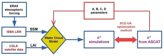
• The ability of the WCM to simulate ASCAT σ° observations using SSM values simulated by the ISBA LSM and satellite-derived LAI, in contrasting land-cover conditions over southwestern France,
• The statistical distribution of the parameters of the WCM,
• The response of observed and simulated σ° to LAI and SSM across seasons,
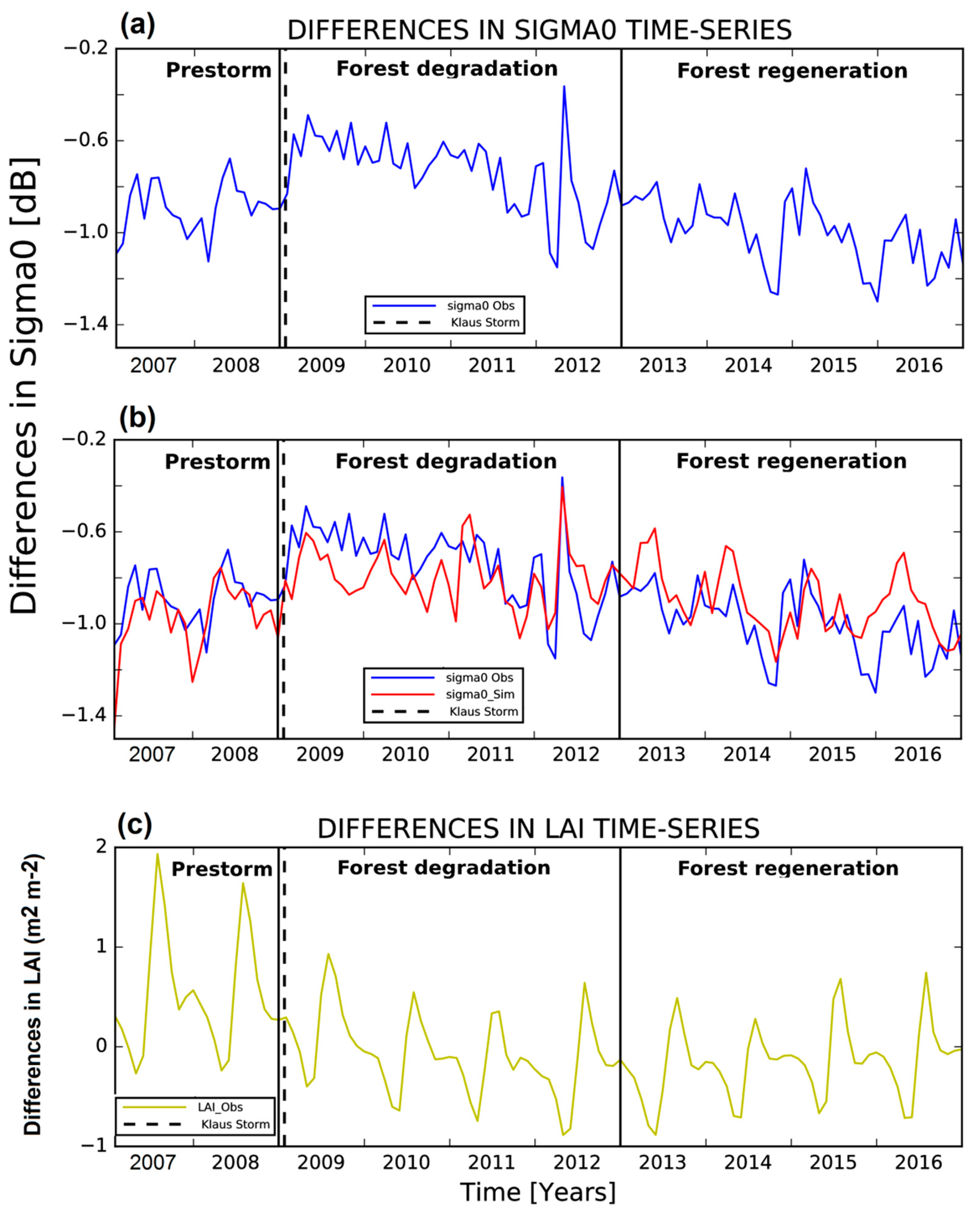
• The response of observed and simulated σ° to a rapid change in vegetation cover, and
• The feasibility of building an observation operator for the assimilation of ASCAT σ° observations into the ISBA LSM.

In a first stage, a standard calibration method is used in order to fit the parameters of the WCM. The calibrated WCM is evaluated using σ° observations not used during the calibration process. In a second stage, the capacity of σ° observations to detect vegetation changes and the capacity of the WCM to simulate such impacts on σ° are evaluated over an area of the Landes forest affected by the Klaus windstorm event of 24 January 2009.

The data and methods are presented in Section 2. The results are presented in Section 3 and discussed in Section 4. Finally, the main conclusions are summarized in Section 5.

2. Material and Methods

2.1. Study Area

The study area is located in southwestern France, 42.00° N to 46.00° N and 2.00° W to 4.00° E (Figure 1). The main vegetation types consist of crops such as maize and wheat, grasslands, coniferous trees, and broadleaf trees [11]. The large Landes coniferous forest covers the western part of the domain. The Landes forest mainly consists of maritime-pine (Pinus pinaster) trees in sandy soils [12]. This forest was damaged by the Klaus windstorm event of 24 January 2009. The “Storm” zone (43.80° N−44.25° N, 1.00° W−0.40° W) indicated in Figure 1 corresponds to the forest area that was most affected by Klaus [13]. Two zones, “North” (44.55° N−45.00° N, 0.75° W−0.15° W) and “South” (43.40° N−43.85° N, 0.30° W−0.30° E), are also selected for further analysis of the impact of Klaus, following Teuling et al. [13]. These two zones are mainly composed of crop and grassland land-cover types, with the North zone also including urban and forested areas. The South zone corresponds to the Bas-Armagnac agricultural area. Agricultural areas present contrasting crop rotation systems. For example, the south of the Landes forest (including Bas-Armagnac) is mainly covered by maize monoculture, with some areas covered by vineyards. Grassland and forest patches are found over the steepest slopes. Further east, C3 crops such as wheat are dominant. This is the case of the Lomagne agricultural area. Crop rotation in Lomagne is characterized by winter crops such as wheat, barley, and rapeseed and summer crops such as maize, sorghum, and sunflower. Areas presenting a mean elevation greater than 1200 m above sea level (a.s.l.) are excluded from the analysis. They are found in the Pyrenees Mountains.

2.2. SSM Simulations

The ISBA LSM was developed at the National Center for Meteorological Research (CNRM) and is a part of the SURFace Externalisée (SURFEX) modeling platform of Meteo-France [5]. In this study, a carbon dioxide responsive version of the ISBA LSM [14,15] in SURFEX version 8.1 is used to simulate SSM together with the surface soil ice content and LAI. Only SSM is used in this work, from the model topsoil layer comprised between 1 and 4 cm depth. The simulated topsoil temperature and ice content in the shallow (1 cm thick) surface soil layer are used to exclude soil-freezing conditions from the analysis. The ISBA model runs are driven by ERA-5 [16], which is the latest atmospheric reanalysis from the European Center For Medium-Range Weather Forecast (ECMWF). The ISBA simulations cover southwestern France from 2007 to 2016 at a spatial resolution of 0.25° × 0.25°.

2.3. ASCAT σ° Observations

ASCAT is a real aperture radar on board the Meteorological Operational Satellite Program of Europe (Metop) series of satellites. It operates at a frequency of 5.255 GHz in C-band and uses vertically polarized antennas for transmission and reception, producing like-polarized VV radar backscatter (σ°) observations. The first Metop satellite, called Metop-A, has been operational since 2006. Metop-B and Metop-C were launched in 2012 and 2018, respectively. The ASCAT sensors have two sets of three antennae, measuring σ° at three azimuth angles of 45°, 90°, and 135° over two 550 km wide swaths separated by a gap of about 360 km from the satellite ground track for a minimum orbit height. Measurements of σ° are done over a wide range of incidence angles varying from 25° to 65°. The ASCAT backscatter observations are available at full resolution, together with spatially weighted measurements at 25 km × 25 km or 50 km × 50 km resolution [2,17]. In this study, we used an ASCAT σ° dataset normalized to an incidence angle of 40°, which was provided by the Vienna University of Technology. The dataset is sampled on a discrete global grid (12.5 km × 12.5 km) at a spatial resolution of 25 km × 25 km. The incidence angle normalization is done by using a second-order polynomial describing the relationship between incidence angle and backscatter [18]. The σ° dataset consists of mean daily values incorporating data from ascending and descending orbits. In order to adapt the normalized ASCAT σ° data to the 0.25° × 0.25° grid used by the ISBA model, the data were interpolated by an arithmetic average to the model grid points. Further processing was made to mask the ASCAT σ° data for areas with frozen soils and very complex topography so as to avoid these perturbing factors influencing the results.

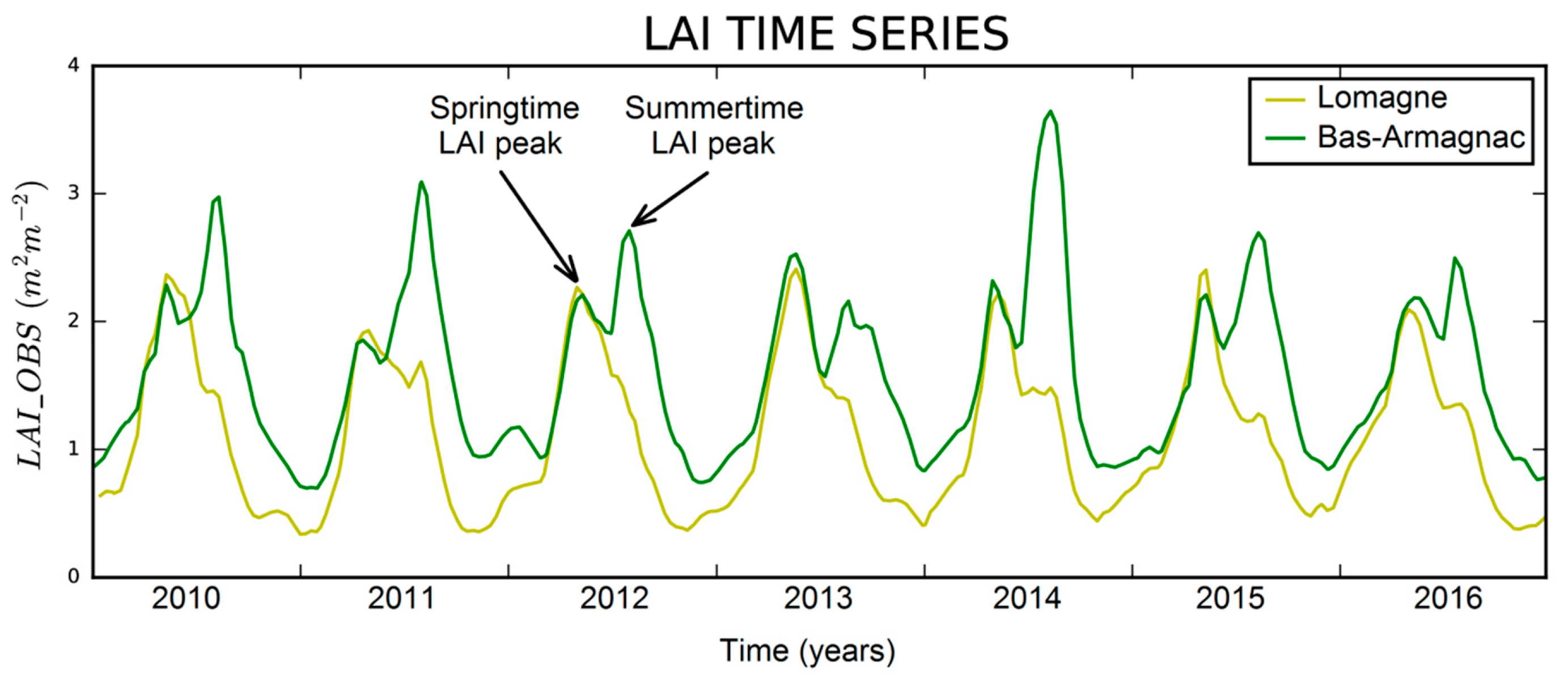
2.4. LAI Observations

The satellite-derived LAI product referred to as GEOV2 is produced by the Copernicus Global Land Service (CGLS) (http://land.copernicus.eu/global/). The GEOV2 LAI is available every 10 days at a spatial resolution of 1 km × 1 km. A neural network retrieval technique [9] is used to derive the GEOV2 LAI product from SPOT-VGT sensors (from 1999 to 2014) and PROBA-V sensors (from 2014 to present). Validation studies made by Camacho et al. [19] demonstrated that this LAI product tends to perform better than other products, with a root mean square deviation (RMSD) with respect to in situ observations across contrasting biomes of about 0.7 m²m⁻². This LAI product was integrated into the ISBA LSM in a number of studies [6,20,21] using a sequential data assimilation technique. In this study, the LAI product was interpolated by an arithmetic average to the 0.25° × 0.25° model grid points. A discussion on the added value of this product can be found in Section 4.4.

2.5. The Water Cloud Model (WCM)

Several models can be used to model radar backscatter signals over land [22,23,24]. The WCM stands out as a robust approach because of its simplicity: it needs few parameters to be fitted and uses few biophysical variables. It can be used as an inversion model to retrieve vegetation and soil moisture variables at various wavelengths [25,26,27,28,29,30,31]. The WCM assumes that the vegetation canopy can be modeled as a collection of water droplets that are uniformly distributed within the canopy. Generally, the radar backscattering from a vegetated soil surface comprises (1) the direct backscatter of the vegetation $({\sigma }_{veg}^0)$, (2) the backscatter of the soil $({\sigma }_{soil}^0)$, which is attenuated twice by the vegetation layer, in relation to the vegetation transmissivity (t) depending on the incidence angle (θ) and on the vegetation optical depth (VOD), and (3) multiple scattering from vegetation–ground interactions $({\sigma }_{veg+soil}^0)$:

$${\sigma }_{}^0={\sigma }_{veg}^0+t^2{\sigma }_{soil}^0+{\sigma }_{soil+veg}^0$$

(1)

with

$${\sigma }_{soil (dB)}^0=10lo{g}_{10}{\sigma }_{soil}^0=C+D\times SSM$$

(2)

$$t=e^{- \frac{VOD}{\cos \theta }}$$

(3)

$${\sigma }_{veg}^0=A V_1\cos \theta (1-t^2)$$

(4)

and

$$VOD=B V_2.$$

(5)

It must be noted that in Equations (1) and (2), ${\sigma }_{soil}^0$ is expressed in linear units, while in Equation (2), ${\sigma }_{soil(dB)}^0$ is expressed in dB units. SSM is the volumetric soil moisture, which in this study is representative of the top 1–4 cm layer of the soil in the ISBA LSM.

It is assumed that the double-bounce term can be neglected:

$${\sigma }_{veg+soil}^0\ll {\sigma }^0.$$

(6)

Since the WCM is a semi-empirical model, the vegetation structure is not represented in detail. Instead, the $V_1$ and $V_2$ variables represent the impact of vegetation on σ°. They can be related to the VWC or to proxies of the VWC such as LAI or vegetation indices (e.g., the normalized difference vegetation index, NDVI). In the original WCM [7] $V_1$ is set as $V_1$ = 1. In other studies, the same vegetation variable such as LAI or VWC is used for both $V_1$ and $V_2$ (for example [8,24,30,32]). Other authors proposed to use different variables to act as $V_1$ and $V_2$ [25,33,34].

In this study, $V_1$ was set as $V_1$ = 1 and LAI was used as a proxy for VWC [30]:

$$\{\begin{array}{c}{V}_1=1\\ V_2=LAI\end{array} .$$

(7)

Preliminary tests have shown that Equation (7), corresponding to the original WCM [7], gives better results than other options over southwestern France.

The WCM (Equations (1)–(7)) contains four static parameters whose values may change from one area to another. The A and B parameters in Equations (4)–(5), which are dimensionless, are related to vegetation properties. There is no universal theoretical method to characterize the best group of vegetation descriptors, and thus to retrieve the values of the A and B parameters [25]. These parameters depend on the canopy type and on radar configuration. The C and D parameters in Equation (2), in dB units, are related to soil properties. Parameter C is the value of the backscatter coefficient for a perfectly dry soil and is essentially controlled by the surface roughness and incidence angle. Parameter D refers to the radar sensitivity to variations in soil moisture, which depends on the radar configuration and soil characteristics.

It is interesting to note that in this configuration of the WCM (Equation (7)), there is a critical value of SSM for which only one σ° value equal to A cosθ can be simulated by the WCM, whatever the LAI value:

$$SS{M}_C=(10lo{g}_{10}(A\cos \theta )-C)/D.$$

(8)

2.6. Model Calibration

The WCM model is a semi-empirical model and its parameter values A, B, C, and D at a given grid cell must be estimated by calibrating the model against observations. In order to avoid the impact of changes in the vegetation coverage caused by the Klaus storm in early 2009, the time period before the storm and during 2009 is not accounted for in the WCM calibration over southwestern France. Instead of the whole 2007–2016 time period, only the 2010–2016 subset is considered for calibration and validation. To assess the robustness of the calibrated WCM parameters, the σ° simulations of the calibrated WCM are compared with the σ° observations that are not used in the calibration. The calibration and the validation are performed during the 2010–2013 and 2014–2016 time periods, respectively. In order to check the stability of the retrieved parameter values, an additional calibration is performed over a longer period of time (2010–2016) encompassing the initial calibration period and the validation period.

Al-Yaari et al. [35] derived L-band VOD estimates from SMOS (Soil Moisture and Ocean Salinity) observations. Assuming that the L-band VOD is a proxy for standing biomass, they showed that the impact of Klaus on the Landes forest biomass, including the impact of forestry work following the storm, was pronounced until the end of 2012. In this study, we investigate to what extent the Klaus event can be observed by ASCAT. In addition to the whole WCM calibration over southwestern France, a specific calibration for the storm area of the Landes forest (Figure 1) is performed for three time periods: pre-storm (January 2007 to 24 January 2009), forest degradation (25 January 2009 to December 2012), and forest regeneration (2013–2016).

For retrieving the values of the WCM parameters, the calibration process is done by comparing simulated and observed σ° values expressed in linear units. In field experiments where homogeneous land-cover conditions can be ensured, the two soil parameters (C and D) can be obtained over bare soil by a linear model fitting as expressed in Equation (2) [7]. This method cannot be used for the low-resolution ASCAT σ° observations from space, because the large ASCAT pixels may include various land-cover types, bare soil, and vegetated surfaces.

In this study, an approach consisting of simultaneously retrieving A, B, C, and D is used. A cost function K as expressed in Equation (9) is minimized.

$$K=\sqrt{\frac{1}{N}{\displaystyle \sum }_i^N{({\sigma }_{mod}^0-{\sigma }_{obs}^0)}^2}+W_{\alpha }\frac{1}{N_{\alpha }}{\displaystyle \sum }_i^{N_{\alpha }}\frac{{({\alpha }_{0,i}-{\alpha }_i)}^2}{{\sigma }_{{\alpha }_{(0,i)}}^2}$$

(9)

In Equation (9), the cost function incorporates the backscatter coefficients predicted by the water cloud model $({\sigma }_{mod}^0)$ and those observed by ASCAT $({\sigma }_{obs}^0)$, which are all in linear units, along with a parameter penalty. The N symbol represents the number of σ° simulations and observations, $N_{\alpha }$ represents the number of fitted WCM parameters, $W_{\alpha }$ represents the weight factor given to the parameter penalty term, ${\alpha }_i$ represents the i^th parameter value, and ${\alpha }_{i,0}$ represents the prior value of the i^th parameter. The minimization is performed using the Shuffled Complex Evolution Algorithm (SCE-UA) method [36]. The SCE-UA method is widely used and has proven as being robust and effective for fitting model parameters [37]. Lievens et al. [8] successfully used this technique to calibrate WCM parameters at a global scale. We use the same weight-factor value set to 0.01 as in [8]. The variance of each parameter ${\sigma }_{{\alpha }_{(0,i)}}^2$ is assumed to be equal to the variance of a uniform distribution as expressed in Equation (10) with boundaries $\left[{\alpha }_{max,i},{\alpha }_{min,i}\right]$ set as in [38].

$${\sigma }_{{\alpha }_{(0,i)}}^2=\frac{{({\alpha }_{max,i}-{\alpha }_{min,i})}^2}{12}$$

(10)

The prior and boundaries values of the dimensionless WCM parameters are fixed as those given in Table 2 of [8].

The implementation of the model calibration is illustrated in Figure 2.

2.7. Implementation of σ° Simulations

The calibrated WCM is used to produce σ° simulations over southwestern France from 2010 to 2016, using the SSM simulations and LAI observations described in Section 2.2 and Section 2.4, respectively. In order to remove the impact of soil-freezing conditions on the comparison with the observed ASCAT σ°, regions presenting simulated topsoil surface temperature below 2 °C and ice are masked out. Specific simulations are used to investigate the impact of the Klaus storm on the Landes forest by using a time series of the mean simulated σ° values over the North, Storm, and South zones (Figure 1) from 2007 to 2016.

2.8. Statistical Analysis

The WCM model results for σ° are compared to satellite observations measurements using the Pearson correlation coefficient (R) and the RMSD. While the observed and simulated σ° from the WCM is expressed in linear units during the calibration process, values expressed in dB units are used for calculating the R and RMSD scores.

The analysis of the impact of the Klaus storm is based on the North, Storm, and South zones in Figure 1 (Section 2.1), as defined by [13]. Following the method used by [13] to assess differences in cloud coverage between forest and non-forest areas, the difference in σ° between the Storm zone and the average of the North and South zones is investigated. The difference is calculated for the ASCAT observations, and for the WCM simulations.

$$Dif{f}_{{\sigma }^0}={\sigma }_{stormzone}^0-\frac{({\sigma }_{northzone}^0+{\sigma }_{southzone}^0)}{2}$$

(11)

We used the forest σ° difference with neighboring areas in order to eliminate the weather factor. Preliminary tests based on a simple time series of σ° over the Landes forest showed that the impact of the storm was not clearly visible. The σ° values are sensitive to rainfall events, and the storm impact on the signal is masked by the weather factor. Using the difference with neighboring areas as in [13] tends to eliminate this factor. We do not focus on the same subject as addressed by [13], but we follow the same protocol to highlight differences in the geophysical variables.

3. Results

3.1. Parameter Values

Retrieved A and B vegetation parameter values range from 0.07 to 0.20 and from 0.2 to 1.7, respectively (

Table 1. Water cloud model (WCM) parameters (A, B, C, and D) over southwestern France: minimum, median, and maximum values, together with standard deviation and skewness scores.

Time period	Parameter	Median [Minimum, Maximum]	Standard deviation	Skewness
2010–2013 (calibration period)	A	0.14 [0.07, 0.20]	0.02	–0.51
	B	0.36 [0.20, 1.71]	0.21	2.30
	C (dB)	−17.9 [−20.0, −15.1]	0.8	0.10
	D (dB)	27.9 [24.9, 29.7]	0.7	–0.66
2010–2016	A	0.14 [0.07, 0.20]	0.02	–0.49
	B	0.41 [0.22, 1.50]	0.19	1.93
	C (dB)	−17.6 [−20.0, −14.9]	0.8	–0.04
	D (dB)	28.0 [24.9, 29.7]	0.6	–0.62

). Figure 3 shows the probability distribution of parameter values. The large skewness score for B (Table 1) indicates that the probability distribution of this parameter is not Gaussian. It presents a long tail toward large values. The most frequent B values range from 0.3 to 0.5. The largest B values are observed close to the Mediterranean coast and over C3 crops such as wheat. The latter tend to display intermediate values of A and relatively large values of B ranging mainly from 0.5 to 0.8. The statistical distribution of A corresponds to rather evenly distributed values and can be related to well-known geographic patterns. Figure 4 shows that very large values of A (close to 0.20) correspond to the wide urban areas of Toulouse and Bordeaux. Values of A around 0.17 tend to match with the large fractions of broadleaf trees in Figure 1. Small values of A (around 0.10) tend to match with the large fractions of grass and coniferous trees in Figure 1.

Regarding soil parameters C and D, Figure 4 shows that urban areas present large values for both (C > −16 dB and D > 29 dB). Meanwhile, the Landes forest presents large values of C and D (around –16 dB and 29 dB, respectively), the volcanoes of Cantal (landmark “3” in Figure 4) present very low values (around –19.5 dB and 25 dB, respectively). It must be noted that the soil types of these areas are quite different. While the Landes forest is characterized by sandy soils [12], the soils of Cantal are loamy (they are classified as Andosols in the French soil classification system [39]). Another difference between Landes and Cantal is altitude (below 150 m a.s.l. and above 900 m a.s.l., respectively) and topography (flat and complex terrain, respectively). Interestingly, low values of C are also found for mountainous karstic areas: Quercy, Corbières, Cévennes (landmarks “4”, “5”, and “6” in Figure 4, respectively).

Figure 3 and Table 1 also show that the A parameter values resulting from the calibration over a longer period of time (2010−2016) present a statistical distribution similar to the initial parameter values calibrated over 2010−2013. The histograms of the other parameters are slightly shifted toward larger values.

3.2. Performance of the WCM

The performance of the calibration of the WCM using the SCE-UA algorithm is assessed in

Table 2. WCM performance: statistical scores of simulated σ° values over southwestern France. The calibration period of the parameters is from 2010 to 2013, and the validation period is from 2014 to 2016. For both calibration and validation periods, scores are given for the pooled dataset (All) and for the March, April, and May (MAM) spring period and the June, July, and August (JJA) summer period. The number of observations is indicated (n).

Scores	R Median [Minimum, Maximum] (n)			RMSD in dB Median [Minimum, Maximum]
Seasons	All	MAM	JJA	All	MAM	JJA
Calibration (2010–2013)	0.67 [0.16,0.80] (209327)	0.60 [0.02,0.77] (45348)	0.44 [–0.18,0.71] (90082)	0.35 [0.22,0.68]	0.39 [0.23,0.86]	0.32 [0.17,0.54]
Validation (2014–2016)	0.69 [0.17,0.82] (204520)	0.60 [–0.04,0.80] (45805)	0.47 [–0.38,0.68] (83139)	0.36 [0.20,0.68]	0.36 [0.19,0.66]	0.32 [0.18,0.75]

. Simulated and observed σ° values are compared using a large number of observations (n) for the calibration and for the validation period, using the R and RMSD scores. For these two periods of time, n = 209,327 and n = 204,520 observations are available, respectively, after sorting out the soil freezing events. For each time period, two data subsets are considered in addition to the pooled dataset: springtime (i.e., in March, April, and May (MAM)) and summertime (i.e., in June, July and August (JJA)). Table 2 shows that the scores for the validation period are very close to those for the calibration period. The WCM performs better in the springtime in terms of correlation than in the summertime. While the median R value is 0.60 for the calibration period in the springtime, a value of 0.44 is obtained in the summertime. Negative values are even observed in the summertime. On the other hand, the RMSD score presents better values in the summertime. The mean model bias (not shown) is +0.11 dB in the springtime and −0.14 dB in the summertime. The WCM bias is further examined in Figure 5.

In Figure 5, maps of simulated σ° values are compared with ASCAT σ° observations for spring and for summer. The large urban areas of Toulouse and Bordeaux are clearly visible in Figure 5 because they present the largest observed σ° values. The latter correspond to the high A and C values observed in Figure 4. The temporal correlation between the WCM simulations and the observations is also shown. Again, this score tends to present better values in the springtime than in the summertime. Small or negative correlations are found in locations corresponding to the three karstic areas presented in Figure 4. The mean simulated σ° maps are quite similar to the observations (not shown), and the mean seasonal bias is generally very small. However, a seasonal bias can be observed over agricultural areas mainly covered by C3 crops (see Figure 1). An example of such an agricultural area is Lomagne (“7” in Figure 5). Over these areas, the calibrated WCM tends to overestimate σ° in the springtime and to underestimate σ° in the summertime.

Figure 6 presents the daily and monthly time series of spatially averaged simulated and observed σ° over southwestern France. It appears that the simulated ASCAT σ° values in the springtime are systematically higher than the observed ones. The σ° observations are often lower in the springtime than in the summertime. This seasonal bias is consistent with the biases observed in Figure 5 over the C3 crop areas. In spite of the seasonal mismatch between observed and simulated values, the monthly time series of scaled anomaly in Figure 6 show that the simulated month-to-month variability of σ° is consistent with the observations.

3.3. Landes Forest: Impact of the Klaus Storm

The result of the analysis method consisting of comparing the Storm area (Figure 1) with the bordering North and South agricultural areas (see Section 2.8) is presented in Figure 7. It is observed that the seasonal cycle of the monthly difference in σ° observations changes after the storm event of 24 January 2019. Before this date, the difference is small in the springtime (> −0.8 dB) and large in the autumn and wintertime (< −1.0 dB). After this date, the ASCAT σ° seasonal cycle that was present before is no longer noticed up until the end of 2012. The pre-storm pattern starts reappearing in 2013. In order to assess the ability of the WCM to represent this behavior, the four parameters of the WCM were calibrated for the Storm area for three distinct time periods indicated in Figure 7: pre-storm, forest degradation, and forest regeneration (2013–2016).

Table 3. Landes forest Storm area: parameters of the WCM before and after the Klaus storm event of 24 January 2009. The number of observations is indicated (n). The contrasting value of B for the forest regeneration period is in bold.

Time Period	WCM Parameters				Scores
	A (–)	B (–)	C (in dB)	D (in dB)	R (n)	RMSD (in dB)
Pre-storm (January 2007 to January 2009)	0.13	0.19	−16.5	27.3	0.74 (503)	0.33
Forest degradation (February 2009 to December 2012)	0.13	0.20	−16.5	27.3	0.79 (1027)	0.42
Forest regeneration (January 2013 to December 2016)	0.12	0.29	−16.5	27.9	0.80 (1203)	0.40

shows the values of the WCM parameters obtained for each time period over the Storm area.

Overall, the obtained WCM parameter values do not change much from one time period to another, except for B. The B value corresponding to the forest regeneration period (B = 0.29) is much larger than for the pre-storm and forest degradation time periods (B ≈ 0.20). This corresponds to an increase of 45% in VOD value for a given value of LAI during the regeneration period. The monthly difference in σ° simulated by the WCM according to the parameter values listed in Table 3 are compared with the observations in Figure 7.

In addition to σ° differences, Figure 7 shows differences in LAI of the Storm area with respect to bordering agricultural areas. The main discontinuity in this time series corresponds to the storm. It consists of a reduction of the LAI difference annual cycle after the storm. This change in LAI difference is entirely due to a discontinuity in the LAI of the Storm area after the storm event. Before the storm, the LAI of the pine forest presents a marked annual cycle and ranges from 1.2 m²m⁻² in the wintertime to 4.5 m²m⁻² in the summertime (Figure 8). After the storm, the amplitude of the LAI annual cycle is reduced. The annual maximum LAI of the degraded forest does not exceed 3.5 m²m⁻², and the annual minimum LAI presents smaller values than before the storm, ranging from 0.5 to 1.0 m²m⁻². Since the WCM parameters do not change much from the pre-storm period to the forest degradation period (Table 3), this result confirms that the ability of the WCM to simulate changes in σ° differences during the forest degradation period comes from the LAI forcing. On the other hand, the main driver of changes in σ° differences during the forest regeneration period is the increase in B value.

4. Discussion

4.1. Is the WCM Able to Represent Vegetation Effects?

In Section 3.3, it is shown that the WCM is able to simulate the behavior of the σ° observed over the Landes pine forest before the Klaus storm. The WCM performs well just after the storm, provided that LAI observations can be integrated into the model. The B parameter value does not change at this time, and the impact of the storm on the forest σ° values is determined by smaller LAI values (Figure 8). Actually, this area remained a forested area but with much fewer standing trees after the storm. On the other hand, increasing the B parameter value by 45% (see Table 3) is needed to accurately simulate the transition from the forest degradation period to the regeneration period. This could be related to a drastic change in the tree age distribution, with much more young trees.

Over agricultural areas where C3 crops such as wheat are dominant (e.g., the Lomagne), Figure 5 shows that the simulated σ° values are higher than the observed values in the springtime. This seasonal bias is also visible in Figure 6. In spite of this bias, Figure 6c shows that the simulated month-to-month anomaly variability of σ° is able to capture the extreme spring drought that was observed in 2011 [40]. Figure 4 shows that the C3 crop area presents relatively large values of the B parameter. The parameters of the WCM are listed in

Table 4. Agricultural areas: parameters of the WCM for Lomagne and Bas-Armagnac (“7” and “8” in Figure 5, respectively). The number of observations is indicated (n). The contrasting value of B for Lomagne at springtime is in bold.

Agricultural Areas	WCM Parameters				Scores
	A (–)	B (–)	C (in dB)	D (in dB)	R (n)	RMSD (in dB)
Lomagne (all seasons)	0.13	0.51	−16.9	27.7	0.74 (1954)	0.65
Lomagne (MAM only)	0.11	0.28	−18.3	29.0	0.77 (499)	0.54
Bas-Armagnac	0.14	0.34	−17.9	27.5	0.77 (2669)	0.38

for Lomagne and for Bas-Armagnac. The B parameter value is larger for Lomagne than for Bas-Armagnac (0.51 and 0.34, respectively). For a given value of LAI, this means that the sensitivity of the simulated σ° to SSM is much smaller for Lomagne than for Bas-Armagnac. The large value of the B vegetation parameter over Lomagne may also be the signature of missing processes in the WCM in the springtime, such as for example (1) multiple scattering within the vegetation canopy of specific crop types or (2) changes in soil roughness caused by agricultural practices (e.g., tillage). Another explanation could be that B presents a seasonal cycle. A specific WCM calibration performed for the springtime season (MAM only) is shown in Table 4. The most noticeable change in parameter values is the greatly reduced value of B (B = 0.28 instead of 0.51). This result suggests that a misrepresentation of scattering within the vegetation canopy in relation to the rapid physiological changes of the wheat crop may contribute to the model bias.

In order to understand the specific behavior of agricultural areas such as Lomagne with respect to Bas-Armagnac, Figure 8 presents a comparison of the observed and simulated response of σ° to SSM and to LAI. Over Bas-Armagnac, the WCM predicts higher σ° values in dry conditions for large vegetation coverage (LAI >2.2 m²m⁻²) than for sparse vegetation (LAI <1.0 m²m⁻²). The reverse result is obtained in wet conditions for SSM values larger than SSM_C = 0.30 m³m⁻³ (Equation (8)). We performed a statistical test in order to evaluate to what extent this behavior is present in the observations. In dry conditions, it was found that the observed σ° values for the large LAI class (LAI >2.2 m²m⁻²) are significantly higher (p-value < 0.01) than those corresponding to sparse vegetation (LAI <1 m²m⁻²) and intermediate LAI values ranging from 1 to 2.2 m²m⁻². On the other hand, the observed σ° corresponding to small LAI values are not significantly different from those corresponding to intermediate LAI values. In wet conditions, the observed σ° corresponding to large LAI values are significantly lower than those corresponding to sparse vegetation, but they are not significantly different from those corresponding to intermediate LAI values. Over Lomagne, Figure 9 shows that σ° observations for large vegetation coverage (LAI >1.7 m²m⁻²) behave differently from the Bas-Armagnac ones, especially in dry conditions. While dense vegetation tends to trigger high σ° values in dry conditions over Bas-Armagnac, very low σ° values (< −11 dB) can be observed over Lomagne in similar conditions. The WCM succeeds in predicting the observed relatively low σ° values of sparse vegetation (LAI <0.5 m²m⁻²) in dry conditions (for SSM values smaller than SSM_C = 0.25 m³m⁻³), and vice versa in wet conditions (high σ° values are observed for sparse vegetation). On the other hand, the WCM is not able to predict the very low values of σ° observed in dry and moderately dry conditions in large vegetation coverage conditions.

Figure 10 presents LAI time series for the two agricultural areas of Bas-Armagnac and Lomagne. It appears that the two crop growth cycles are completely different. While LAI generally peaks only once per year in the springtime over Lomagne, two marked peaks are observed over Bas-Armagnac. In general, the most pronounced peak occurs in the summertime over Bas-Armagnac, following a first peak occurring at springtime. This rather complex vegetation growth cycle results from the crop rotation system and from the sub-grid heterogeneity of crop types. Figure 1 shows that in Bas-Armagnac, the maize summer crop is dominant. This can explain the large LAI peak observed in the summertime over this area. Figure 10 also shows that the largest LAI values over Lomagne (LAI >1.7 m²m⁻²) systematically occur in the springtime. This means that the lowest values of the observed σ° in Figure 9 for Lomagne correspond to the springtime LAI peak. The WCM is not able to represent σ° during the springtime LAI peak over Lomagne. The more pronounced LAI peak observed in the springtime for Lomagne suggests that winter crops are more frequent over Lomagne than over Bas-Armagnac. This would imply that the vegetation fractional coverage is larger in the springtime over Lomagne (i.e., that the fraction of bare soil is smaller) than over Bas-Armagnac. In addition, winter and summer crops often consist of wheat in this area [41]. Contrary to maize, a well-developed wheat crop can be completely opaque at the C-band for the VV polarization [42], preventing the use of σ° for soil moisture retrieval. Picard et al. [43] showed that VV σ° observations at an incidence angle of 40° (close to the configuration of the ASCAT observations used in this study) are affected by large changes in the ratio of vegetation to soil contribution to backscatter. At the beginning of the spring, soil backscatter is the dominant mechanism. The stem–ground interaction gradually becomes the dominant mechanism, and soil moisture has no longer an impact on the signal. Fieuzal et al. [41] have shown in a case study over southwestern France that the σ° values at C-band decreases to low values over wheat fields during the stem elongation phase, while NDVI (a proxy for LAI) increases to reach its peak value, even when no major change in SSM is observed. Since the wheat LAI peaks at the end of the stem elongation phase, this can explain the low σ° values observed over Lomagne in the springtime.

4.2. Can the WCM be Improved?

Thanks to a seasonal analysis of the model scores, this study shows that the WCM presents seasonal biases over agricultural areas comprising a large fraction of wheat fields. The low values of σ° observed at springtime over these areas could be better represented by using a specific calibration of the WCM for this period of the crop growth cycle.

Table 3 and Table 4 show that the B vegetation parameter of the WCM may change through time, with a larger B value during the Landes forest regeneration and a smaller B value in the springtime for the wheat areas of Lomagne, respectively. The former could be explained by the fact that the young trees of the pine forest stands of the Landes forest do not completely cover the soil surface, and that the biomass of understory vegetation is not completely developed yet [44]. The latter could at least partly be explained by the rising values of the specific leaf area (SLA) of wheat during the stem elongation phase [45]. Since for low vegetation, VOD is probably more related to the standing biomass than to LAI at C-band, an inverse relationship between B and SLA is to be expected.

In addition, we found that karstic areas are not easily simulated by the WCM over southwestern France. As a result, small and even negative correlations between observed and simulated σ° values are observed over these areas (Figure 5). In order to improve the genericity of the observation operator, the analysis performed in this study should be extended to a global scale. This would permit constraining model errors in various conditions of the soil–plant system. For example, negative correlations between ASCAT SSM retrievals and independent estimates of SSM have been observed over some arid areas [46]. In addition, it is likely that other crop-rotation systems or other forest types such as tropical forests can be challenging for the WCM.

4.3. Can the WCM Be Used as an Observation Operator?

The results of this study show that the WCM could be used as an observation operator for the assimilation of ASCAT σ° observations into the ISBA LSM provided that larger model errors over karstic areas and over wheat croplands in the springtime are accounted for. It is also shown that integrating LAI observations into the WCM is needed to account for extreme events (e.g., the Klaus storm in January 2009) and to quantify the model error (e.g., larger model errors during the spring LAI peak of wheat). More often than not, the LAI information is particularly useful in very dry or very wet conditions, because the WCM predicts little influence of the LAI on σ° for intermediate SSM values. The LDAS-Monde tool is able to jointly assimilate LAI and SSM observations in the ISBA land surface model. Since the data flow within LDAS-Monde already includes LAI [47], analyzed LAI values could be used to force the WCM in order to analyze soil moisture. In this case, the ASCAT Level 1 σ° observations would be used instead of the Level 2 SSM product.

The WCM seasonal biases over wheat should be taken into account in the assimilation of σ° observations. One way could be to allow seasonal changes in the WCM parameters (e.g., the B parameter as discussed in Section 4.2). Seasonal B retrievals could be informative and allow the monitoring of SLA, which is a key land surface model variable. This seasonal retrieval could also be refined by estimating the B parameter via data assimilation, but it would raise the question of cross-covariances between B and the variables LAI and SSM. Another option would be to remove seasonal biases by adjusting the probability density function of the observations to the model’s one, or to assimilate scaled anomalies (see Figure 6c). These seasonal biases could also be estimated. Biases can either come from ISBA model deficiencies (e.g., ISBA not being able to simulate an adequate LAI and SSM over a certain area), or deficiencies from the WCM, thus introducing a bias between observed and simulated σ°. Both model and observation biases can be estimated through data assimilation (see e.g., Ménard [48] and references therein). LDAS-Monde could be adapted to this context and would provide precious information on the source of bias. Assimilating σ° in a LDAS also raises the question of how to specify observation, background, and model error covariance matrices. The last decade has seen the development of techniques to estimate those matrices. Approaches based on Desroziers diagnostics [49] are affordable for LDASs from a computational point of view and could provide insightful information on the various sources of the data assimilation system.

Finally, part of the difficulty in simulating the ASCAT σ° values is related to the low spatial resolution of this sensor. This is particularly true for agricultural areas presenting a large diversity of crop types. Using disaggregated ASCAT σ° values or high resolution σ° values such as those observed by the Sentinel-1 satellites [50] together with vegetation products derived from Sentinel-2 satellites [51] could be a way to go forward.

4.4. Are Satellite-Derived LAI Values Reliable?

Our results show that the CGLS satellite-derived LAI product can be used to calibrate and operate the WCM. This LAI product has many advantages. It does not present the unrealistic large variations observed in products such as MODIS Collection 4 (e.g. [11]) and Collection 5 (e.g. [52,53]). In addition, the CGLS product is less prone to saturation effects than MODIS and compares much better to reference LAI maps containing ground observations [53]. Yan et al. [54] showed that the quality of the MODIS Collection 6 product is better than for Collection 5 and that the direct validation scores with respect to in situ LAI observations get closer to those given by [19] for the CGLS product.

The satellite-derived LAI values for the unperturbed forest are consistent with typical values observed over the Landes forest. Using in situ observations over a mature (30 years) forest stand of the Landes forest, Rivalland et al. [55] showed that the total LAI can vary from 1.8 m²m⁻² in February to 4.2 m²m⁻² at the end of July (Figure 1a in [55]). They also showed that a key driver of the LAI seasonal cycle is the understory vegetation, which has no green leaves in the wintertime and has a LAI of about 1.5 m²m⁻² in July. This large contribution of the understory to the total LAI is not always observed in coniferous forests. For example, [52] showed that the maximum LAI of the understory vegetation of a coniferous forest in southern Finland ranges from 0.2 to 0.8 m²m⁻². This could explain why they observed small seasonal variations of total LAI based on field measurements. Figure 8 shows that the CGLS LAI observed in 2007 over the Landes forest is consistent with the in situ observations of total LAI shown in [55]. The smaller wintertime values observed in the satellite-derived LAI before the storm (1.2 m²m⁻² against 1.8 m²m⁻² in [55]) could be explained by the fact that not all the forest stands in a 1 km x 1 km pixel are mature.

5. Conclusions

In this study, C-band VV σ° observations over southwestern France observed by the ASCAT sensor at an incidence angle of 40° are used to calibrate the WCM. Ancillary information needed to operate the WCM consists of LAI observations from the Copernicus Global Land Service and from surface soil moisture simulations of the ISBA land surface model. It is shown that the SCE-UA method for model calibration is able to produce robust estimates of the four parameters of the WCM, with validation scores values very close to the calibration ones. The WCM parameter maps are compared with well-known geographic patterns. For example, the A parameter corresponding to the maximum asymptotic backscatter from elements standing over the soil surface presents larger values over large urban areas (Toulouse and Bordeaux). The C parameter corresponding to the minimum soil backscatter in dry conditions presents high values over urban areas and low values over mountainous areas such as the volcanoes of Cantal and the karstic areas of Quercy, Corbières, and Cévennes. The D parameter corresponding to the sensitivity of σ° to SSM presents very low values over the volcanoes of Cantal. The overall performance of the WCM is good, with R and RMSD values of 0.7 and 0.36 dB, respectively. However, small and even negative R values are observed over karstic areas, especially in dry conditions in the summertime. The bias is generally very small, except for croplands dominated by wheat in the springtime, during the stem elongation phase of the wheat. Finally, it is shown that the WCM is able to make a reasonably accurate representation of the impact of the Klaus storm on the Landes forest in January 2009. The changes in the σ° seasonal cycle after the storm are mainly explained by the reduced LAI values. On the other hand, changes associated with the forest regeneration phase starting in 2013 can only be explained by an increase of the B parameter corresponding to the ratio of VOD to LAI. This study focuses on methods applicable at a global scale. A more detailed analysis of LAI observations over the Landes forest could be done in a future study. More generally, focusing on higher spatial resolution products such as Sentinel-1 σ° data could help linking changes in WCM parameters to land-cover changes. The Sentinel-1 σ° data would need to be aggregated to the spatial resolution of existing global land-cover maps (e.g. 300 m x 300 m), together with satellite-derived LAI at the same spatial resolution.

Finally, more research is needed to implement the WCM as an observation operator in a LDAS.

References

1. Stoffelen, A.; Verspeek, J.A.; Vogelzang, J.; Verhoef, A. The CMOD7 geophysical model function for ASCAT and ERS wind retrievals. IEEE J. Sel. Topics Appl. Earth Obs. Remote Sens. 2017, 10, 2123–2134. [Google Scholar] [CrossRef]
2. Wagner, W.; Hahn, S.; Kidd, R.; Melzer, T.; Bartalis, Z.; Hasenauer, S.; Figa- Saldaña, J.; de Rosnay, P.; Jann, A.; Schneider, S.; et al. The ASCAT soil moisture product: A review of its specifications, validation results, and emerging applications. Meteorol. Z. 2013, 22, 5–33. [Google Scholar] [CrossRef]
3. Vreugdenhil, M.; Hahn, S.; Melzer, T.; Bauer-Marschallinger, B.; Reimer, C.; Dorigo, W.A.; Wagner, W. Assessing vegetation dynamics over mainland Australia with Metop ASCAT. IEEE J. Sel. Topics Appl. Earth Obs. Remote Sens. 2017, 10, 2240–2248. [Google Scholar] [CrossRef]
4. Barbu, A.L.; Calvet, J.-C.; Mahfouf, J.-F.; Albergel, C.; Lafont, S. Assimilation of Soil Wetness Index and Leaf Area Index into the ISBA-A-gs land surface model: Grassland case study. Biogeosciences 2011, 8, 1971–1986. [Google Scholar] [CrossRef]
5. Masson, V.; Le Moigne, P.; Martin, E.; Faroux, S.; Alias, A.; Alkama, R.; Belamari, S.; Barbu, A.; Boone, A.; Bouyssel, F.; et al. The SURFEXv7.2 land and ocean surface platform for coupled or offline simulation of Earth surface variables and fluxes. Geosci. Model Dev. 2013, 6, 929–960. [Google Scholar] [CrossRef]
6. Albergel, C.; Munier, S.; Leroux, D.J.; Dewaele, H.; Fairbairn, D.; Barbu, A.L.; Gelati, E.; Dorigo, W.; Faroux, S.; Meurey, C.; et al. Sequential assimilation of satellite-derived vegetation and soil moisture products using SURFEX_v8.0: LDAS-Monde assessment over the Euro-Mediterranean area. Geosci. Model. Dev. 2017, 10, 3889–3912. [Google Scholar] [CrossRef]
7. Attema, E.P.W.; Ulaby, F.T. Vegetation modeled as a water cloud. Radio Sci. 1978, 13, 357–364. [Google Scholar] [CrossRef]
8. Lievens, H.; Martens, B.; Verhoest, N.E.C.; Hahn, S.; Reichle, R.H.; Miralles, D.G. Assimilation of global radar backscatter and radiometer brightness temperature observations to improve soil moisture and land evaporation estimates. Remote Sens. Environ. 2017, 189, 194–210. [Google Scholar] [CrossRef]
9. Baret, F.; Weiss, M.; Lacaze, R.; Camacho, F.; Makhmarad, H.; Pacholczyk, P.; Smetse, B. GEOV1: LAI, FAPAR essential climate variables and FCOVER global time series capitalizing over existing products, Part 1: Principles of development and production. Remote Sens. Environ. 2013, 137, 299–309. [Google Scholar] [CrossRef]
10. Quast, R.; Albergel, C.; Calvet, J.-C.; Wagner, W. A generic first-order Radiative Transfer modelling approach for the inversion of soil- and vegetation parameters from scatterometer observations. Remote Sens. 2019, 11, 285. [Google Scholar] [CrossRef]
11. Brut, A.; Rüdiger, C.; Lafont, S.; Roujean, J.-L.; Calvet, J.-C.; Jarlan, L.; Gibelin, A.-L.; Albergel, C.; Le Moigne, P.; Soussana, J.-F.; et al. Modelling LAI at a regional scale with ISBA-A-gs: Comparison with satellite-derived LAI over southwestern France. Biogeosciences 2009, 6, 1389–1404. [Google Scholar] [CrossRef]
12. Danquechin Dorval, A.; Meredieu, C.; Danjon, F. Anchorage failure of young trees in sandy soils is prevented by a rigid central part of the root system with various designs. Ann. Bot. 2016, 118, 747–762. [Google Scholar] [CrossRef] [PubMed]
13. Teuling, A.J.; Taylor, C.M.; Meirink, J.F.; Melsen, L.A.; Miralles, D.G.; Van Heerwaarden, C.C.; Vautard, R.; Stegehuis, A.I.; Nabuurs, G.-J.; Vila-Guerau de Arellano, J. Observational evidence for cloud cover enhancement over western European forests. Nat. Commun. 2017, 8, 14065. [Google Scholar] [CrossRef] [PubMed]
14. Calvet, J.-C.; Noilhan, J.; Roujean, J.-L.; Bessemoulin, P.; Cabelguenne, M.; Olioso, A.; Wigneron, J.-P. An interactive vegetation SVAT model tested against data from six contrasting sites. Agric. For. Meteorol. 1998, 92, 73–95. [Google Scholar] [CrossRef]
15. Gibelin, A.-L.; Calvet, J.-C.; Viovy, N. Modelling energy and CO2 fluxes with an interactive vegetation land surface model – Evaluation at high and middle latitudes. Agric. For. Meteorol. 2008, 148, 1611–1628. [Google Scholar] [CrossRef]
16. Hersbach, H.; de Rosnay, P.; Bell, B.; Schepers, D.; Simmons, A.; Soci, C.; Abdalla, S.; Alonso-Balmaseda, M.; Balsamo, G.; Bechtold, P.; et al. Operational global reanalysis: Progress, future directions and synergies with NWP. ERA Rep. Ser. 2018, 27, 65. [Google Scholar] [CrossRef]
17. Figa-Saldaña, J.; Wilson, J.J.; Attema, E.; Gelsthorpe, R.; Drinkwater, M.R.; Stoffelen, A. The advanced scatterometer (ASCAT) on the meteorological operational (MetOp) platform: A follow on for European wind scatterometers. Can. J. Remote Sens. 2002, 28, 404–412. [Google Scholar] [CrossRef]
18. Wagner, W.; Noll, J.; Borgeaud, M.; Rott, H. Monitoring soil moisture over the Canadian Prairies with the ERS scatterometer. IEEE Trans. Geosci. Remote Sens. 1999, 37, 206–216. [Google Scholar] [CrossRef]
19. Camacho, F.; Cernicharo, J.; Lacaze, R.; Baret, F.; Weiss, M. GEOV1: LAI, FAPAR essential climate variables and FCOVER global time series capitalizing over existing products. Part 2: Validation and intercomparison with reference products. Remote Sens. Environ. 2013, 137, 310–329. [Google Scholar] [CrossRef]
20. Barbu, A.L.; Calvet, J.-C.; Mahfouf, J.-F.; Lafont, S. Integrating ASCAT surface soil moisture and GEOV1 leaf area index into the SURFEX modelling platform: A land data assimilation application over France. Hydrol. Earth Syst. Sci. 2014, 18, 173–192. [Google Scholar] [CrossRef]
21. Leroux, D.J.; Calvet, J.-C.; Munier, S.; Albergel, C. Using satellite-derived vegetation products to evaluate LDAS-Monde over the Euro-Mediterranean area. Remote Sens. 2018, 10, 1199. [Google Scholar] [CrossRef]
22. van Oevelen, P.J.; Hoekman, D.H. Radar backscatter inversion techniques for estimation of surface soil moisture: EFEDA-Spain and HAPEX-Sahel case studies. IEEE Trans. Geosci. Remote Sens. 1999, 37, 113–123. [Google Scholar] [CrossRef]
23. Saatchi, S.S.; Le Vine, D.M.; Lang, R.H. Microwave backscattering and emission model for grass canopies. IEEE Trans. Geosci. Remote Sens. 1994, 32, 177–186. [Google Scholar] [CrossRef]
24. Baghdadi, N.; El Hajj, M.; Zribi, M.; Bousbih, S. Calibration of the water cloud model at C-Band for winter crop fields and grasslands. Remote Sens. 2017, 9, 969. [Google Scholar] [CrossRef]
25. Prévot, L.; Champion, I.; Guyot, G. Estimating surface soil moisture and leaf area index of a wheat canopy using a dual-frequency (C and X bands) scatterometer. Remote Sens. Environ. 1993, 46, 331–339. [Google Scholar] [CrossRef]
26. Clevers, J.; Van Leeuwen, H.J.C. Combined use of optical and microwave remote sensing data for crop growth monitoring. Remote Sens. Environ. 1996, 56, 42–51. [Google Scholar] [CrossRef]
27. Moran, M.S.; Vidal, A.; Troufleau, D.; Inoue, Y.; Mitchell, T.A. Ku-and C-band SAR for discriminating agricultural crop and soil conditions. IEEE Trans. Geosci. Remote Sens. 1998, 36, 265–272. [Google Scholar] [CrossRef]
28. Paloscia, S.; Pettinato, S.; Santi, E.; Notarnicola, C.; Pasolli, L.; Reppucci, A. Soil moisture mapping using Sentinel-1 images: Algorithm and preliminary validation. Remote Sens. Environ. 2013, 134, 234–248. [Google Scholar] [CrossRef]
29. Joseph, A.T.; van der Velde, R.; O’neill, P.E.; Lang, R.; Gish, T. Effects of corn on C-and L-band radar backscatter: A correction method for soil moisture retrieval. Remote Sens. Environ. 2010, 114, 2417–2430. [Google Scholar] [CrossRef]
30. Zribi, M.; Chahbi, A.; Shabou, M.; Lili-Chabaane, Z.; Duchemin, B.; Baghdadi, N.; Amri, R.; Chehbouni, A. Soil surface moisture estimation over a semi-arid region using ENVISAT ASAR radar data for soil evaporation evaluation. Hydrol. Earth Syst. Sci. 2011, 15, 345–358. [Google Scholar] [CrossRef]
31. Gherboudj, I.; Magagi, R.; Berg, A.A.; Toth, B. Soil moisture retrieval over agricultural fields from multi-polarized and multi-angular RADARSAT-2 SAR data. Remote Sens. Environ. 2011, 115, 33–43. [Google Scholar] [CrossRef]
32. Ulaby, F.T.; Allen, C.T.; Eger Iii, G.; Kanemasu, E. Relating the microwave backscattering coefficient to leaf area index. Remote Sens. Environ. 1984, 14, 113–133. [Google Scholar] [CrossRef]
33. Paris, J.F. The effect of leaf size on the microwave backscattering by corn. Remote Sens. Environ. 1986, 19, 81–95. [Google Scholar] [CrossRef]
34. Kumar, K.; Hari Prasad, K.S.; Arora, M.K. Estimation of water cloud model vegetation parameters using a genetic algorithm. Hydrol. Sci. J. 2012, 57, 776–789. [Google Scholar] [CrossRef] [Green Version]
35. Al-Yaari, A.; Dayau, S.; Chipeaux, C.; Aluome, C.; Kruszewski, A.; Loustau, D.; Wigneron, J.-P. The AQUI soil moisture network for satellite microwave remote sensing validation in South-Western France. Remote Sens. 2018, 10, 1839. [Google Scholar] [CrossRef] [Green Version]
36. Duan, Q.; Sorooshian, S.; Gupta, V.K. Optimal use of the SCE-UA global optimization method for calibrating watershed models. J. Hydrol. 1994, 158, 265–284. [Google Scholar] [CrossRef]
37. Gan, T.Y.; Biftu, G.F. Automatic calibration of conceptual rainfall-runoff models: Optimization algorithms, catchment conditions, and model structure. Water Resour. Res. 1996, 32, 3513–3524. [Google Scholar] [CrossRef]
38. De Lannoy, G.J.; Reichle, R.H.; Pauwels, V.R. Global calibration of the GEOS-5 L-band microwave radiative transfer model over non-frozen land using SMOS observations. J. Hydrometeorol. 2013, 14, 765–785. [Google Scholar] [CrossRef] [Green Version]
39. Quentin, P. Volcanic soils of France. Catena 2004, 56, 95–109. [Google Scholar] [CrossRef]
40. Sepulcre-Canto, G.; Horion, S.; Singleton, A.; Carrao, H.; Vogt, J. Development of a Combined Drought Indicator to detect agricultural drought in Europe. Nat. Hazards Earth Syst. Sci. 2012, 12, 3519–3531. [Google Scholar] [CrossRef] [Green Version]
41. Fieuzal, R.; Baup, F.; Marais-Sicre, C. Monitoring wheat and rapeseed by using synchronous optical and radar satellite data—From temporal signatures to crop parameters estimation. Adv. Remote Sens. 2013, 2, 162–180. [Google Scholar] [CrossRef] [Green Version]
42. El Hajj, M.; Baghdadi, N.; Bazzi, H.; Zribi, M. Penetration Analysis of SAR Signals in the C and L Bands for Wheat, Maize, and Grasslands. Remote Sens. 2019, 11, 31. [Google Scholar] [CrossRef] [Green Version]
43. Picard, G.; Le Toan, T.; Mattia, F. Understanding C-band radar backscatter from wheat canopy using a multiple-scattering coherent model. IEEE Trans. Geosci. Remote Sens. 2003, 41, 1583–1591. [Google Scholar] [CrossRef]
44. Wigneron, J.-P.; Guyon, D.; Calvet, J.-C.; Courrier, G.; Bruguier, N. Monitoring coniferous forest characteristics using a multifrequency (5-90 GHz) microwave radiometer. Remote Sens. Env. 1997, 60, 299–310. [Google Scholar] [CrossRef]
45. Brisson, N.; Casals, M.-L. Leaf dynamics and crop water status throughout the growing cycle of durum wheat crops grown in two contrasted water budget conditions. Agron. Sustain. Dev. 2005, 25, 151–158. [Google Scholar] [CrossRef]
46. Stoffelen, A.; Aaboe, S.; Calvet, J.-C.; Cotton, J.; De Chiara, G.; Figua-Saldana, J.; Mouche, A.A.; Portabella, M.; Scipal, K.; Wagner, W. Scientific developments and the EPS-SG scatterometer. IEEE J. Sel. Topics Appl. Earth Obs. Remote Sens. 2017, 10, 2086–2097. [Google Scholar] [CrossRef] [Green Version]
47. Albergel, C.; Munier, S.; Bocher, A.; Bonan, B.; Zheng, Y.; Draper, C.; Leroux, D.J.; Calvet, J.-C. LDAS-Monde Sequential Assimilation of Satellite Derived Observations Applied to the Contiguous US: An ERA5 driven reanalysis of the land surface variables. Remote Sens. 2018, 10, 1627. [Google Scholar] [CrossRef] [Green Version]
48. Ménard, R. Bias estimation. In Data Assimilation: Making Sense of Observations; Lahoz, W., Khattatov, B., Ménard, R., Eds.; Springer-Verlag: Berlin, Germany, 2010; pp. 114–135. [Google Scholar] [CrossRef]
49. Desroziers, G.; Berre, L.; Chapnik, B.; Poli, P. Diagnosis of observation, background and analysis-error statistics in observation space. Q. J. Roy. Meteor. Soc. 2005, 131, 3385–3396. [Google Scholar] [CrossRef]
50. Bauer-Marschallinger, B.; Freeman, V.; Cao, S.; Paulik, C.; Schaufler, S.; Stachl, T.; Modanesi, S.; Massari, C.; Ciabatta, L.; Brocca, L.; et al. Toward global soil moisture monitoring with Sentinel-1: Harnessing assets and overcoming obstacles. IEEE Trans. Geosci. Remote Sens. 2019, 57, 520–539. [Google Scholar] [CrossRef]
51. Clevers, J.G.P.W.; Kooistra, L.; Van den Brande, M.M.M. Using Sentinel-2 data for retrieving LAI and leaf and canopy chlorophyll content of a potato crop. Remote Sens. 2017, 9, 405. [Google Scholar] [CrossRef] [Green Version]
52. Heiskanen, J.; Rautiainen, M.; Stenberg, P.; Mottus, M.; Vesanto, V.-H.; Korhonen, L.; Majasalmi, T. Seasonal variation in MODIS LAI for a boreal forest area in Finland. Remote Sens. Env. 2012, 126, 104–115. [Google Scholar] [CrossRef]
53. Li, Z.; Tang, H.; Zhang, B.; Yang, G.; Xin, X. Evaluation and intercomparison of MODIS and GEOV1 global Leaf Area Index products over four sites in north China. Sensors 2015, 15, 6196–6216. [Google Scholar] [CrossRef] [PubMed] [Green Version]
54. Yan, K.; Park, T.; Yan, G.; Liu, Z.; Yang, B.; Chen, C.; Nemani, R.R.; Knyazikhin, Y.; Myneni, R.B. Evaluation of MODIS LAI/FPAR Product Collection 6. Part 2: Validation and Intercomparison. Remote Sens. 2016, 8, 460. [Google Scholar] [CrossRef] [Green Version]
55. Rivalland, V.; Calvet, J.-C.; Berbigier, P.; Brunet, Y.; Granier, A. Transpiration and CO2 fluxes of a pine forest: Modelling the undergrowth effect. Ann. Geophys. 2005, 23, 291–304. [Google Scholar] [CrossRef] [Green Version]
Figure 1. Southwestern France: study area (a) and location of the “Storm” Landes forest site (b). “Storm” refers to the forest area most affected by the Klaus storm. “North” and “South” are bordering agricultural areas. Fractional area of the main vegetation types is shown in (ch), adapted from [11].
Remotesensing 11 02842 g001
Figure 2. Flowchart of data and methods used in this study for model calibration.
Remotesensing 11 02842 g002
Figure 3. WCM parameters: histograms of calibrated values over the 2010–2013 calibration period (in blue) and over the 2010–2016 period (in red) over southwestern France at a spatial resolution of 25 km × 25 km (representing 308 grid cells).
Remotesensing 11 02842 g003
Figure 4. WCM parameters: calibrated values for 2010−2016 over southwestern France. From left to right and from top to bottom: parameters A, B, C, and D. Areas presenting a mean elevation greater than 1200 m a.s.l. are in white. Geographic landmarks are indicated: (a) “1” and “2” for Toulouse and Bordeaux urban areas, (c,d) “3”, “4”, “5” and “6” for the volcanoes of the Cantal, and for Quercy, Corbières, Cévennes karstic areas, respectively.
Remotesensing 11 02842 g004
Figure 5. WCM performance: (a,b) observed σ° from Advanced Scatterometer (ASCAT) (sigma0_Obs), (c,d) WCM correlation coefficient scores and (e,f) mean bias (simulations–observations), for (a,c,e) the March, April, and May (MAM) spring period and the June, July, and August (JJA) summer period. All values are averaged from 2010 to 2016. Areas presenting an elevation greater than 1200 m a.s.l are in white. Geographic landmarks are indicated: (a,b) “1” and “2” for the Toulouse and Bordeaux urban areas; (c,d) “4”, “5”, and “6” for the Quercy, Corbières, and Cévennes karstic areas, respectively; and (e,f) “7” and “8” for the Lomagne and Bas-Armagnac (South zone in Figure 1) agricultural areas, respectively.
Remotesensing 11 02842 g005
Figure 6. WCM performance: σ° simulated by the WCM (red lines and dots) vs. ASCAT σ° observations (blue lines and dots) and over southwestern France from 2010 to 2016. (a) Daily and (b) monthly mean values. (c) Scaled monthly anomalies.
Remotesensing 11 02842 g006
Figure 7. Landes forest Storm area: differences in σ° and leaf area index (LAI) with respect to bordering agricultural areas. (a) ASCAT σ° observations (blue line), (b) simulated σ° values using the WCM parameters values listed in Table 3 (red line) vs. observations (blue line), (c) LAI.
Remotesensing 11 02842 g007
Figure 8. Mean monthly Copernicus Global Land Service (CGLS) LAI observations over the Landes forest area most affected by the Klaus storm before (2007) and after (2009) the storm (purple and green lines, respectively).
Remotesensing 11 02842 g008
Figure 9. Agricultural areas: σ° response to surface soil moisture (SSM) and LAI variables. (a,c) observed ASCAT σ°, (b,d) simulated σ°, (a,b) Bas-Armagnac (“South” in Figure 1) and (c,d) Lomagne agricultural areas. LAI 0%–20%, 21%–79%, 80%–100% percentile classes are indicated (red dots, blue triangles, and green stars, respectively).
Remotesensing 11 02842 g009
Figure 10. Agricultural areas: observed satellite-derived GEOV2 LAI values from 2010 to 2016 over Bas-Armagnac (“South” in Figure 1) and Lomagne.
Remotesensing 11 02842 g010