Article

Performance Assessment of Sub-Daily and Daily Precipitation Estimates Derived from GPM and GSMaP Products over an Arid Environment

1
Department of Geomatics Engineering, Schulich School of Engineering, University of Calgary, 2500 University Dr. NW, Calgary, Alberta, AB T2N 1N4, Canada
2
Department of Geology, Faculty of Science, Mansoura University, Mansoura 35516, Egypt
3
Department of Electrical Engineering, Faculty of Engineering, Port Said University, Port Fouad 42523, Egypt
*
Author to whom correspondence should be addressed.
Remote Sens. 2019, 11(23), 2840; https://doi.org/10.3390/rs11232840
Submission received: 3 November 2019 / Revised: 19 November 2019 / Accepted: 27 November 2019 / Published: 29 November 2019
(This article belongs to the Special Issue Environmental Modelling and Remote Sensing)

Abstract

:
Precipitation is a critical variable for comprehending various climate-related research, such as water resources management, flash flood monitoring and forecasting, climatic analyses, and hydrogeological studies, etc. Here, our objective was to evaluate the rainfall estimates obtained from Global Precipitation Mission (GPM), and Global Satellite Mapping of Precipitation (GSMaP) constellation over an arid environment like the Sultanate of Oman that is characterized by a complex topography and extremely variable rainfall patterns. Global Satellite-based Precipitation Estimates (GSPEs) can provide wide coverage and high spatial and temporal resolutions, but evaluating their accuracy is a mandatory step before involving them in different hydrological applications. In this paper, the reliability of the Integrated Multi-satellitE Retrievals for the GPM (IMERG) V04 and GSMaP V06 products were evaluated using the reference in-situ rain gauges at sub-daily (e.g., 6, 12, and 18 h) and daily time scales during the period of March 2014–December 2016. A set of continuous difference statistical indices (e.g., mean absolute difference, root mean square error, mean difference, and unconditional bias), and categorical metrics (e.g., probability of detection, critical success index, false alarm ratio, and frequency bias index) were used to evaluate recorded precipitation occurrences. The results showed that the five GSPEs could generally delineate the spatial and temporal patterns of rainfall while they might have over- and under-estimations of in-situ gauge measurements. The overall quality of the GSMaP runs was superior to the IMERG products; however, it also encountered an exaggeration in case of light rain and an underestimation for heavy rain. The effects of the gauge calibration algorithm (GCA) used in the final IMERG (IMERG-F) were investigated by comparison with early and late runs. The IMERG-F V04 product did not show a significant improvement over the early (i.e., after 4 h of rainfall observations) and late (i.e., after 12 h of rainfall observations) products. The results indicated that GCA could not reduce the missed precipitation records considerably.

Graphical Abstract

1. Introduction

Precipitation is one of the key components of the water cycle that is crucial to study the hydrological balance, water resources management, drought monitoring, flood forecasting, as well as critical social and climatological issues [1]. However, quantifying precipitation is complicated because it has a non-normal distribution and high variability, even at a small scale [1,2]. In general, direct surface rain observations from in-situ gauges and indirect measurements through optical and microwave satellites or weather Radars are the currently available data sources to estimate the precipitation rates. The ground rainfall gauges are used to measure rainfall flux directly and determine its rate in a small area [3]. They can capture continuous measurements at high temporal frequencies. However, traditional point rain gauges cannot capture the areal representation and variation of rainfall, especially in regions where the in-situ rain gauges are limited in number and coverage [3]. Even if rain gauge network measurements are interpolated, they yield a uniform rainfall field that does not represent the real spatial and temporal rainfall variability [4]. Furthermore, the operation of rain gauges is costly, and in most cases, they are sparsely distributed or unavailable in remote areas due to difficulties of access for installation and maintenance [5]. The latter case has been escalated over the arid Gulf countries. Ground weather Radars can gain information about the internal structure of storms and provide real-time high-resolution monitoring of precipitation over vast areas [6]. However, they are also unavailable or not dense enough over most regions of the world.
The shortcomings of the previously-mentioned ground-based methods to measure precipitation highlighted the need for the global coverage of the Earth observation satellites [7]. Over the last few decades, different Global Satellite-based Precipitation Estimates (GSPEs) were made available from multiple international organizations allowing high-quality rainfall monitoring at fine spatial and temporal resolutions. Nowadays, a new generation of GSPEs is being made available to ensure frequent and continuous rainfall monitoring.
The GSPEs are usually used to identify the spatial extent and magnitude of the rainfall events, especially the extreme ones [8]. Their advantages were outlined by Gebregiorgis and Hossain [9], such as: (i) overcoming the problem of geopolitical boundaries, (ii) covering continents and oceans, (iii) producing consecutive records at day and night, (iv) introducing a cost-effective way comparing to in-situ networks, and (v) delivering the data in a near-real-time, which would be critical to some applications such as monitoring and forecasting of flash flooding events.
GSPEs involve indirect blended precipitation estimates from Geosynchronous Infrared (GEO-IR)- and Low Earth Orbit-Passive Microwave (LEO-PMW)-based sensors [10]. The GEO-IR satellite data identifies the cloud-top characteristics that have an indirect relationship with the rainfall rate. Additionally, they cannot record rainfall from warm clouds. The LEO-PMW estimates can be profoundly affected by the ice particles or droplets associated with rainfall. They are less frequent than GEO-IR estimates and have poor spatial resolutions. Furthermore, they encounter significant sampling errors, particularly when comparing to the short-term rainfall measurements. Therefore, blending the LEO-PMW and GEO-IR satellite data to generate the new versions of GSPEs helped to gain improved rainfall estimates.
Weather satellites, despite uncertainties in their estimates, can monitor the rainfall at effective spatial and temporal resolutions. Their effective spatial and temporal coverage allows satellite sensors to generate information at regular intervals [3,11,12,13]. GSPEs are usually unable to provide estimates that are entirely similar to the gauge measurements in both temporal and spatial scales [14]. The uncertainties (i.e., non-negligible errors) associated with GSPEs introduce a significant challenge for the end-users to apply these data in practical meteorological and hydrological applications [15]. Therefore, the nature and magnitude of these errors must be thoroughly evaluated and determined to take better advantage of GSPEs’ products. Quantifying the level of uncertainty in different GSPEs can be helpful for data producers to improve their algorithms and for the end-users to verify the accuracy of these products before utilizing them in a specific application [9].
Dedicated efforts have been made by different researchers to evaluate the performance of various GSPEs. Many authors have studied different runs of Global Precipitation Mission-based Integrated Multi-satellitE Retrievals (GPM-IMERG) over different climatic zones in many parts of the world. The annual and seasonal average precipitation of daily re-sampled Global Satellite Mapping of Precipitation, i.e., GSMaP V06 (0.25° × 0.25°) product, capture a more accurate spatial rainfall pattern than the IMERG-Final, i.e., IMERG-F V03 and V04 for most regions of China [16]. Despite the GSMaP-Gauge, i.e., GSMaP-G V07 overestimated light rainfall and underestimated heavy rain, its overall quality still slightly outperformed the IMERG V04 and V05 over east and south China [17]. Besides, the performance of the calibrated IMERG V05 did not have a significant improvement over that of IMERG V04 [17].
Milewski et al. [18] assessed the GPM predecessor, i.e., Tropical Rainfall Measuring Mission (TRMM) Multi-satellite Precipitation Analysis (TMPA products) using a rain gauge network in northern Morocco. They found that TMPA 3B42 V7 was the most spatially consistent with the rain gauge measurements. Additionally, all four products showed overestimations across this arid environment. Monthly GSMaP Moving Vector with Kalman filter, i.e., GSMaP-MVK V06 had slightly superior performance to V06 datasets over Pakistan [19]. At daily and monthly timescales, the IMERG V04 was considered as the most suitable IMERG version to detect precipitation estimates over the extreme arid region in Pakistan. Furthermore, the daily GSMaP-G V06 had superior performance with respect to IMERG V05 and TMPA V06 in all areas and all precipitation thresholds in Brazil [20]. Mahmoud et al. [21] evaluated the daily performance of the early, late, and final GPM-IMERG over entire Saudi Arabia using 1455 measurements from in the Sultanate of Oman. In this study, we evaluated the 189 in-situ rain gauges from October 2015 to April 2016. The early and late IMERG (i.e., IMERG-E and IMERG-L) products performed well in some parts of Saudi Arabia, but the IMERG-F run had better performance than both. Moreover, Mahmoud et al. [22] evaluated the spatiotemporal performance of three daily GPM-IMERG runs over the entire area of the United Arab Emirates (UAE) (i.e., 83,600 km2) using 1610 rainy events from January 2015 to December 2017. They interpolated rainy measurements when at least 30 in-situ rain gauge stations had records across the entire UAE on the same day. They mentioned that IMERG-F had the highest agreement with the ground measurements. Utilizing observations from 53 ground gauges from 2003–2010 over the entire UAE, Wehbe et al. [23] stated that the daily TMPA 3B42 V06 (0.25°) had a higher agreement with gauge measurements than daily Climate Prediction Center MORPHing technique (CMORPH) product (0.25°).
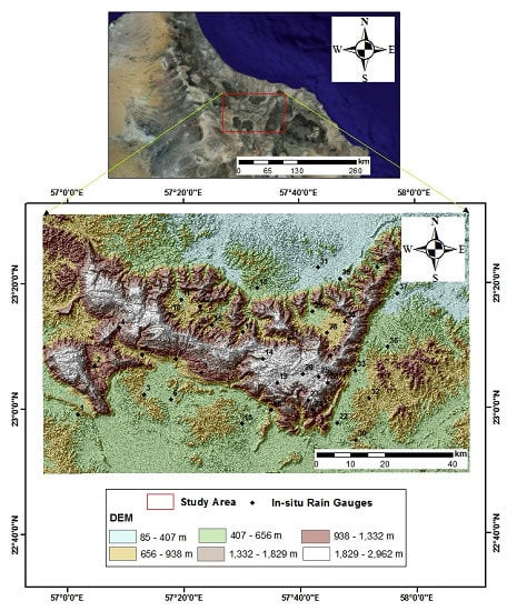
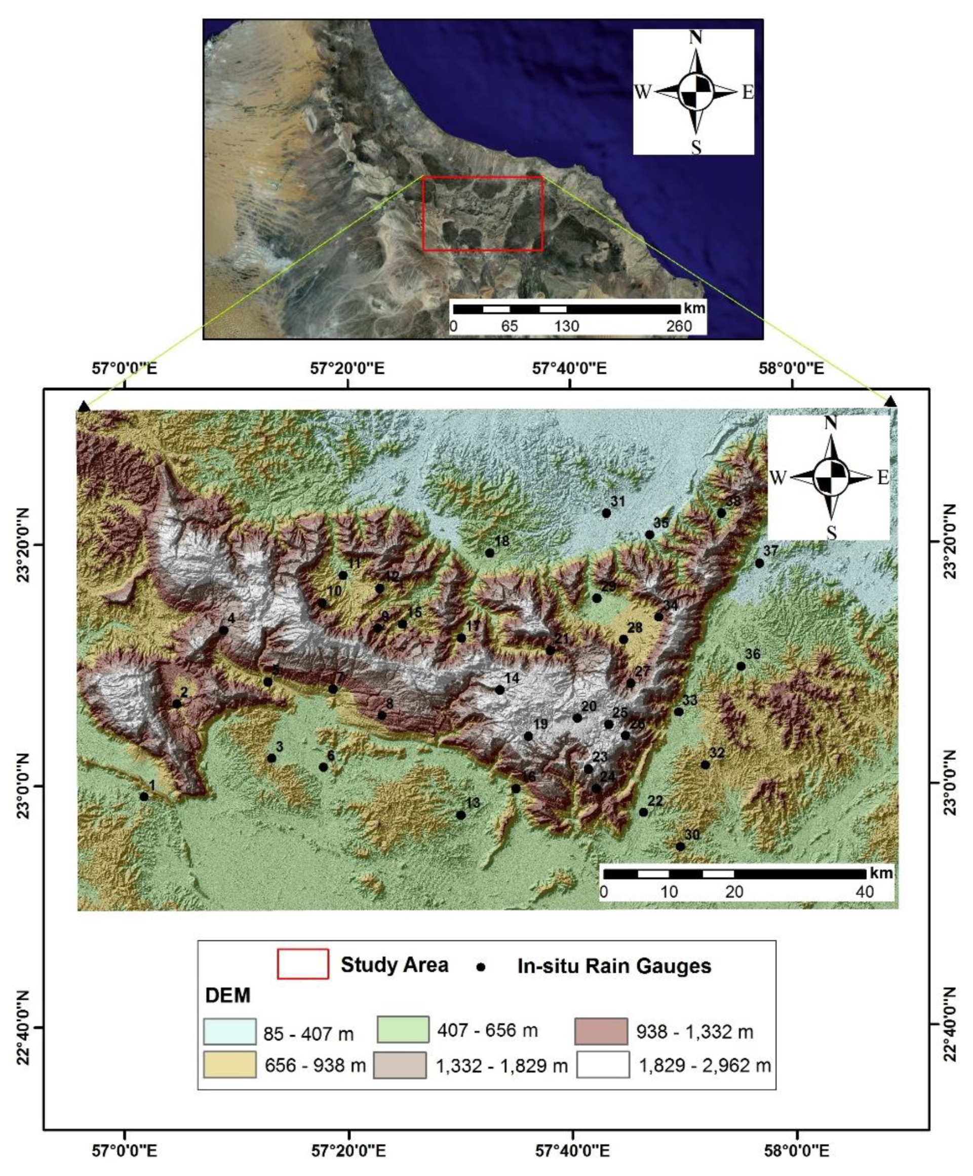
In the Sultanate of Oman (i.e., our proposed study area), water resources are scarce [24]. The primary source of surface and sub-surface water is the rainfall, and complex mountains (400 m–3000 m above sea level [25]) act as water towers [26]. The spatiotemporal performance of GPM and GSMaP estimates has not been studied over arid areas performance of 5 quasi-global GSPEs over an arid environment using in-situ rain gauge measurements as benchmarks. The current paper introduces the first detailed daily and sub-daily assessment of GSPEs over the Arabian Peninsula. With an emphasis on the latency time aspect of these GSPEs, the ultimate objective of this research was to assess their performance per entire ground stations in relationship to different rainfall intensity classes. Because GSPEs have mostly global or quasi-global orientations, the performance of these products is expected to vary from one location to the other. Therefore, it is mandatory to assess the performances of GSPEs using the local in-situ rain gauge datasets before they can be utilized with high confidence in different environmental applications over a specific study area. Such evaluation and inter-comparison can also help to determine the most accurate and appropriate GSPEs among various alternatives.

2. Study Area and Datasets

2.1. Study Area

Our study area, i.e., the Sultanate of Oman is located along the south-eastern coast of the Arabian Peninsula in western Asia. It covers an area of approximately 309,814 km2 [27]. It can be divided geographically into three distinct parts: desert (75%), mountainous area (15%), and coastal zone and alluvial plains (5%). The current study was carried out at the foothill of the Al-Jabal Al-Akhdar chain at Ad Dakhiliyah Governorate, the Sultanate of Oman (Figure 1). It is characterized by the arid climate with little precipitation over the whole year. It is highly variable and fluctuated with an average annual rainfall of more than 300 mm in the northern Oman mountains [28]. In fact, there are four main mechanisms that help generate rainfall in Oman [24,28,29,30], i.e., (i) convective rainstorms that often occur during the summer and may reoccur at any time of the year, (ii) cold frontal troughs that originate over the Atlantic Ocean or the Mediterranean Sea and prevail throughout winter and early spring, (iii) onshore monsoon currents that induce a complex regional circulation from June to September and usually come in the form of drizzle over the southern Oman (Dhofar), and (iv) tropical cyclones that move from the Arabian Sea-side to generate extreme rainfall and can reoccur once in every five years in Dhofar and about once in every ten years over Muscat coastal regions.

2.2. The In-Situ Gauge Measurements

In this study, we used three different precipitation-related datasets: (i) GPM-IMERG, (ii) GSMaP, and (iii) in-situ gauge data. These datasets are briefly described in the following sub-sections.

2.2.1. GPM-IMERG Estimates

The GPM is a constellation of satellite platforms operated by the National Aeronautics and Space Administration (NASA) and the Japan Aerospace Exploration Agency (JAXA) in cooperation with other international space agencies [32]. This system provides precipitation measurements in near-real time (NRT) within 3 hours of observation to enhance our understanding of Earth’s energy and the water cycle. It consists of two integrated instruments, i.e., the GPM Microwave Imager (GMI) captures precipitation intensities and horizontal patterns, and the Dual-frequency Precipitation Radar (DPR) to produce a 3D structure of precipitating particles. It generates Integrated Multi-satellite Retrievals for GPM (IMERG) products by merging and interpolating of: (i) all satellite passive microwave precipitation estimates in the GPM constellation, (ii) microwave calibrated IR satellite measurements, (iii) rainfall gauge records, and (iv) other precipitation products of different sensors at fine spatial and temporal resolutions [32]. The involved methods for developing these IMERG products can be summarized in the following steps as described in [32]: (i) creating a linear interpolation between the LEO-PMW estimates and the GEO-IR-based feature motion, (ii) applying Kalman filter to process the GEO-IR precipitation when the LEO-PMW are too scattered, (iii) implementing satellite sounding-based algorithms at the high latitudes to overcome the shortcomings of the usual PMW imager channels, and (iv) utilizing the precipitation gauge networks to correct the bias of the satellite measurements and produce reliable regionalization. The system runs several times for every observation time to generate products of 0.1° and 30 minutes of spatial and temporal resolution, respectively. There are three IMERG products [33,34]: (i) the NRT IMERG-E run provides quick estimates after 4 h of observations, (ii) the IMERG-L run yields better estimates as more data arrives after 12 h of observations, and (iii) the IMERG-F research-grade that used the monthly in-situ gauge estimates for validation purposes, and has latency time of 3.5 months. The IMERG V04 algorithms use the Goddard Profiling Algorithm (GPROF 2014) to measure the precipitation estimates from all PMW sensors onboard GPM satellites, which represents an improvement compared with GPROF 2010 of the TRMM-TMPA products [32].

2.2.2. GSMaP Estimates

GSMaP is a blended Microwave-IR product and has been developed in Japan for the GPM mission. Processing and distributing global rainfall data on an NRT basis by merging multi-satellite data. It is an hourly product at a 0.1° × 0.1° latitude/longitude grid. The prototype version has been in operation in JAXA since 2006 data, and the GPM-GSMaP products were released in September 2014. A new version of GSMaP (V06) was released on 17 January 2017. Based on launching the GPM mission, the GSMaP project developed a corresponding GPM-era precipitation retrieval algorithm (GPM-GSMaP version 06) by adding information from GPM Core GMI. The GSMaP algorithm generates precipitation estimates according to following steps as described in [35,36,37]: (i) calculating the rainfall rate from PMW sensors, (ii) then propagating rainfall affected area using forward and backward morphing technique, and (iii) finally, refining the estimated data based on infrared brightness temperature using Kalman filter approach. The GSMaP-G is an error-corrected GSMaP product, which is based on GSMaP-MVK (i.e., a pure satellite-based GSMaP product without gauge correction) and adjusted by the CPC unified gauge-based analysis of global daily precipitation data analysis. In this study, we used “GSMaP-G” to stand for GSMaP-Gauge adjusted data, and “GSMaP-S” to denote GSMaP-MVK. More details about GSMaP algorithms, validation, and products can be obtained from [35,36,37].

2.2.3. Rain Gauge Data

In total, the rain measurements from 38 in-situ gauges were collected by the Ministry of Regional Municipalities and Water Resources, the Sultanate of Oman, over the period from March 2014 to October 2016. These in-situ rain gauge data were converted to a spatial vector data structure and georeferenced to the projection system of the GSPEs. Besides, the GSPEs were adjusted to match with the Omani day, which starts 4 h ahead of Coordinated Universal Time/Greenwich Mean Time (UTC/GMT) (i.e., UTC/GMT + 4 h). To compare the GSPEs with the corresponding ground rain records at daily and sub-daily temporal scales, we aggregated the five products of half-hourly, i.e., HH IMERG and hourly GSMaP into daily and sub-daily datasets every 6 h ranging from 00.00 UTC to 24.00 UTC and details can be found in [38].

3. Methods

Figure 2 demonstrates our proposed method in the form of a schematic diagram. It consists of two distinct components: (i) data preparation, and (ii) statistical comparison processes (i.e., continuous and categorical metrics) for daily and sub-daily GSPEs based on the entire in-situ rain gauges’ measurements at different rainfall intensities and thresholds.

3.1. Data Preparation

Llasat [39] stated that there was no generic schema for classifying the rainfall intensity into different categories as they could significantly vary from one country to another. The analysis of in-situ rainfall measurements for the period from 1997 to 2003 over Al-Jabal Al Akhdar toward Ad Dakhiliyah Governorate (Nizwa, Bahla, and Al Hamra cities), Sultanate of Oman revealed that the intensity of rainfall less than 10 mm/day constituted 66-95% of the total rainfall amount, while rainfall of at least 50 mm/day was erratic [24]. Therefore, we selected certain accumulated rainfall intervals (i.e., 0.0–2.5 mm, 2.5–10 mm, 10–50 mm, greater than 50 mm) to evaluate the GSPEs, per different sub-daily and daily temporal resolutions, using the in-situ rain gauges’ measurements. The three runs of the HH IMERG datasets were originally stored in a native complex Hierarchical Data Format (HDF5). The HDF5 is a unique open-source, cross-platform technology for data storage of scientific and descriptive metadata in an organized hierarchy. The IMERG V04 runs were downloaded from the Mirador web tool of NASA Goddard Earth Sciences Data and Information Services Center (GES DISC) for the period from March 2014 to October 2016. The downloaded data were converted to the GeoTIFF data format with subsequent extraction of the calibrated precipitation datasets. The IMERG products were projected to the Geographic Coordinate System (GCS), WGS 1984. The next step was to correct the orientation of the grids by rotating the images through a 90° counter-clockwise, then the corrected georeferenced longitude and latitude values were defined. The point rain gauges were transferred into the same projected coordinate system of the IMERG data. The daily precipitation estimates were calculated by summing the 48 HH precipitation estimates for each day and dividing them by two. The HH IMERG data were divided by two to convert the unit of measurements into mm/hour. The precipitation estimates in successive two HH periods (Xnmm/hh, Xn+1mm/hh) were converted into hourly precipitation estimates (Xmm/h) based on the following mathematical relationship:
X mm / h =   [ Xn mm / hh +   ( Xn + 1 mm / hh ) ] / 2
The GSMaP datasets were available in a CSV file format that contained latitudes, longitudes, and rainfall values. To convert these data into GeoTIFF format, the maximum and minimum values of the longitudes and latitudes were defined. Then, based on determining the full spatial extent of the GSMaP data, the grids were generated, and the pixels were filled iteratively by the precipitation values. The images were then converted to GeoTIFF format and projected to the GCS, WGS 1984.
In order to perform the comparison between the five GSPEs and in-situ gauge measurements, the IMERG and GSMaP raster datasets were converted to vector points that represented the centroid of each pixel. The gauge points were overlaid the IMERG grids, and the nearest neighbor pixel value to each ground station were extracted into matrix of the points’ values (i.e., as columns) (e.g., [20]) using the nearest neighbor approach (i.e., the closest center of the correspondent GSPEs’ grid points were selected). The nearest neighbor could be used to search for k nearest neighbors, or neighbors within some distance (or both). The maximum distance between the center of the GSPEs’ grids and the in-situ gauges was approximately five km (i.e., below the spatial resolution of the GSPEs). This approach is used frequently in evaluating the performance of the GSPEs to ensure using the original retrievals of each satellite estimate [20,40]. The corresponding rainfall event from GSMaP and IMERG grids, and in-situ point measurements were extracted to compute the statistical comparison measures. Ground stations’ records were spatially joined with the closest centroid of the GSPEs’ grids. The results from these spatial joins were used to identify ‘hits’ and ‘misses’.
The in-situ rain measurements and the corresponding GSPEs were aggregated into sub-daily and daily products every 6 h from 00.00 UTC to 24.00 UTC (i.e., from 00.00 to 06.00 UTC, 06.00 to 12.00 UTC, 12.00 to 18.00 UTC, and 18.00 to 24.00 UTC) per all involved gauges in the evaluation. These accumulated products were initially compared per the total rainfall intensity per all in-situ gauges. In addition, in order to gain in-depth information about the performance of GSPEs, we also evaluated them using in-situ rain gauges measurements at different rain intensity intervals (i.e., 0.00–2.5 mm, 2.5–10 mm, 10–50 mm, greater than 50 mm), and at different rainfall initiation thresholds (0.00 mm, 2.5 mm, and 10 mm).

3.2. Statistical Comparison Procedures

In general, statistical evaluation of the performance of GSPEs could be carried out based on the continuous difference (Table 1) and categorical methods (Table 2 and Table 3). In this case, sub-daily and daily cumulative precipitation estimates were used. These assessments were carried out based on different rainfall intensities, as well as different thresholds to differentiate rain and no rain events.

3.2.1. Continuous Statistical Metrics

The continuous difference methods (see Table 1) were mainly directed toward measuring the difference between GSPEs and the corresponding in-situ rain gauges. Numerous statistical difference methods have been reported by various researchers (e.g., [1,16,17,20,41]) to evaluate the performance of different GSPEs. Both root mean square error (RMSE) and mean absolute difference (MAD) measure the average error magnitude, but RMSE provides greater weights to the more substantial errors than the MAD. MD also determines the difference between two products. In the case of using observation data (i.e., reference in-situ gauges’ measurements) are utilized for assessing the performance of the GSPEs, MD is corresponding to the bias. The unconditional bias (UB) is the ratio between the GSPE and in-situ rainfall measurements. Perfect satellite precipitation estimation results in a UB of unity. Overestimation leads to values higher than unity, while underestimation causes values less than unity.

3.2.2. Categorical Indices

The categorical indicators were determined using a 2 by 2 contingency table (Table 2). Precipitation is collected as discrete observable estimates, so there are four possible combinations (Table 3), where ‘H’ is hit (i.e., number of pixels that both of satellite and gauge data simultaneously detected the rainfall at the same location), ‘F’ stands for false alarm (i.e., number of pixels that are recorded by satellite product as rainfall but not by the in-situ gauge), ‘M’ is missed (i.e., number of pixels that are reported as rainfall by the ground gauge but not by the satellite sensor), and ‘X’ refers to ‘null’ or correct negatives (i.e., the number of pixels that are not recognized as rainfall for both satellite data and ground gauge). The possible forms of the categorical statistics [42] are the probability of detection (POD), critical success index (CSI), false alarm ratio (FAR), and frequency bias (FBI) (Table 3). The POD is defined as how often the satellite product successfully estimates the rainfall. IF the POD is equal to 1, this means that the satellite product correctly detects all the rainy pixels compared to the in-situ gauge data. CSI defines the fraction of rain events correctly captured by the satellite sensor. The FAR specifies how often the satellite data detects rainfall when rain does not actually fall to the ground. The FBI explains the ratio of total satellite rainfall alarms to gauges’ fall alarms. FBI is the ratio between predicted and observed rain events [43]. An ideal FBI value is 1, and it can occur if the frequencies of false alarms and missed rainfall events are equal [44,45]. More details about the categorical classification for GSPEs could be found in [40].

4. Results

In this section, we computed the results based on comparing sub-daily and daily gauge measurements with the corresponding GSPEs, at different rainfall intensity classes (except greater than 50 mm) and thresholds, using traditional continuous and categorical statistical metrics. The rationale of excluding the ‘greater than 50 mm’ intensity class was due to the fact that such events were not commonly occurred (i.e., only 14 events) within the study period of interest.

4.1. Daily Analysis Utilizing Traditional Statistical Metrics per Entire Ground Rain Gauges

The evaluation of the daily 5 GSPEs against 38 ground rain gauges has been carried out based on days with only observed rainfall values (Table 4). The number of events captured by both GSMaP products was higher than those recorded by the different GPM-IMERG runs. The MD and UB metrics indicated if the GSPEs under- or over-valued the in-situ rain gauge measurements. At the daily accumulated rainfall intensity, the IMERG-L showed the lowest underestimation rate with MD of −0.43 mm/day and UB closed to unity, i.e., 0.92 (Table 4). The 5 GSPEs slightly overestimated the light rainfall of intensity of less than 2.5 mm. The IMERG-F reported the lowest overestimation and followed by GSMaP-G and GSMaP-S. The UB and MD metrics were consistent in the case of IMERG-F, GSMaP-G, and GSMaP-S with values of 1.75, 1.84, and 2.08 and 0.64 mm/day, 0.71 mm/day, and 0.92 mm/day, respectively (Table 4). The IMERG-L and IMERG-E, respectively, had the best performance with reporting the lowest underrated values of moderate to heavy ground rainfall observations. They slightly, moderately, and massively undervalued in-situ measurements at rainfall intensity classes of 2.5–10 mm/day, 10–50 mm/day, and greater than 50 mm/day, respectively (Table 4).
Also, the GSMaP-G, GSMaP-S, and IMERG-F yielded the best (i.e., lowest) values of RMSE and MAE at the accumulated rainfall intensity per day (Table 4). At the first three rainfall intensity classes in ascending order, the GSMaP-G kept providing lower values of RMSE and MAE than other GSPEs (Table 4). There were some exceptions where the IMERG-F and IMERG-E ranked first at rainfall intensity classes of 10–50 mm and greater than 50 mm, respectively.

4.2. Sub-Daily Analysis Utilizing Traditional Statistical Metrics per Entire Ground Gauges

In terms of MD and UB metrics, it was found that the GSMaP-G, IMERG-E, and GSMaP-S tended to underestimate the ground rain measurements in ascending order at the accumulated total rainfall intensity per 6 h (Table 5). The computed MD and UB values were close to each other among 5 GSPEs with difference ranges of 0.58 mm/6 h and 0.24, respectively. Using the same metrics per 12 h, the 5 GSPEs kept underestimating the in-situ rain records, where IMERG-L yielded the best MD and UB scores, i.e., −1.59 mm/12 h and 0.58, and followed by GSMaP-S and IMERG-E. Moving toward the accumulated rain per 18 h, it was found that IMERG-L, IMERG-E, and GSMaP-S outperformed the other two GSPEs by reporting the lowest MD values and the closest UB values to the unity (Table 5).
The MAD and RMSE values increased with the rise of accumulated hours from 6 to 18 h (Table 5). The GSMaP-G showed the best performance with reporting lowest RMSE and MAD values of 4.38 mm/6 h, 7.55 mm/12 h, and 8.87 mm/h and 1.88 mm/6 h, 3.3 mm/12 h, and 4.55 mm/18 h, respectively. The IMERG-F showed similar performance to GSMaP-G at 12 and 18 h. GSMaP-S had the lowest performance per 6 h, while IMERG-L outperformed by other GSPEs per 12 and 18 h (Table 5).
Table 6 shows that the 5 GSPEs inclined to overestimate the sub-daily ground rain measurements at a rain intensity of 0.0–2.5 mm. The MD and UB values ranged from 0.00–0.32 mm and 0.24–0.48, respectively, for the accumulated rain per 6 h, where 5 GSPEs tended to overestimate the in-situ rain measurements except for the IMERG-F slightly. GSMaP-G showed the highest performance per 6 h, and IMERG-F ranked first pr 12 and 18 h with reporting best MD and UB scores. For the other GSPEs, the IMERG-E, GSMaP-S, and IMERG-L ranked in descending order with MD and UB values of 0.21 mm/12 h, 0.51 mm/12 h, and 0.59 mm/12 h and 1.28, 1.69, and 1.79, respectively (Table 6). The same rank was achieved at a temporal resolution of 18 h, except that the GSMaP-G outperformed the IMERG-E. The scores of RMSE and MAD were close to each other at different sub-daily time scales except for the extreme RMSE reported at a temporal resolution of 18 h by the IMERG-L, i.e., 10.01 mm/18 h and IMERG-F, i.e., 8.32 mm/18 h (Table 6). The GSMaP-G and IMERG-F alternately had the best performance at different sub-daily time scales.
Within accumulated rainfall intensity ranged from 2.5–10 mm, the GSMaP-G was found to be the best depending among different intervals of computations (Table 7). GSMaP-G was the best performer for 8 out of 12 times, i.e., (i) −2.54 mm, 3.74 mm, 4.38 mm, and 0.54 for MD, MAD, RMSE, and UB, respectively, per 6 h; and (ii) approximately 4.16 mm, 4.86 mm for MAD and RMSE, respectively, per 12 and 18 h. In terms of MD and UB metrics, the 5 GSPEs tended to underestimate moderately the in-situ rain measurements (Table 7). The IMERG-L demonstrated the closest matching with in-situ rainfall measurements with reporting lowest MD values, i.e., −2.65 mm and −0.57 mm, and UB scores, i.e., 0.52 and 0.89 per 12 and 18 h, respectively.
In terms of MAD and RMSE, the GSMaP-G and IMERG-F had the highest performance and followed by the GSMaP-S, IMERG-E, and IMERG-L at the three temporal resolutions. There was an exception at a temporal resolution of 6 h where IMERG-L and GSMaP-S were ranked second and fifth in the performance order, respectively.
Within a rainfall intensity between 10 mm and 50 mm (Table 8), the computed MD and UB values were much larger than those estimated at a rainfall intensity of 2.5–10 mm (Table 7). These values can be interpreted by the possible occurrence of heavy rainfall events that were captured by the in-situ gauges while heavily undervalued by the GSPEs. The GSMaP-G reported the minimum MD values, i.e., −14.74 and −3.64 mm at temporal resolutions of 6 and 12 h, and the IMERG-L, i.e., −8.42 mm when evaluating the accumulated rainfall per 18 h (Table 8). The UB and MD values were consistent, where the UB scores also proved that IMERG-F heavily underestimated the ground rain measurements at temporal resolutions of 6 and 12 h, and GSMaP-G at a time interval of 18 h (Table 8).
The computed MAD and RMSE values at a rainfall intensity of 10–50 mm (Table 8) were approximately three times more than those estimated at rainfall intensity of 2.5–10 mm (Table 7). The reported MAD and RMSE values at a temporal resolution of 6 h were larger than those computed at the accumulated rainfall per 12 h and 18 h. This could be interpreted by the extreme rainfall intensities at the early night times (i.e., 00.00 to 06:00 UTC/GMT). The MAD and RMSE values were matched at a time interval of 6 h since the GSMaP-G had the best performance and followed by the IMERG-E, IMERG-L, GSMaP-S, and IMERG-F in ascending order. On the contrary, there was a different performance, where GSMaP-G ranked first and was followed by GSMaP-S, IMERG-F, IMERG-L, and IMERG-E at a temporal resolution of 12 h. Furthermore, the smallest MAD and RMSE values were reported by the IMERG-F, i.e., 13.8 mm and 15.77 mm, and GSMaP-G, i.e., 14.24 mm and 16.2 mm, respectively, at 18 h. (Table 8).

4.3. Daily Analysis Utilizing Categorical Metrics per Entire Ground Gauges

In order to calculate the categorical metrics, each day over the whole period of study was considered whether the observations from either both in-situ gauges and GSPEs were available or not. Figure 3 shows that the GSMaP-G, IMERG-L, and a GSMaP-S had the highest POD with a value of approximately 0.7 and 0.4 at the initialization thresholds of 0.00 and 2.5 mm/day, respectively. The IMERG-L and GSMaP-S kept providing most top POD scores, and IMERG-E showed a significant improvement at an initialization threshold of 10 mm. The POD decreased with the rise of rainfall initiation threshold from 0.00 to 10 mm. Low POD might be interpreted by the missed precipitation due to possible occurrences of snow coverage on the top of Al-Jabal Al Khader, and by the incapability of capturing warm rain processes or short-lived convective storms [40], where these conditions prevailed along the Gulf of Oman. The GSMAP-S and GSMaP-G reported the highest CSI values at the three rainfall thresholds. The other GSPEs had close CSI values to those reported by the GSMAP-S and GSMaP-G with a maximum difference of 0.1 in the case of IMERG-F (Figure 3).
At the initialization threshold of 0 mm/day, the GSMaP-S had the best performance with the lowest FAR, i.e., 0.64, while the other GSPEs had closer FAR values with a difference of 0.06 (Figure 3). GSMaP-S again had the lowest FAR, i.e., 0.61 at a rain threshold of 2.5 mm, while the IMERG-L ranked last among the 5 GSPEs with FAR of 0.71. The IMERG-F reported the lowest FAR and was followed by GSMaP-G and GSMaP-S by values of 0.57, 0.59, and 0.63, respectively, at a rain threshold of 10 mm/day. The FBI and FAR scores were consistent, where GSMaP-S reported the best values, i.e., 2.07, 1.06, and at rain thresholds of 0.00 and 2.5 mm/day, respectively. With the increase of the rain threshold value to 10 mm/day, the IMERG-F and GSMaP-G had the best FAR, i.e., approximately 1.

4.4. Sub-Daily Analysis Utilizing Categorical Metrics per Entire Ground Gauges

GSMaP-G generally showed the best performance since it came in the first place among other GSPEs at temporal resolutions of 6 h and 12 h, and third at 18 h with POD values of 0.57, 0.66, and 0.64, respectively (Figure 4). The GSMaP-S came in the second rank with reporting POD values of 0.65 and 0.75 at the sub-daily time scales of 12 and 18 h; however, it ranked last in at 6 h (Figure 4). High POD might be interpreted by the domination of convective storms [38]. IMERG-L and IMERG-F reported approximately similar POD values that were lower than those computed from GSMaP-G and GSMaP-S at different latency times (Figure 4). CSI of GSMaP S seems to be better than other GSPEs at daily time scales of 6, 12, and 18 h (Figure 4) by values of 0.19, 0.24, and 0.32, respectively.
In general, the GSMaP-S mostly recorded the lowest FAR and FBI values at different temporal resolutions. The GSMaP-G had the worst FAR and FBA at 6 and 12 h. Its performance improved 18 h, where it ranked first with reporting the lowest FAR and FBI, i.e., 0.67 and 1.97, respectively. The IMERG-L and IMERG-E yielded the highest FAR and FBI scores at the three sub-daily time scales (Figure 4).
Figure 5 shows the results of evaluating 5 GSPEs using the categorical indices at a light rainfall intensity from 0.00–2.5 mm. Both GSMaP products showed the highest POD and CSI values at different sub-daily and daily times scales. They have equal POD values, i.e., 0.65, at a daily time scale, while GSMaP-G outperformed the GSMaP-S by differences of 0.19 and 0.04 at the time latency of 6 and 12 h, respectively. At a time-scale of 18 h, GSMaP-S had a higher POD value than GSMap-G. GSMaP-S slightly outperformed GSMaP-G with reporting higher CSI scores at 6, 12, 18, and 24 h. The IMERG products had the lowest performance with reporting approximately equal POD and CSI scores with a slight improvement in the case of IMERG-F and IMERG-L at different sub-daily and daily scales.
The GSMaP-S had the best performance with the lowest reported FAR values of 0.79, 0.83, 0.78, and 0.78 at time scales of 6, 12, 18, and 24 h, respectively (Figure 5). The GSMaP-G outperformed the other three IMERG products; however, the reported FAR sores from these 4 GSPEs were very close with minimum values of 0.92, 0.87, 0.8, and 0.83 at time latency of 6, 12, 18, and 24 h, respectively (Figure 5). The FBI values also supported that the GSMaP-S had the highest performance among other GSPEs at different time scales. The other GSPEs had fluctuated performance at different times scales. The IMERG-E reported the lowest FBI values except at a time scale of 18 h, where GSMaP-S yielded the lowest value, i.e., 2.94 (Figure 5). IMERG-F and IMERG-L showed the weakest performance with respect to FBI values, except at a temporal resolution of 6 h (Figure 5).

5. Discussion

The use of the daily in-situ rainfall gauges as benchmarks to evaluate the performance of the GSPEs has been less documented by previous studies over the arid Arabian Peninsula. Over entire Saudi Arabia, Mahmoud et al. [21] evaluated the three GPM-IMERG runs using 1455 records from 189 in-situ rain gauges during the period October 2015–April 2016. Utilizing the entire ground stations, the reported RMSE and MAD values ranged from 10 mm/day to greater than 40 mm/day. The reported categorical performance metrics such as POD and CSI were greater than 0.6, 0.7, and 0.9 in case of the early, late, and final IMERG products, respectively. The MAE values of the IMERG-E run ranged from 10–25 mm/day, while they showed slight improvement in the case of IMERG-L. The IMERG-F yielded the lowest MAD with values less than 10 mm/day. The reported RMSE values ranged from 10 mm/day to greater than 30 mm/day in the case of IMERG-E, and they provided considerable improvement with reduced RMSE values from 40 mm/day to 20 mm/day over some regions. The IMERG-F mostly yielded RMSE values less than 10 mm/day, with few exceptions at some regions where they reached 30 mm/day. Based on the individual stations, the estimated RMSE, MD, and MAD ranged from 15 mm/day to greater than 55 mm/day, −20 mm/day to greater than 20 mm/day, and 5 mm/day to greater than 40 mm/day, respectively. The reported categorical performance metrics such as POD and CSI values ranged from less than 0.5 to greater than 0.85. The IMERG-F showed a higher accuracy over the other two IMERG runs that had fluctuated performance between over- and under-estimation of the in-situ gauge measurements over the different regions of Saudi Arabia.
In 2019, Mahmoud et al. [22] evaluated the accuracy of the three GPM-IMERG products utilizing 1600 in-situ measurements recorded from 81 rain gauges from January 2015–December 2017 over the entire area of UAE. The IMERG-F reported the highest accuracy and lowest estimation error compared to other IMERG products. The late run showed a slight improvement over the early product. The regional evaluation of the early, late, and final IMERG products reported POD values that ranged from 0.68–0.8, 0.7–greater than 0.8, and greater than 0.85, respectively. On the basis of evaluating the individual stations, an overall high detection accuracy with POD greater than 0.75 was recorded. Based on the evaluation of the IMERG products using the entire ground stations, the early and late runs showed MAD and RMSE values that generally ranged from 10 mm/day to greater than 15 mm/day, and 15 mm/day to 30 mm/day, respectively. The late run showed a higher estimation error than that observed in the early product with an average increment of 15%. The IMERG-F product reported difference error lower than the other IMERG product with MAD and RMSE values that ranged from 9–11 mm/day and from less than 15–21 mm/day. The individual station-based assessment showed similar results to the regional assessment, but the RMSE reached more than 40 mm/day in some locations.
Nashwan et al. [46] validated three GSPEs (IMERG-F V05, GSMaP V07, and Climate Hazards Group InfraRed Precipitation with Stations (CHIRPS)) over Egypt during the period from March 2014–May 2018. They used 670 rainfall events recorded by 29 in-situ meteorological stations that collected by the US National Climate Data Center Global Summary of Days (GSOD). Although the three GSPEs are gauge-corrected, they did not show consistent performance. Therefore, no single product can be named as the best/worst performing product in Egypt. Without classifying the rainfall intensity, the CHIRPS ranked first with the lowest estimation error, i.e., median RMSE = 2 mm/day. The median values of RMSE reported by the IMERG-F and GSMaP-G were found to be close to that provided by CHIRPS. For the light rainfall intensity class, the GSMaP-G and CHIRPS generally demonstrated similar median RMSE values, i.e., 1.03 mm/day. The same results were reported from the low-moderate rainfall intensity class, but CHIRPS showed a slightly higher median RMSE value, i.e., 2.82 mm/day, than the GSMaP_G. Furthermore, GSMaP-G recorded also the lowest median RMSE at the heavy rainfall intensity class. The three GSPEs reported weak performance for the heavy rainfall class with the highest median RMSE value, i.e., 51 mm/day. The GSMaP-G and IMERG-F similarly captured the spatial distribution of the rainfall, but the GSMaP-G was more consistent with the in-situ observations than the IMERG-F run. In general, the lack of detailed ground rainfall records may contribute significantly to the unsatisfactory performance of the three GSPEs. The accurate detection of rainfall using the GSPEs over the arid climate, particularly the deserts of hot climate is still challenging and open for further studies. Nashwan et al. [46] stated that their research was constrained by the lack of dense in-situ rainfall measurements. More daily and sub-daily ground gauge records are needed to evaluate the diurnal rainfall cycles of the IMERG-F and GSMaP-G at fine temporal resolutions.
The findings of Nashwan et al. [46] were similar to our results at the daily time scale, but the magnitude of the estimated errors was lower in our case study. Additionally, the previous studies showed that the performance of the different GSPEs was inconsistent with respect to the in-situ gauge measurements. Although this fluctuated performance, our findings agreed with the other authors that GSMaP-G mostly provides the best performance. Additionally, the IMERG-F slightly outperformed the IMERG-E and IMERG-L.
Water was, still, and will be the most influential factor in Earth’s evolution [47]. The need for continuous and long precipitation records of high accuracy and free availability is a frequent problem for the environmental modelers [48]. Reliable rainfall records constitute integral inputs of different environmental models, particularly flood inundation modeling (e.g., [49] and their associated watershed (e.g., [50,51]), runoff (e.g., [52]), groundwater flow and recharge (e.g., [53]), surface and subsurface water pollution (e.g., [54]), soil moisture (e.g., [55]), optimum water management (e.g., [56]), climate prediction and forecasting (e.g., [57], and hazard assessment (e.g., [58]) models. The GSPEs introduce an alternative and promising source of continuous rainfall records for different hydrological and environmental applications, particularly over the arid area [46,59]. There is no perfect rainfall data, but selecting the optimum datasets depend mainly on the purpose of the given application [48]. Additionally, choosing precipitation records depend on the method, spatial, and temporal resolutions [60], which can give the advantage of using GSPEs over the traditional gauge data in various environmental applications.
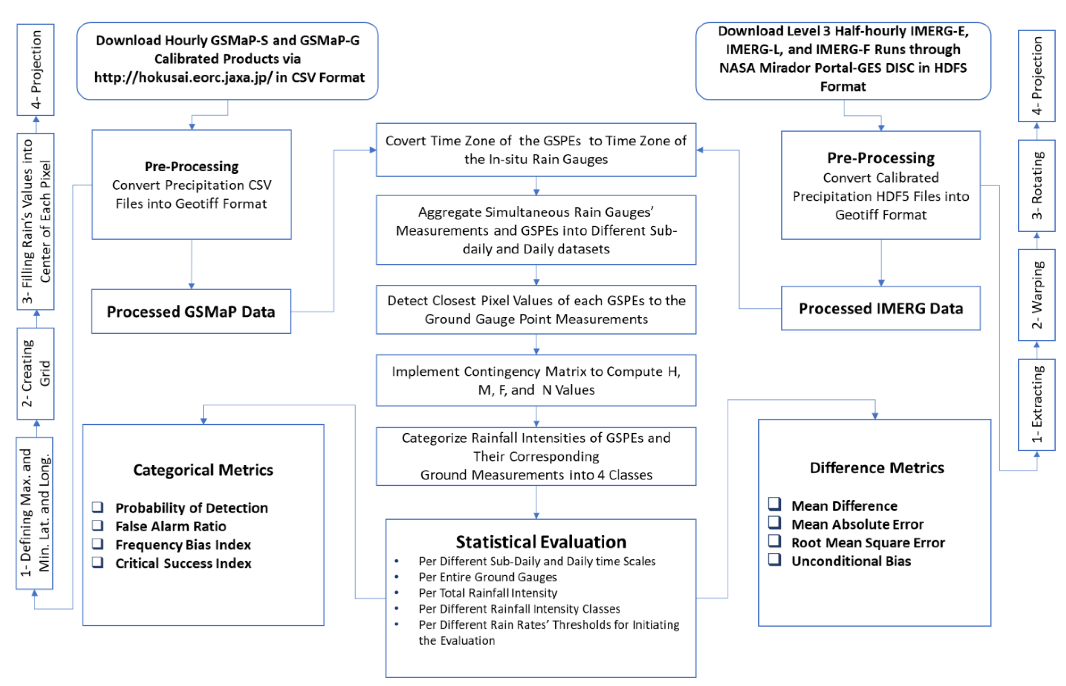
6. Conclusions

This paper presented a detailed statistical evaluation of 5 GSPEs (GEMaP-S, GSMaP-G, IMERG-E, IMERG-L, and IMERG-F). In general, the performance of the 5 GSPEs enhanced with receiving more spaceborne estimates throughout the day. Both GSMaP products reported the best statistical metrics, among other GSPEs, in most of daily and sub-daily comparisons with the in-situ rain gauge measurements. The IMERG-F slightly outperformed the IMERG-L and IMERG-E. However, the early and late IMERG runs gave promising results, particularly they have shorter latency times (i.e., 4 and 12 h, respectively) and uncorrected with gauge information. The availability of these products within shorter times than the other GSPEs can help in different hydrological applications such as monitoring flash flood over fine sub-daily temporal resolutions. Up to our knowledge, there were no previous studies concerning evaluating different GSPEs at sub-daily time scales over this extremely arid area of the world. The assessment of the 5 GSPEs over daily and sub-daily time intervals revealed the following:
The overall performance of the 5 GSPEs in capturing daily rainfall events of the total intensity class was acceptable in comparison with the results reported from previous literature mentioned above in the discussion section. With respect to the error difference between GSPEs and ground gauge records, the GSMaP-G, IMERG-F, and GSMaP-S showed the lowest recorded RMSE and MAD values. In terms of MD and UB metrics, The IMERG-L ranked first with reporting the lowest underestimation values, and IMERG-E and GSMaP-G came in the second and third places, respectively.
  • The 5 GSPEs generally underestimated the in-situ rainfall measurements at different rainfall intensity classes, except for the light rainfall of an intensity less than 2.5 mm/day. With respect to the underestimation of moderate to heavy in-situ rainfall records per daily basis, the IMERG-L ranked first with reporting the lowest underestimation values and followed by IMERG-E and GSMaP-S.
  • The underestimation of ground rainfall measurements per day raised with the increase of the rainfall intensity from less than 2.5 mm/day to greater than 50 mm/day.
  • At both daily and sub-daily time scales, the lowest RMSE and MAD values were mostly demonstrated by GSMaP-G, IMERG-F, and GSMaP-S, respectively. The only exception was at a rainfall intensity greater than 50 mm/day, where IMERG-E and IMERG-L came in the first two places with reporting the lowest recorded RMSE and MAD values.
  • The daily performance of the 5 GSPEs at a rainfall intensity greater than 50 mm was very low, where they heavily underestimated the ground rainfall measurements. This weak performance could be interpreted by the minor amount of reported rainfall events (i.e., 14) for the short period of mid-March 2014 to October 2016, as well as the erratic behavior of rain over the arid areas.
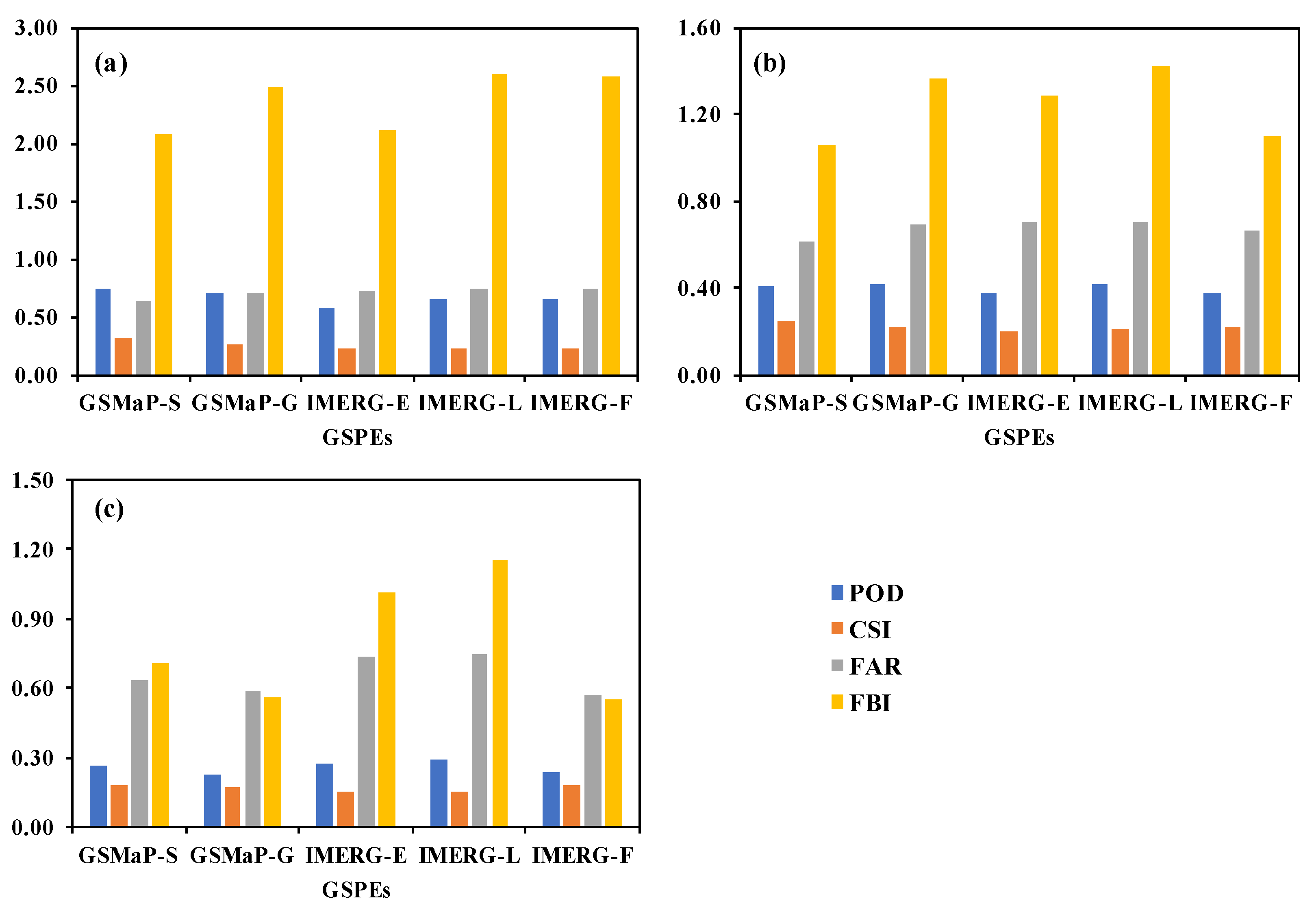
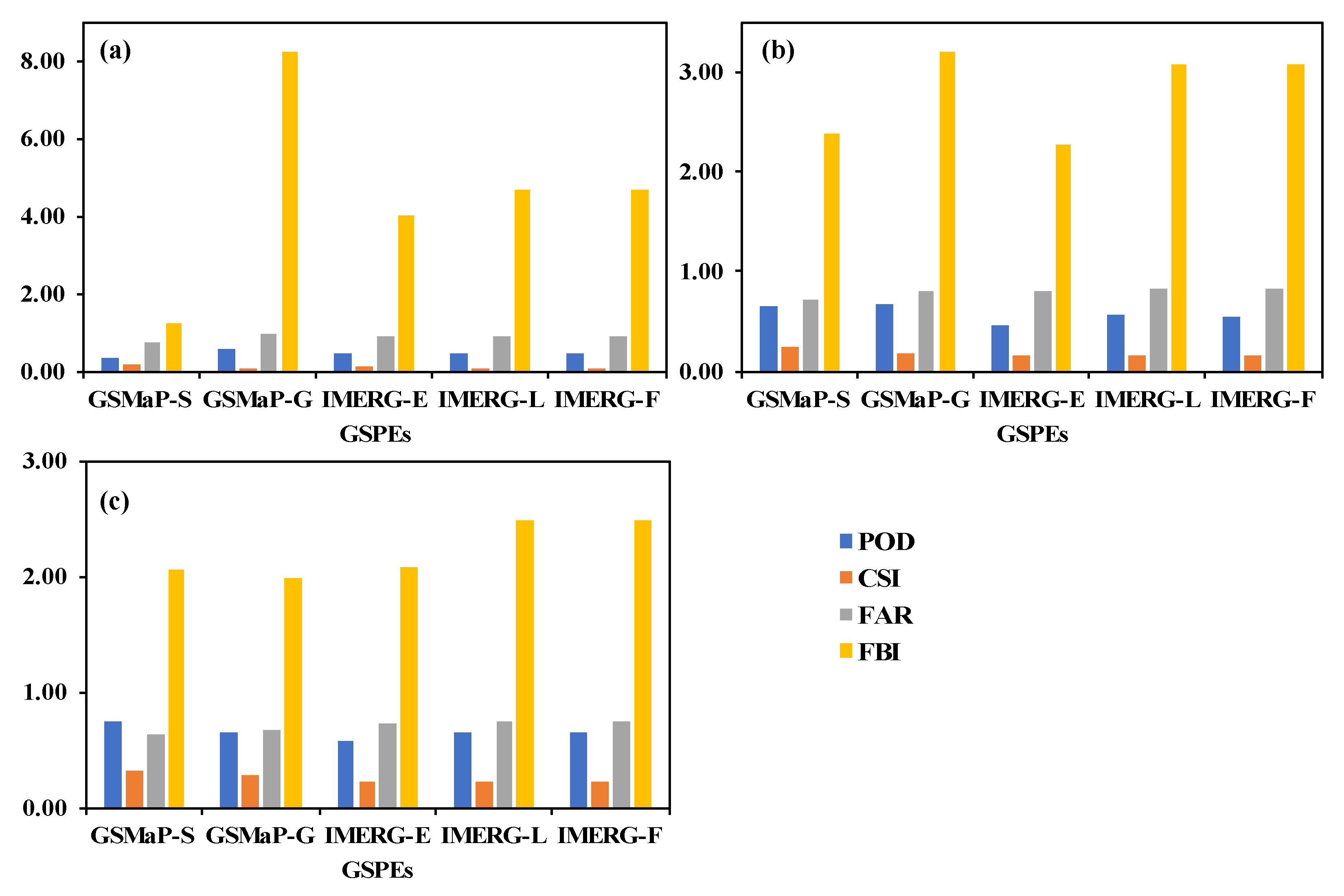
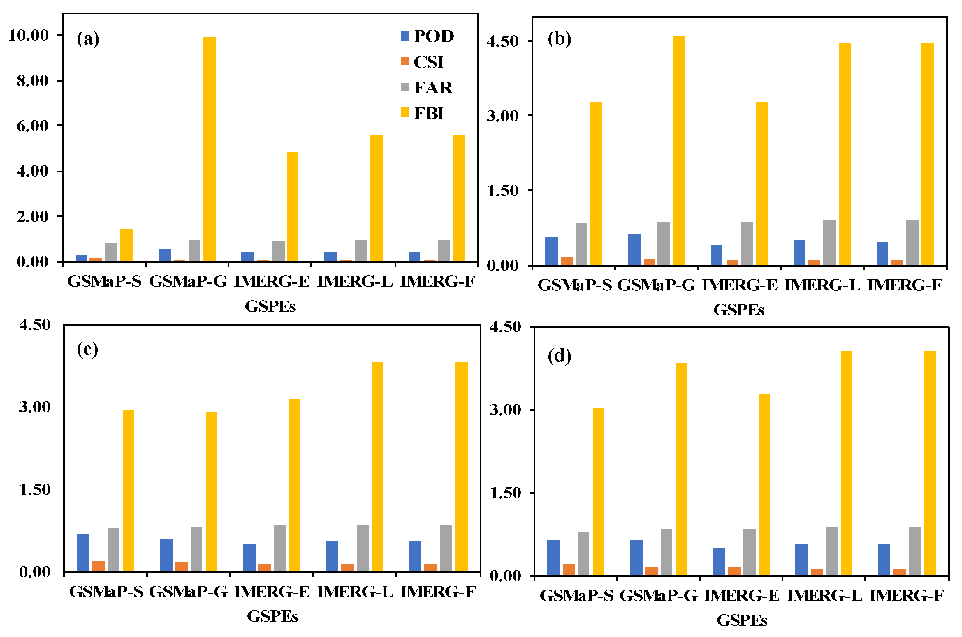
  • For the 5 GSPEs, the POD and CSI values improved, and FAR and FBI measures decreased with the increase of the temporal resolution from 6 to 18 h.
  • The GSMaP-G showed the lowest underestimation degree of the ground rainfall measurements of accumulated rain intensity per 6 h, while IMERG-L outperformed the other GSPEs per 12 and 18 h.
  • At a rainfall intensity of less than 2.5 mm per sub-daily time intervals, the GSMaP-G and IMERG-F closely matched with ground rainfall measurements with reporting the lowest MD, MAD, and RMSE values, as well as UB sores close to unity.
  • Within a rainfall intensity class between 2.5–10 mm/h, GSMaP-G had a good agreement with in-situ rain observations per 6 h, while IMERG-L showed higher matching than the other GSPEs at the time intervals of 12 and 18 h. The GSMaP-G and IMERG-F showed the lowest statistical error differences at the three different temporal resolutions.
  • At a rainfall intensity of 10–50 mm/h, the estimated MD and UB values were much larger than those estimated at the light and moderate rainfall intensity classes. These values could be interpreted by the possible occurrence of heavy rainfall events that were captured by the in-situ gauges while massively undervalued by the GSPEs.
  • GSMaP-G had the closest matching with the ground rain measurements at the early night hours (i.e., 00.00 to 06:00 UTC/GMT). With moving toward the daytime (i.e., 06:00 to 12:00 and 12:00 to 18:00 UTC/GMT), IMERG-F showed the best performance with reporting the lowest MD among other GSPEs. Additionally, the reported error differences during early night times were larger than those computed in the day time.
  • Concerning the accumulated rainfall at a rain threshold of 0.00 mm per different sub-daily time scales, the two GSMaP products kept mostly achieving the top performance on the basis of POD and CSI metrics. GSMaP-S ranked first with reporting lowest FAR and FBI at different time intervals except at 18 h, where it came second after GSMaP-G.
  • With respect to evaluating light rainfall of an intensity of less than 2.5 mm per sub-daily and daily time intervals, the GSMaP products outperformed IMERG runs based on the 4 categorical measures.
  • Based on the achieved findings and with the difficulties in having continuous and reliable rainfall records from in-situ gauge networks, we would recommend that the researchers in the arid areas should pay more attention to use and assess the available GSPEs in their hydrological and water management studies.

Author Contributions

Conceptualization, M.S., A.M., Q.K.H., and N.E.-S..; Formal Analysis, M.S.; Data Curation, M.S.; Writing-Original Draft Preparation, M.S.; Writing-Review & Editing, A.M., Q.K.H., and N.E.-S.; Supervision, Q.K.H., and N.E.-S.; Funding Acquisition, M.S.

Funding

The Ministry of Higher Education and Scientific Research of Egypt, Cultural Affairs and Missions Sector.

Acknowledgments

The authors would like to thank: (i) both NASA and JAXA for providing various types of the satellite precipitation products; and (ii) Ministry of Regional Municipalities and Water Resources, the Sultanate of Oman for providing rain gauge data.

Conflicts of Interest

The authors declare no conflict of interest.

References

  1. Blacutt, L.A.; Herdies, D.L.; De Goncalves, L.G.G.; Vila, D.A.; Andrade, M. Precipitation comparison for the CFSR, MERRA, TRMM3B42 and Combined Scheme datasets in Bolivia. Atmos. Res. 2015, 163, 117–131. [Google Scholar] [CrossRef]
  2. Huffman, G.J.; Bolvin, D.T.; Nelkin, E.J.; Wolff, D.B.; Adler, R.F.; Gu, G.; Hong, Y.; Bowman, K.P.; Stocker, E.F. The TRMM Multisatellite Precipitation Analysis (TMPA): Quasi-Global, Multiyear, Combined-Sensor Precipitation Estimates at Fine Scales. J. Hydrometeorol. 2007, 8, 38–55. [Google Scholar] [CrossRef]
  3. AlHammoud, B.; Claud, C.; Funatsu, B.M.; Béranger, K.; Chaboureau, J.-P. Patterns of Precipitation and Convection Occurrence over the Mediterranean Basin Derived from a Decade of Microwave Satellite Observations. Atmosphere 2014, 5, 370–398. [Google Scholar] [CrossRef]
  4. De Coning, E.; Poolman, E. South African Weather Service operational satellite based precipitation estimation technique: Applications and improvements. Hydrol. Earth Syst. Sci. 2011, 15, 1131–1145. [Google Scholar] [CrossRef]
  5. Bangira, T.; Maathuis, B.H.; Dube, T.; Gara, T.W. Investigating flash floods potential areas using ASCAT and TRMM satellites in the Western Cape Province, South Africa. Geocarto Int. 2015, 30, 1–18. [Google Scholar] [CrossRef]
  6. Germann, U.; Galli, G.; Boscacci, M.; Bolliger, M. Radar precipitation measurement in a mountainous region. Q. J. R. Meteorol. Soc. 2006, 132, 1669–1692. [Google Scholar] [CrossRef]
  7. Hou, A.Y.; Kakar, R.K.; Neeck, S.; Azarbarzin, A.A.; Kummerow, C.D.; Kojima, M.; Oki, R.; Nakamura, K.; Iguchi, T. The Global Precipitation Measurement Mission. Bull. Am. Meteorol. Soc. 2014, 95, 701–722. [Google Scholar] [CrossRef]
  8. Asante, K.O.; Macuacua, R.D.; Artan, G.A.; Lietzow, R.W.; Verdin, J.P. Developing a Flood Monitoring System From Remotely Sensed Data for the Limpopo Basin. IEEE Trans. Geosci. Remote Sens. 2007, 45, 1709–1714. [Google Scholar] [CrossRef]
  9. Gebregiorgis, A.S.; Hossain, F. How well can we estimate error variance of satellite precipitation data around the world? Atmos. Res. 2015, 154, 39–59. [Google Scholar] [CrossRef]
  10. Kidd, C.; Kniveton, D.R.; Todd, M.C.; Bellerby, T.J. Satellite Rainfall Estimation Using Combined Passive Microwave and Infrared Algorithms. J. Hydrometeorol. 2003, 4, 1088–1104. [Google Scholar] [CrossRef]
  11. Tapiador, F.J.; Turk, F.; Petersen, W.; Hou, A.Y.; García-Ortega, E.; Machado, L.A.; Angelis, C.F.; Salio, P.; Kidd, C.; Huffman, G.J.; et al. Global precipitation measurement: Methods, datasets and applications. Atmos. Res. 2012, 104, 70–97. [Google Scholar] [CrossRef]
  12. Michaelides, S.; Levizzani, V.; Anagnostou, E.; Bauer, P.; Kasparis, T.; Lane, J. Precipitation: Measurement, remote sensing, climatology and modeling. Atmos. Res. 2009, 94, 512–533. [Google Scholar] [CrossRef]
  13. Strangeways, I. Improving precipitation measurement. Int. J. Clim. 2004, 24, 1443–1460. [Google Scholar] [CrossRef]
  14. Liechti, T.C.; Matos, J.P.; Boillat, J.-L.; Schleiss, A.J. Comparison and evaluation of satellite derived precipitation products for hydrological modeling of the Zambezi River Basin. Hydrol. Earth Syst. Sci. 2012, 16, 489–500. [Google Scholar] [CrossRef]
  15. Pan, M.; Li, H.; Wood, E. Assessing the skill of satellite-based precipitation estimates in hydrologic applications. Water Resour. Res. 2010, 46. [Google Scholar] [CrossRef]
  16. Zhao, H.; Yang, S.; You, S.; Huang, Y.; Wang, Q.; Zhou, Q. Comprehensive Evaluation of Two Successive V3 and V4 IMERG Final Run Precipitation Products over Mainland China. Remote Sens. 2017, 10, 34. [Google Scholar] [CrossRef]
  17. Su, J.; Lü, H.; Zhu, Y.; Wang, X.; Wei, G. Component Analysis of Errors in Four GPM-Based Precipitation Estimations over Mainland China. Remote Sens. 2018, 10, 1420. [Google Scholar] [CrossRef]
  18. Milewski, A.; Elkadiri, R.; Durham, M. Assessment and Comparison of TMPA Satellite Precipitation Products in Varying Climatic and Topographic Regimes in Morocco. Remote Sens. 2015, 7, 5697–5717. [Google Scholar] [CrossRef]
  19. Satgé, F.; Hussain, Y.; Bonnet, M.-P.; Hussain, B.M.; Martinez-Carvajal, H.; Akhter, G.; Uagoda, R. Benefits of the Successive GPM Based Satellite Precipitation Estimates IMERG–V03, –V04, –V05 and GSMaP–V06, –V07 Over Diverse Geomorphic and Meteorological Regions of Pakistan. Remote Sens. 2018, 10, 1373. [Google Scholar]
  20. Rozante, J.R.; Vila, D.A.; Chiquetto, J.B.; Fernandes, A.D.A.; Alvim, D.S. Evaluation of TRMM/GPM Blended Daily Products over Brazil. Remote Sens. 2018, 10, 882. [Google Scholar] [CrossRef]
  21. Mahmoud, M.T.; Al-Zahrani, M.A.; Sharif, H.O. Assessment of global precipitation measurement satellite products over Saudi Arabia. J. Hydrol. 2018, 559, 1–12. [Google Scholar] [CrossRef]
  22. Mahmoud, M.T.; Hamouda, M.A.; Mohamed, M.M. Spatiotemporal evaluation of the GPM satellite precipitation products over the United Arab Emirates. Atmos. Res. 2019, 219, 200–212. [Google Scholar] [CrossRef]
  23. Wehbe, Y.; Ghebreyesus, D.; Temimi, M.; Milewski, A.; Al Mandous, A. Assessment of the consistency among global precipitation products over the United Arab Emirates. J. Hydrol. Reg. Stud. 2017, 12, 122–135. [Google Scholar] [CrossRef]
  24. Kwarteng, A.Y.; Dorvlo, A.S.; Kumar, G.T.V. Analysis of a 27-year rainfall data (1977-2003) in the Sultanate of Oman. Int. J. Clim. 2009, 29, 605–617. [Google Scholar] [CrossRef]
  25. Al-Kalbani, M.S.; Martin FP, J.C.; Price, M.F. Recent Trends in Temperature and Precipitation in Al Jabal Al Akhdar, Sultanate of Oman, and the Implications for Future Climate Change. J. Earth Sci. Clim. Chang. 2015, 6, 9. [Google Scholar] [CrossRef]
  26. Berrahmouni, N.; Romeo, R.; McGuire, D.; Zelaya, S.; Maselli, D.; Kohler, T. Highlands and Drylands: Mountains, a Source of Resilience in Arid Regions; Berrahmouni, N., Romeo, R., McGuire, D., Zelaya, S., Maselli, D., Kohler, T., Eds.; FAO: Rome, Italy, 2011; p. 113. [Google Scholar]
  27. Al-Rawas, G.A.; Valeo, C. Relationship between wadi drainage characteristics and peak-flood flows in arid northern Oman. Hydrol. Sci. J. 2010, 55, 377–393. [Google Scholar] [CrossRef]
  28. El-Baz, F.; Kusky, T.M.; Koch, M.; Robinson, C.; Fielding, L.; Blanco-Ward, D.; Al-Rawas, G.; Ozdogan, M.; Oakley, S.; Inzana, J. Wadis of Oman: Satellite Image Atlas; Stacey International: London, UK, 2002. [Google Scholar]
  29. Al-Rawas, G.A.; Valeo, C. Characteristics of rainstorm temporal distributions in arid mountainous and coastal regions. J. Hydrol. 2009, 376, 318–326. [Google Scholar] [CrossRef]
  30. Charabi, Y. Arabian summer monsoon variability: Teleconexion to ENSO and IOD. Atmos. Res. 2009, 91, 105–117. [Google Scholar] [CrossRef]
  31. Environmental Systems Research Institute (ESRI) World Imagery: DigitalGlobe, GeoEye, i-cubed, USDA FSA, USGS, AEX, Getmapping, Aerogrid, IGN, IGP, swisstopo, and the GIS User Community. Available online: https://www.arcgis.com/home/item.html?id=10df2279f9684e4a9f6a7f08febac2a9 (accessed on 4 January 2019).
  32. Huffman, G.J.; Bolvin, D.T.; Braithwaite, D.; Hsu, K.; Joyce, R. NASA Global Precipitation Measurement (GPM) Integrated Multi-satellitE Retrievals for GPM (IMERG); NASA Goddard Earth Sciences Data and Information Services Center: Greenbelt, MD, USA, 2017. [Google Scholar]
  33. Huffman, G.J.; Bolvin, D.T.; Nelkin, E.J.; Stocker, F. V04 IMERG Early and Late Run Release Notes; NASA Goddard Earth Sciences Data and Information Services Center: Greenbelt, MD, USA, 2017. [Google Scholar]
  34. Huffman, G.J.; Bolvin, D.T.; Nelkin, E.J.; Stocker, E.F. V04 IMERG Final Run Release Notes; NASA Goddard Earth Sciences Data and Information Services Center: Greenbelt, MD, USA, 2017. [Google Scholar]
  35. Ushio, T.; Sasashige, K.; Kubota, T.; Shige, S.; Okamoto, K.; Aonashi, K.; Inoue, T.; Takahashi, N.; Iguchi, T.; Kachi, M.; et al. A Kalman Filter Approach to the Global Satellite Mapping of Precipitation (GSMaP) from Combined Passive Microwave and Infrared Radiometric Data. J. Meteorol. Soc. Jpn. 2009, 87A, 137–151. [Google Scholar] [CrossRef]
  36. Aonashi, K.; Awaka, J.; Hirose, M.; Kozu, T.; Kubota, T.; Liu, G.; Shige, S.; Kida, S.; Seto, S.; Takahashi, N.; et al. GSMaP Passive Microwave Precipitation Retrieval Algorithm: Algorithm Description and Validation. J. Meteorol. Soc. Jpn. 2009, 87, 119–136. [Google Scholar] [CrossRef]
  37. Kubota, T.; Shige, S.; Hashizume, H.; Aonashi, K.; Takahashi, N.; Seto, S.; Hirose, M.; Takayabu, Y.N.; Ushio, T.; Nakagawa, K.; et al. Global Precipitation Map Using Satellite-Borne Microwave Radiometers by the GSMaP Project: Production and Validation. IEEE Trans. Geosci. Remote Sens. 2007, 45, 2259–2275. [Google Scholar] [CrossRef]
  38. Goddard Earth Sciences Data and Information Services Center (GES DISC)—NASA. How to Import HDF5-formatted IMERG GPM Precipitation Data into ArcGIS. Available online: https://disc.gsfc.nasa.gov/information/howto?title=How to Import HDF5-formatted IMERG GPM Precipitation Data into ArcG IS (accessed on 28 November 2019).
  39. Llasat, M. An objective classification of rainfall events on the basis of their convective features: Application to rainfall intensity in the northeast of spain. Int. J. Clim. 2001, 21, 1385–1400. [Google Scholar] [CrossRef]
  40. Sharifi, E.; Steinacker, R.; Saghafian, B. Assessment of GPM-IMERG and Other Precipitation Products against Gauge Data under Different Topographic and Climatic Conditions in Iran: Preliminary Results. Remote Sens. 2016, 8, 135. [Google Scholar] [CrossRef] [Green Version]
  41. Milewski, A.; Sultan, M.; Yan, E.; Becker, R.; Abdeldayem, A.; Soliman, F.; Gelil, K.A. A remote sensing solution for estimating runoff and recharge in arid environments. J. Hydrol. 2009, 373, 1–14. [Google Scholar] [CrossRef]
  42. Wilks, D.S. Statistical Methods in the Atmospheric Sciences, 3rd ed.; Academic Press: Cambridge, MA, USA, 2011. [Google Scholar]
  43. Rossa, A.; Nurmi, P.; Ebert, E. Overview of methods for the verification of quantitative precipitation forecasts. In Precipitation: Advances in Measurement, Estimation and Prediction; Springer Science and Business Media LLC: Berlin/Heidelberg, Germany, 2008; pp. 419–452. [Google Scholar]
  44. Boluwade, A.; Stadnyk, T.; Fortin, V.; Roy, G. Assimilation of precipitation Estimates from the Integrated Multisatellite Retrievals for GPM (IMERG, early Run) in the Canadian Precipitation Analysis (CaPA). J. Hydrol. Reg. Stud. 2017, 14, 10–22. [Google Scholar] [CrossRef]
  45. Fortin, V.; Roy, G.; Donaldson, N.; Mahidjiba, A. Assimilation of radar quantitative precipitation estimations in the Canadian Precipitation Analysis (CaPA). J. Hydrol. 2015, 531, 296–307. [Google Scholar] [CrossRef]
  46. Nashwan, M.S.; Shahid, S.; Wang, X. Assessment of Satellite-Based Precipitation Measurement Products over the Hot Desert Climate of Egypt. Remote Sens. 2019, 11, 555. [Google Scholar] [CrossRef] [Green Version]
  47. Chahine, M.T. The hydrological cycle and its influence on climate. Nature 1992, 359, 373–380. [Google Scholar] [CrossRef]
  48. Sitterson, J.; Knightes, C.; Parmar, R.; Wolfe, K.; Avant, B.; Ignatius, A.; Smith, D. A Survey of Precipitation Data for Environmental Modeling; United States Environmental Protection Agency (EPA): Washington, DC, USA, 2017. [Google Scholar]
  49. Saksena, S.; Merwade, V.; Singhofen, P.J. Flood inundation modeling and mapping by integrating surface and subsurface hydrology with river hydrodynamics. J. Hydrol. 2019, 575, 1155–1177. [Google Scholar] [CrossRef]
  50. Shawky, M.; Moussa, A.; Hassan, Q.K.; El-Sheimy, N. Pixel-Based Geometric Assessment of Channel Networks/Orders Derived from Global Spaceborne Digital Elevation Models. Remote Sens. 2019, 11, 235. [Google Scholar] [CrossRef] [Green Version]
  51. Kavvas, M.L.; Chen, Z.Q.; Dogrul, C.; Yoon, J.Y.; Ohara, N.; Liang, L.; Aksoy, H.; Anderson, M.L.; Yoshitani, J.; Fukami, K.; et al. Watershed Environmental Hydrology (WEHY) Model Based on Upscaled Conservation Equations: Hydrologic Module. J. Hydrol. Eng. 2004, 9, 450–464. [Google Scholar] [CrossRef]
  52. Ma, Q.; Xiong, L.; Liu, D.; Xu, C.-Y.; Guo, S. Evaluating the Temporal Dynamics of Uncertainty Contribution from Satellite Precipitation Input in Rainfall-Runoff Modeling Using the Variance Decomposition Method. Remote Sens. 2018, 10, 1876. [Google Scholar] [CrossRef] [Green Version]
  53. Shu, Y.; Li, H.; Lei, Y. Modelling Groundwater Flow with MIKE SHE Using Conventional Climate Data and Satellite Data as Model Forcing in Haihe Plain, China. Water 2018, 10, 1295. [Google Scholar] [CrossRef] [Green Version]
  54. Park, M.; Choi, Y.S.; Shin, H.J.; Song, I.; Yoon, C.G.; Choi, J.D.; Yu, S.J. A Comparison Study of Runoff Characteristics of Non-Point Source Pollution from Three Watersheds in South Korea. Water 2019, 11, 966. [Google Scholar] [CrossRef] [Green Version]
  55. Yi, L.; Zhang, W.; Li, X. Assessing Hydrological Modelling Driven by Different Precipitation Datasets via the SMAP Soil Moisture Product and Gauged Streamflow Data. Remote Sens. 2018, 10, 1872. [Google Scholar] [CrossRef] [Green Version]
  56. Siddique-E-Akbor, A.H.M.; Hossain, F.; Sikder, S.; Shum, C.K.; Tseng, S.; Yi, Y.; Turk, F.J.; Limaye, A. Satellite Precipitation Data–Driven Hydrological Modeling for Water Resources Management in the Ganges, Brahmaputra, and Meghna Basins. Earth Interact. 2014, 18, 1–25. [Google Scholar] [CrossRef]
  57. Sillmann, J.; Thorarinsdottir, T.; Keenlyside, N.; Schaller, N.; Alexander, L.V.; Hegerl, G.; Seneviratne, S.I.; Vautard, R.; Zhang, X.; Zwiers, F.W. Understanding, modeling and predicting weather and climate extremes: Challenges and opportunities. Weather Clim. Extrem. 2017, 18, 65–74. [Google Scholar] [CrossRef]
  58. Dewan, A. Floods in a Megacity: Geospatial Techniques in Assessing Hazards, Risk and Vulnerability; Springer: Berlin, Germany, 2013. [Google Scholar]
  59. Saber, M.; Yilmaz, K. Evaluation and Bias Correction of Satellite-Based Rainfall Estimates for Modelling Flash Floods over the Mediterranean region: Application to Karpuz River Basin, Turkey. Water 2018, 10, 657. [Google Scholar] [CrossRef] [Green Version]
  60. Tuo, Y.; Duan, Z.; Disse, M.; Chiogna, G. Evaluation of precipitation input for SWAT modeling in Alpine catchment: A case study in the Adige river basin (Italy). Sci. Total Environ. 2016, 573, 66–82. [Google Scholar] [CrossRef] [Green Version]
Figure 1. The study area is enclosed in the red polygon (as shown in the upper panel), and the 38 meteorological ground rainfall gauges are shown in black dots shown in the bottom panel. Note the elevation irregularities (color in m) that were derived from the Advanced Land Observing Satellite-Phased Array type L-band Synthetic Aperture Radar (ALOS PALSAR) digital elevation model with a spatial resolution of 12.5 m. The source of the satellite imagery (top part) is ESRI, 2018 [31].
Remotesensing 11 02840 g001
Figure 2. The flow chart for comparing the Global Satellite-based Precipitation Estimates (GSPEs) against the in-situ rain gauges’ measurements over an arid area (Ad Dakhiliyah, Sultanate of Oman).
Remotesensing 11 02840 g002
Figure 3. Categorical statistical indices of daily rainfall events at different initialization thresholds: (a) 0.00 mm/day; (b) 2.5 mm/day; and (c) 10 mm/day.
Remotesensing 11 02840 g003
Figure 4. Categorical statistical indices of sub-daily rainfall events using the total rainfall intensity per three temporal resolutions: (a) 6 h; (b) 12 h; and (c) 18 h.
Remotesensing 11 02840 g004
Figure 5. Categorical statistical indices of sub-daily rainfall events at an intensity less than 2.5 mm and three-time scales: (a) 6 h; (b) 12 h; (c) 18 h; and (d) 24 h.
Remotesensing 11 02840 g005
Table 1. The continuous difference statistical metrics used for evaluating the performance of different GSPEs. Note: Variables: i: sample size “single rainfall event for a single satellite grid point”; N: number of pixels “observed days”; S: satellite precipitation estimates (centers of grids); O: observed point ground rain data.
MetricsMathematical FormulaRangeIdeal ValueUnits
MD 1 N i = 1 N ( S i O i ) −∞ to +∞0mm/n h
MAD 1 N i = 1 N | S i O i | 0 to +∞0mm/n h
RMSE 1 N i = 1 N ( S i O i ) 2 0 to +∞0mm/n h
UB i = 1 N ( S i ) i = 1 N ( O i ) 0 to +∞1-
Table 2. Contingency table to determine the possible conditions (combination) for detecting rainfall from the GSPEs and ground measurements.
Possible Combinations of Rain DetectionSatellite ProductGauge Data
Hit (H)YesYes
False (F)YesNo
Miss (M)NoYes
Null (X)NoNo
Table 3. The categorical statistical indicators utilized for evaluating the performance of the GSPEs.
IndicatorsMathematical FormulaRangeIdeal Value
POD POD = H H + M 0 to 11
CSI CSI = H H + M + F 0 to 11
FAR FAR = F H + F 0 to 10
FBI FBI = H + F H + M 0 to +∞1
Table 4. Statistical metrics of daily rainfall events per different intensities (mid-March 2014 to October 2016). NoE refers to the number of recorded rainfall events.
IntensityMetricsGSMaP-SGSMaP-GIMERG-EIMERG-LIMERG-F
Total Rainfall (mm/day)NoE24992499247124712468
MD−1.92−2.96−1.08−0.43−2.85
MAD4.984.696.226.384.77
RMSE10.129.2314.0915.299.32
UB0.660.470.810.920.49
0.0–2.5 (mm/day)NoE13951395137013701367
MD0.920.711.552.000.64
MAD1.821.612.562.911.59
RMSE3.932.878.4710.163.40
UB2.081.842.823.331.75
2.5–10 (mm/day)NoE674674673673673
MD−2.36−2.90−1.37−0.50−3.11
MAD4.714.186.226.544.62
RMSE5.934.9013.4215.595.75
UB0.570.470.750.910.43
10–50 (mm/day)NoE418418416416416
MD−9.27−13.61−8.27−7.26−12.30
MAD14.5914.1416.9716.2213.93
RMSE18.4416.2422.0922.1815.89
UB0.520.290.570.620.36
>50 (mm/day)NoE1414141414
MD−44.16−55.03−33.25−31.30−50.74
MAD46.3755.0344.2545.9750.81
RMSE70.0273.2869.6869.9271.38
UB0.370.220.530.560.28
Table 5. Statistical metrics of sub-daily rainfall events of total intensity (mid-March 2014 to October 2016). NoE refers to the number of recorded rainfall events.
Time MetricsGSMaP-SGSMaP-GIMERG-EIMERG-LIMERG-F
6 hNoE406406404404404
MD−1.30−1.19−1.20−1.34−1.77
MAD2.561.882.392.252.16
RMSE5.744.385.355.205.34
UB0.440.480.480.420.24
12 hNoE14091409139713971394
MD−1.89−2.35−2.25−1.59−2.68
MAD3.753.303.944.033.47
RMSE8.277.559.439.667.94
UB0.500.380.410.580.30
18 hNoE23392339231523152312
MD−1.68−2.88−1.33−0.64−2.71
MAD4.774.455.735.934.42
RMSE9.908.8713.7115.058.91
UB0.670.440.740.880.48
Table 6. Statistical metrics of sub-daily rainfall events at a rainfall intensity of less than 2.5 mm (mid-March 2014 to October 2016). NoE refers to the number of recorded rainfall events.
Time MetricsGSMaP-SGSMaP-GIMERG-EIMERG-LIMERG-F
6 hNoE331331328328328
MD0.260.000.320.22−0.11
MAD0.960.650.950.820.52
RMSE2.171.101.971.560.86
UB1.501.001.621.420.79
12 hNoE899899888888885
MD0.510.190.210.590.00
MAD1.451.081.281.520.97
RMSE3.531.713.494.282.02
UB1.691.261.281.791.00
18 hNoE13391339131713171314
MD0.890.601.351.800.50
MAD1.781.542.342.711.46
RMSE3.862.688.2310.013.20
UB2.051.712.593.121.59
Table 7. Statistical metrics of sub-daily rainfall events at intensity 2.5–10 mm (mid-March 2014 to October 2016). NoE refers to the number of recorded rainfall events.
Time MetricsGSMaP-SGSMaP-GIMERG-EIMERG-LIMERG-F
6 hNoE5252525252
MD−3.26−2.54−3.36−3.66−4.39
MAD5.363.744.544.254.73
RMSE6.224.385.575.055.36
UB0.410.540.390.340.21
12 hNoE363363362362362
MD−2.98−3.64−3.77−2.65−4.04
MAD4.954.165.025.174.55
RMSE6.054.866.707.835.19
UB0.460.330.310.520.26
18 hNoE627627626626626
MD−2.29−2.94−1.55−0.57−3.11
MAD4.644.165.966.364.50
RMSE5.864.8913.4815.845.67
UB0.570.450.710.890.42
Table 8. Statistical metrics of sub-daily rainfall events at intensity 10–50 mm (mid-March 2014 to October 2016). NoE refers to the number of recorded rainfall events.
Time MetricsGSMaP-SGSMaP-GIMERG-EIMERG-LIMERG-F
6 hNoE2424242424
MD−18.57−14.74−17.35−17.57−18.90
MAD18.5714.7417.3517.5718.90
RMSE20.2416.3519.0319.1620.20
UB0.060.260.130.120.05
12 hNoE147147147147147
MD−12.67−13.51−12.12−10.95−14.21
MAD13.5813.5716.1015.1514.61
RMSE15.6615.0820.4419.5216.24
UB0.250.200.280.350.16
18 hNoE368368367367367
MD−8.95−14.13−9.55−8.42−12.41
MAD14.7214.2416.3415.6213.80
RMSE18.6016.2021.6221.8115.77
UB0.520.250.490.550.34

