1. Introduction
Most underwater robotics applications, whether scientific, industrial, or safety related, that are conducted in complex environments for which an a priori map is not available, are nowadays carried out either by divers or with remotely operated vehicles. To carry out these tasks autonomously, the underwater vehicle must have at least the capabilities of mapping, localization, and planning. Moreover, these three capabilities must work together in a coordinated exploration framework. By autonomous exploration we mean the ability for the system to decide the best trajectory to fully cover the explored scene whilst keeping the vehicle correctly localized. These two problems must be solved jointly.
In the literature there are several methods that provide optimal view planning for objects or scene reconstruction whilst the mapping sensor is accurately positioned [
1]. However, in the underwater and the underground domains the absence of absolute positioning systems, the low reliability of communications, and the bad visibility, make it difficult to have the vehicle well localized during the exploration session [
2], adding positional drift over time.
One way to overcome this problem is to solve the coverage and localization problems jointly, optimizing for both tasks at the same time. To endow an autonomous underwater robot with these capabilities, two algorithms are fundamental: a view planner that drives the robot to cover the area to be explored and a simultaneous localization and mapping (SLAM) algorithm capable of keeping the robot well localized. However, these two algorithms have different and sometimes contradictory objectives: while the view planner tries to discover new viewpoints of the scene, the localization algorithm seeks to reduce the uncertainty in the vehicle’s position by revisiting already known viewpoints.
In a previous article [
3] we presented a probabilistic next-best-view planner for a hover-capable autonomous underwater vehicle (AUV), that allowed for mapping complex environments without an a priori model of the scene. In the present article, we propose a method that combines our previous next-best-view planner with an active SLAM method to jointly solve the autonomous exploration problem. Active SLAM frameworks [
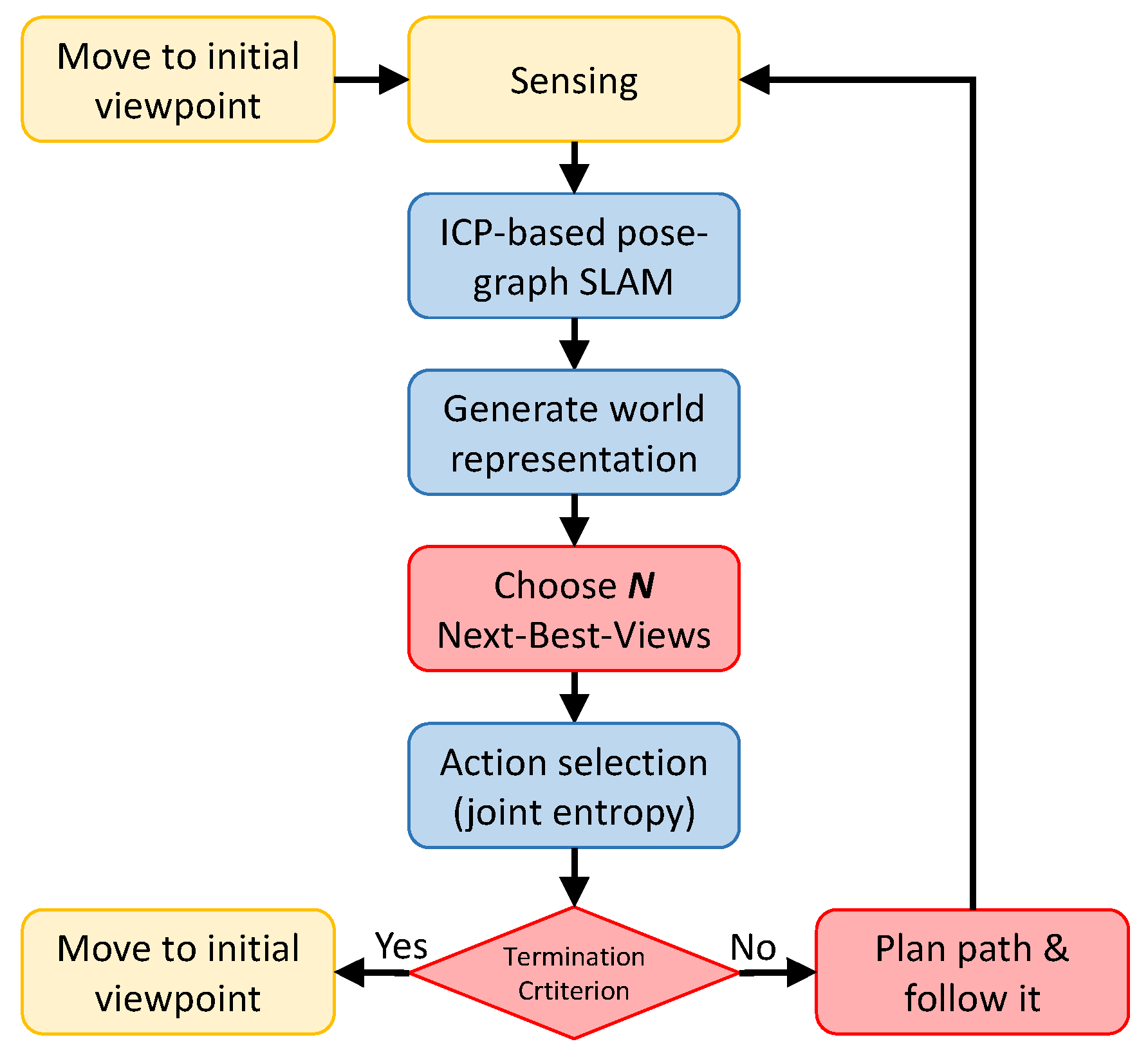
4] study the combined problem of SLAM with deciding where to move next in order to build the map as efficiently as possible. The proposed method consists of the following steps (see
Figure 1). The autonomous vehicle moves to a viewpoint and senses the environment using a mapping sensor; then, this data is used to correct both the robot position and the position of all previous viewpoints using a pose-graph algorithm. Next, the data gathered at each viewpoint is combined in a single octree that represents the world. A view planner calculates a set of candidate viewpoints to continue the exploration using this world representation. Thereafter, an action selection mechanism estimates the entropy reduction for each candidate, taking into account the map information provided by this viewpoint (i.e., the reduction of the entropy on the map), and the information provided by the viewpoint in order to close some loop with the viewpoints previously seen (i.e., the reduction of the entropy in the state of the vehicle). The candidate who optimally reduces the combined entropy on the map and the state of the vehicle is selected. If the termination criterion (i.e., coverage, number of scans, elapsed time, etc.) is not reached, a path planner computes an obstacle-free route to the selected viewpoint; the vehicle is commanded to follow it, and once reached, the process is repeated. Once any of the above mentioned termination criteria are reached, the exploration concludes and the vehicle returns to its initial position by planning an obstacle-free path.
In our proposal, the pose-graph SLAM method is responsible for precisely maintaining a good estimate of the vehicle trajectory and the location of each viewpoint while the mapping module recomputes the aggregated octree representation of the scene, merging the scans gathered at each viewpoint.
The proposed exploration method was devised for an AUV equipped with a multibeam sonar mounted on a pan and tilt device able to gather dense 3D point clouds, but it could be easily adapted to systems with other range sensors, such as laser scanners or stereo cameras. Although getting a scan moving a multibeam sonar with a pan and tilt system takes a few seconds, the quality of the point cloud obtained is much better if both are correctly synchronized, than the one that would be obtained with the usual technique in the state of the art, i.e., moving the robot with the sensor rigidly attached to it, since the uncertainty in the vehicle’s motion is greater than that in the positioner’s motion and the time to complete a scan is reduced to a fraction.
The pose-graph algorithm takes as input, the odometry measured by the robot as it navigates from one viewpoint to another and the 3D point cloud gathered at each viewpoint. The algorithm computes motion constraints between the two robot locations using the iterative closest point algorithm (ICP) [
5], a common approach for underwater robot navigation [
6,
7]. However, one of the main drawbacks of using ICP is the difficulty in assessing the quality of the computed motion constraint. In this paper we propose a novel, closed-form formulation based on the first order error propagation. When the function
to study is known explicitly, its Jacobian could be obtained by taking all the partial derivatives of
. However, in the ICP case there is a minimization that defines an implicit function between the data and the results [
8]. So, to calculate its Jacobian,
being a non explicit function, we propose to use the implicit function theorem.
The action selection mechanism chooses the viewpoint that most reduces the entropy. However, if after analyzing all the candidates proposed by the view planner, the smallest vehicle uncertainty exceeds a predefined threshold, the action selection mechanism may decide to return to an already visited viewpoint to keep its uncertainty under this threshold.
The interface with the view planner is the following. The input is a world representation, in the form of an octree, and the current robot position. The output is a set of candidate viewpoints that maximize the world exploration. For each viewpoint the view planner must provide its position and orientation and the number of unknown cells expected to be observed from it. Any view planner capable of providing this interface could be used within this framework.
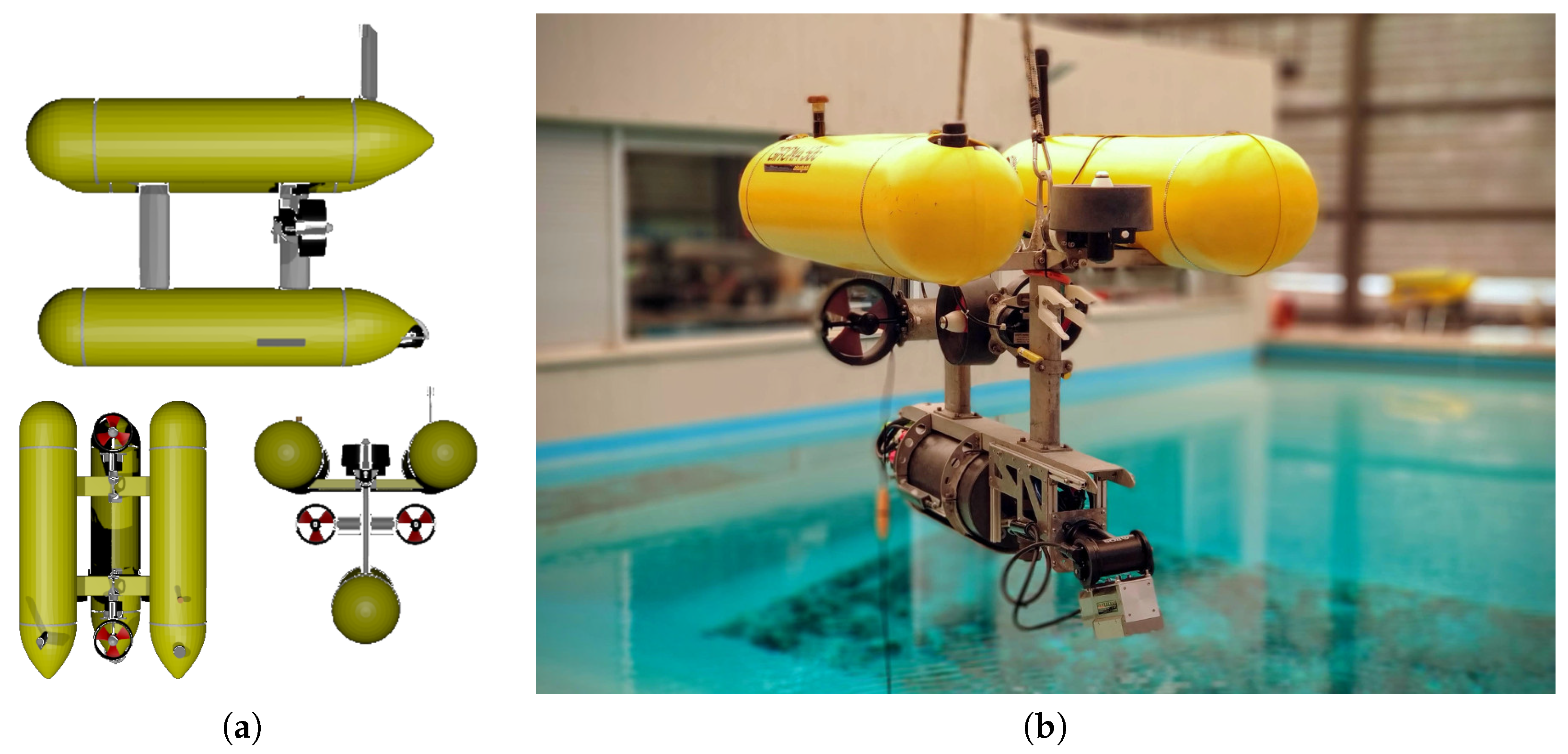
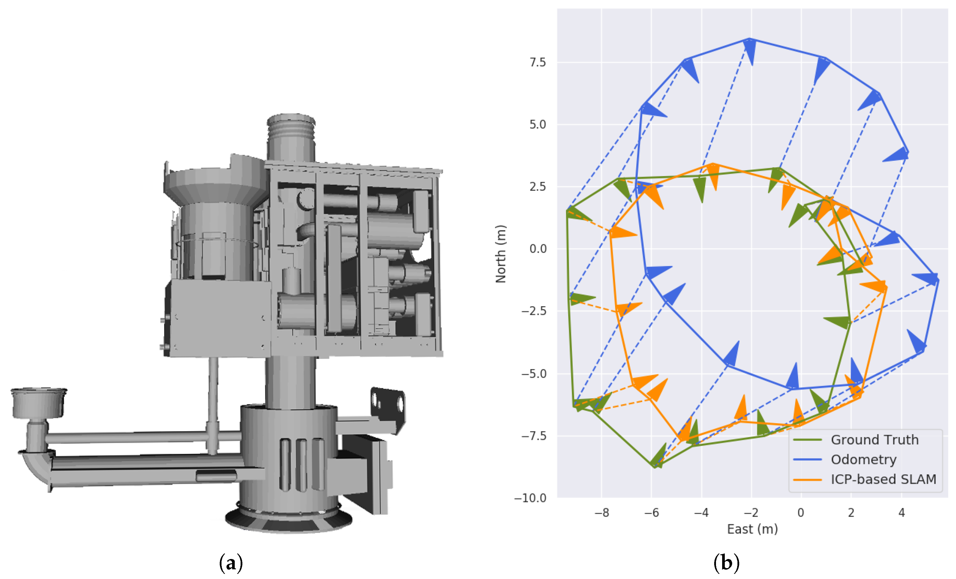
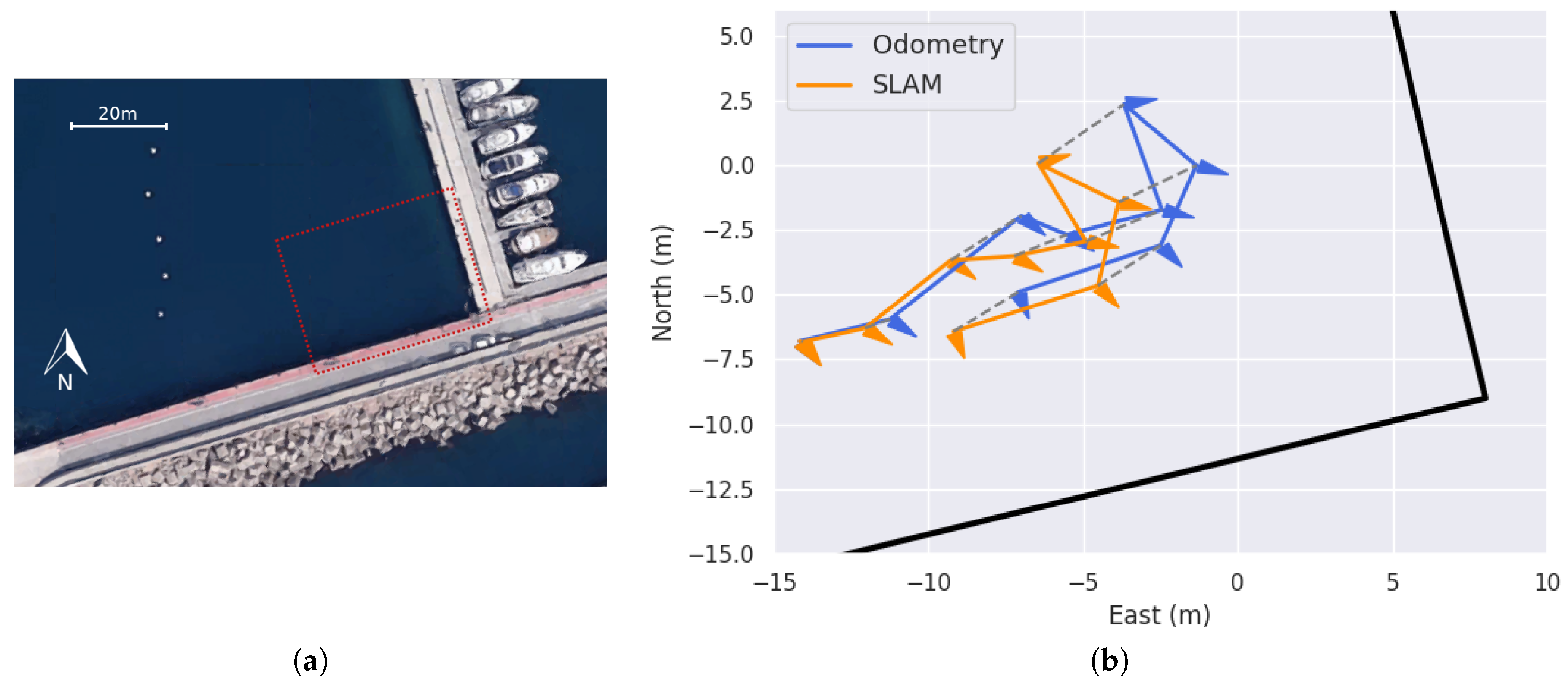
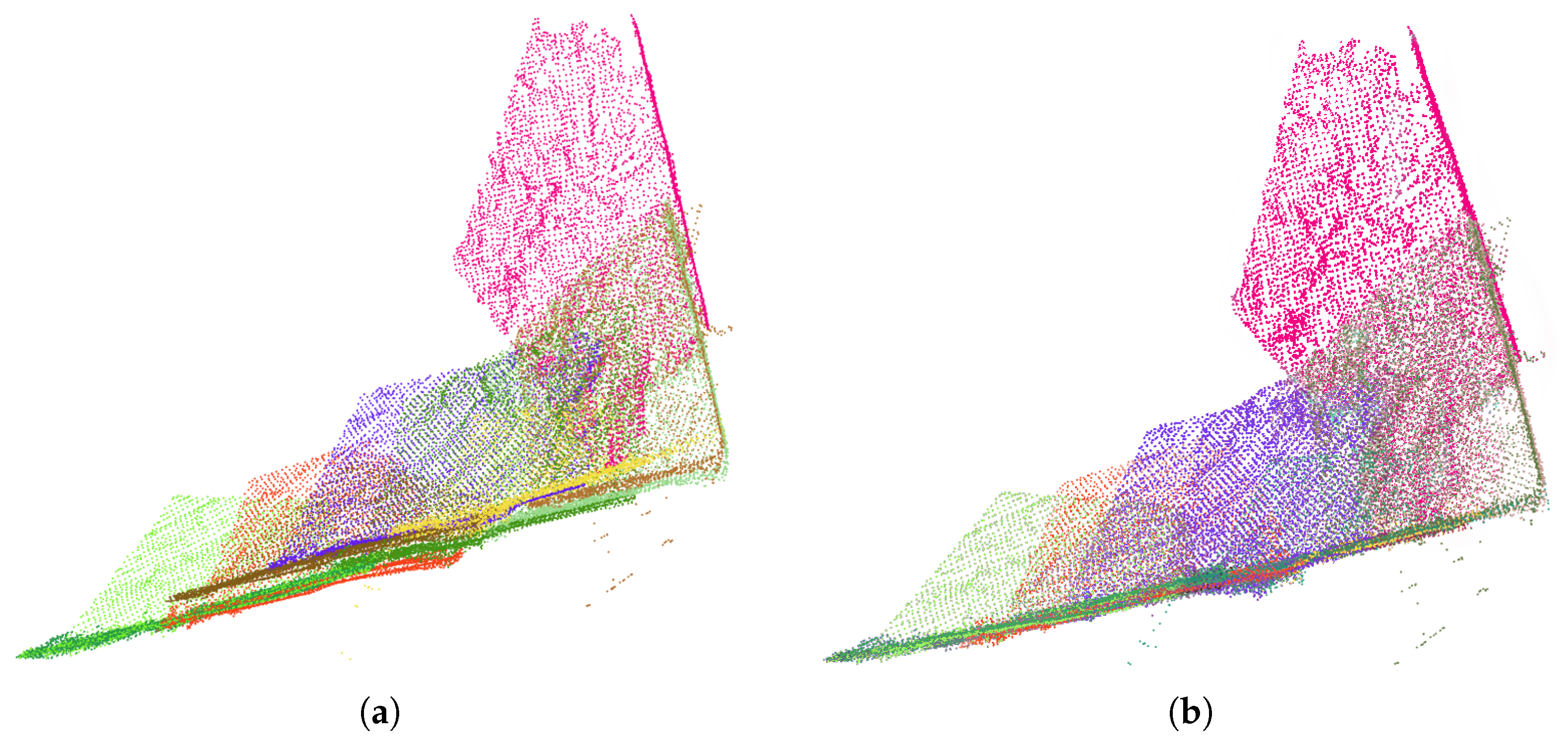
To evaluate the proposed exploration system several tests have been conducted using the Girona 500 AUV [
9], both in simulation and in real scenarios. Results demonstrate the benefits of using an active SLAM strategy. The accuracy of the pose-graph SLAM, that implements the new closed-form method to estimate the uncertainty in the ICP registers, has been analyzed and the action selection mechanism that allows to keep a low uncertainty in the vehicle state while maximizing the coverage.
The proposed framework endows AUVs with the necessary capabilities to undertake mapping and inspection missions in a priori, unknown, complex scenarios as it limits their drift, and consequently, allows to create more consistent models with a greater degree of coverage. In addition, the framework is generic enough to be adapted to other vehicles, sensors, domains or view planners than those discussed here.
The rest of the paper is structured as follows. First, several works related to view planning, localization and mapping, and exploration frameworks, specially those applied to underwater vehicles, are reviewed in
Section 2. Next,
Section 3 defines the pose-graph SLAM algorithm and the action selection mechanism that make up the proposed active SLAM. The closed-form solution to estimate the ICP error propagation is also presented in this section. Results for each algorithm and for the whole framework are reported in
Section 4 before conclusions.
2. Related Work
The objective of this work was to develop an exploration framework so that AUVs have the capacity to explore a priori, unknown, complex scenarios. To this end, we propose to combine SLAM and view planning techniques with an action selection mechanism to create an active SLAM framework for exploration tailored to AUVs. Relevant works related to SLAM, view planning, and exploration in different domains are presented below.
The first works about the autonomous exploration of an unknown environment date back to the 70s with the well known art gallery problem [
10]. However, it was not until the seminal work of Yamauchi [
11] that autonomous exploration got more attention from the robotics community. Yamauchi proposed a view planner, based on a frontier-based approach, that has been the starting point for many other works in the view planning field. Whaite and Ferrie [
12] presented the first uncertainty driven strategy for acquiring 3D-models of objects. However, they do not consider the uncertainty in the sensor pose. Despite some exploration solutions that claim to be robust against these uncertainties in the vehicle/sensor pose estimation [
13], when absolute positioning sensors are not available, it is necessary to localize the vehicle while mapping the environment to avoid corrupted maps.
The concept that an exploring robot has different actions to perform and it must choose the one that produces the maximum information was proposed by Feder et al. [
14]. Bourgault et al. [
15] also addressed the problem of maximizing the accuracy of the map building process during exploration by adaptively selecting control actions that maximize localization accuracy. The core of their framework consists of maximizing the information gain on the map while minimizing the uncertainty of both vehicle position and map features in the SLAM process. This concept has been exploited by many later publications, including ours. Sim and Roy [
16] showed the problem of using relative entropy as an object function. They point out that, although it is possible to quickly reduce the uncertainty of a distribution in some dimensions using this metric, in other dimensions there is no information gain.
Almost all the proposals presented during the late 90s and early 00s were based on the fact that the environment contains landmarks that can be uniquely determined during mapping. In contrast to this, Stachniss et al. [
17] presented a decision-theoretic framework that makes no assumptions about distinguishable landmarks. This framework simultaneously considers the uncertainty in the map and in the pose of the vehicle to evaluate potential actions using an efficient Rao–Blackwellized particle filter. In Vidal et al., [
18], the joint robot and map entropy reduction problem is faced using robot and map cross correlations obtained by an extended Kalman filter (EKF) that implements a visual SLAM. Valencia et al.’s work [
19] was similar to Stachniss et al.’s but used a pose-graph SLAM (i.e., a global approach able to optimize the whole trajectory) instead of a particle filter (i.e., a filter approach that optimizes only the current state). Additionally, their proposal takes into account the cost of long action sequences during the selection of candidates using the same information metrics to keep the robot localized during the path execution. Although these works have focused on mobile robots, exploring in most cases 2D scenes, there are also a good number of articles where exploration is performed by autonomous aerial vehicles in 3D environments [
20,
21]. However, like the exploration algorithms for 3D object reconstruction [
22,
23], the localization of these systems is normally solved and the methods focus mainly on the view planning and not on the active localization.
For the underwater domain, to the best of the authors knowledge, there are no works that combine localization, mapping, and exploration. In fact, most of the explorations carried out nowadays by AUVs are limited to follow a predefined mission that consists of flying over the sea bottom at a safe distance while acquiring data [
24]. It is possible to find works focused on view planning and others focused on SLAM but none that combine both techniques in a 3D scenario without a priori knowledge. Moreover, as several authors have stated [
17,
19], a straightforward combination of a view planner and a SLAM strategy is not sufficient to ensure a drift-free map with a high degree of coverage, which is why we propose an active SLAM solution. One of the few methods in which an AUV autonomously explores a complex structure was proposed by Englot [
25]. The method is focused on sensor coverage and uses a sampling-based strategy to guide the vehicle. However, a model of the object to map is required. We have also presented several works regarding underwater exploration. The first one was an iterative framework [
26], in which, starting from a low resolution a priori model, an exploration path is computed off-line an executed on-line in parallel with a SLAM algorithm that keeps the vehicle drift-bounded. The process is repeated until the desired resolution and coverage are reached. Despite the fact that the method combines an off-line view planning and SLAM, it does not check if the resulting trajectory will allow the SLAM algorithm to keep the localization uncertainty bounded, enforcing only some overlap between viewpoints. We have also presented solutions that do not require a preliminary map, but that do not localize the vehicle while exploring the 2D [
27] or 3D [
3] scene, nor use the robot state uncertainty to drive the exploration.
Underwater SLAM has attracted more attention from researchers than underwater exploration. Several works present solutions about how to map a complex underwater structures while localizing the vehicle with respect to it. A good example of this are the works of Vanmiddlesworth et al. [
6] and Teixeira et al. [
7] that use an ICP-based pose-graph SLAM algorithm. To decide if the ICP registers were valid, they used a fitness score that represents the normalized sum of squared distances between corresponding points in the register. Nevertheless, how the uncertainty of each register was estimated was not discussed by either. This problem affects all domains, not only the underwater one. Common solutions to estimate this uncertainty are based on Monte Carlo algorithms, that can not be used online due to their high computational cost [
28], or covariance estimation methods that rely on the Hessian objective function [
29].
3. Methodology
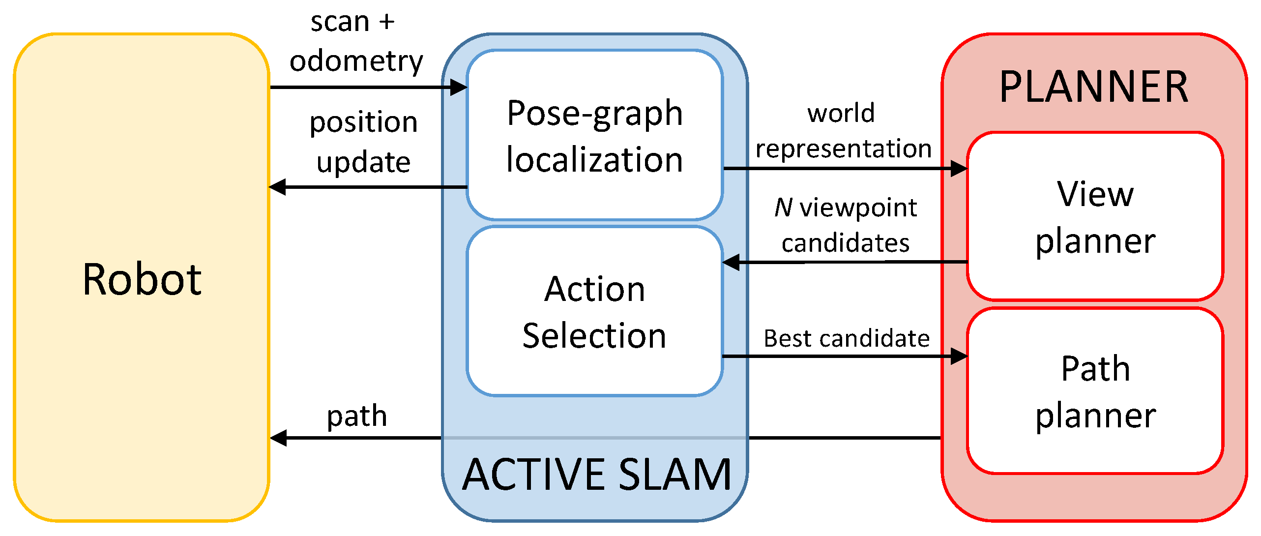
The proposed active SLAM strategy contains a pose-graph localization algorithm that uses scan matching to compute the registers between scans, and an action selection mechanism that makes use of the joint map and state entropy to choose the next-best-viewpoint to explore from a set of viewpoints proposed by a view planner. As shown in
Figure 2, the robot provides the scan (i.e., a point cloud) and the odometry between viewpoints to the pose-graph algorithm. A new position in the localization graph is created, and using the ICP algorithm, the current scan is registered with all previously gathered scans that may overlap with it (see
Section 3.1). The uncertainty for each register is estimated (see
Section 3.2), and finally, the pose-graph is optimized. With the optimized position for each viewpoint, a low-resolution world model (i.e., an octree) is built, merging all the scans. This representation is used by the view planner to calculate a set of candidate viewpoints and by the path planner to obtain a free path from the current position to the next-best-viewpoint.
This article focuses on the active SLAM part of the system, whereas the view planner used is the one reported in [
3]. Note, however, that this exploration framework could use any view planner capable of computing a set of candidate viewpoints that further explore the scene and the number of unknown cells observable from them, given an octree that represents the already explored region.
From the set of candidate viewpoints computed by the view planner, the action selection mechanism calculates the decrease in entropy that would be achieved by observing the scene from each of them. First, it computes the mutual information gain by closing a loop between each candidate and any previously visited viewpoint in which there is overlap. To compute this information gain, the uncertainty of the previously-visited viewpoints that can be obtained from the pose-graph algorithm, is used. The resulting state entropy reduction is combined with the map entropy reduction calculated using the number of unknown cells observable from the candidate viewpoint, as detailed in
Section 3.3. The viewpoint with the greatest state-map entropy reduction is then chosen. A rapidly-exploring random tree star (RRT*) path planner is used to drive the robot from its position to the desired viewpoint [
30].
The following subsections explain the details for the ICP-based pose-graph algorithm, the way in which the uncertainty of each ICP register is computed, and how the action selection mechanism computes the map and the state entropy reduction and combines them to select the next viewpoint to visit.
3.1. ICP-Based Pose-Graph Algorithm
When no absolute navigation sensors are available, the localization of the AUV is based on a dead reckoning filter that integrates measurements from on-board navigation sensors. These sensors are: a Doppler velocity log (DVL) that measures the AUV linear velocity, a pressure sensor that measures the vehicle’s depth, and an attitude and heading reference system (AHRS) that provides orientations and angular velocities. For the experimental part we used the AUV Girona 500 [
9], with 4 controllable DoFs—
x,
y,
z, and
(
), whilst being very stable in
and
. Of the 6 DoFs, the
z term can be directly measured from a high accuracy pressure sensor (i.e., < 0.01% of the range) and a tactical grade AHRS provides
and
measurements with accuracies over 0.1°. However, there is no on-board sensor able to provide drift-free measurements for
x,
y, and
once the AUV is submerged. A compass could be used to mitigate the drift in heading but this can induce further problems when working close to structures which are common in many inspection-like missions [
7].
The drift in
x,
y, and
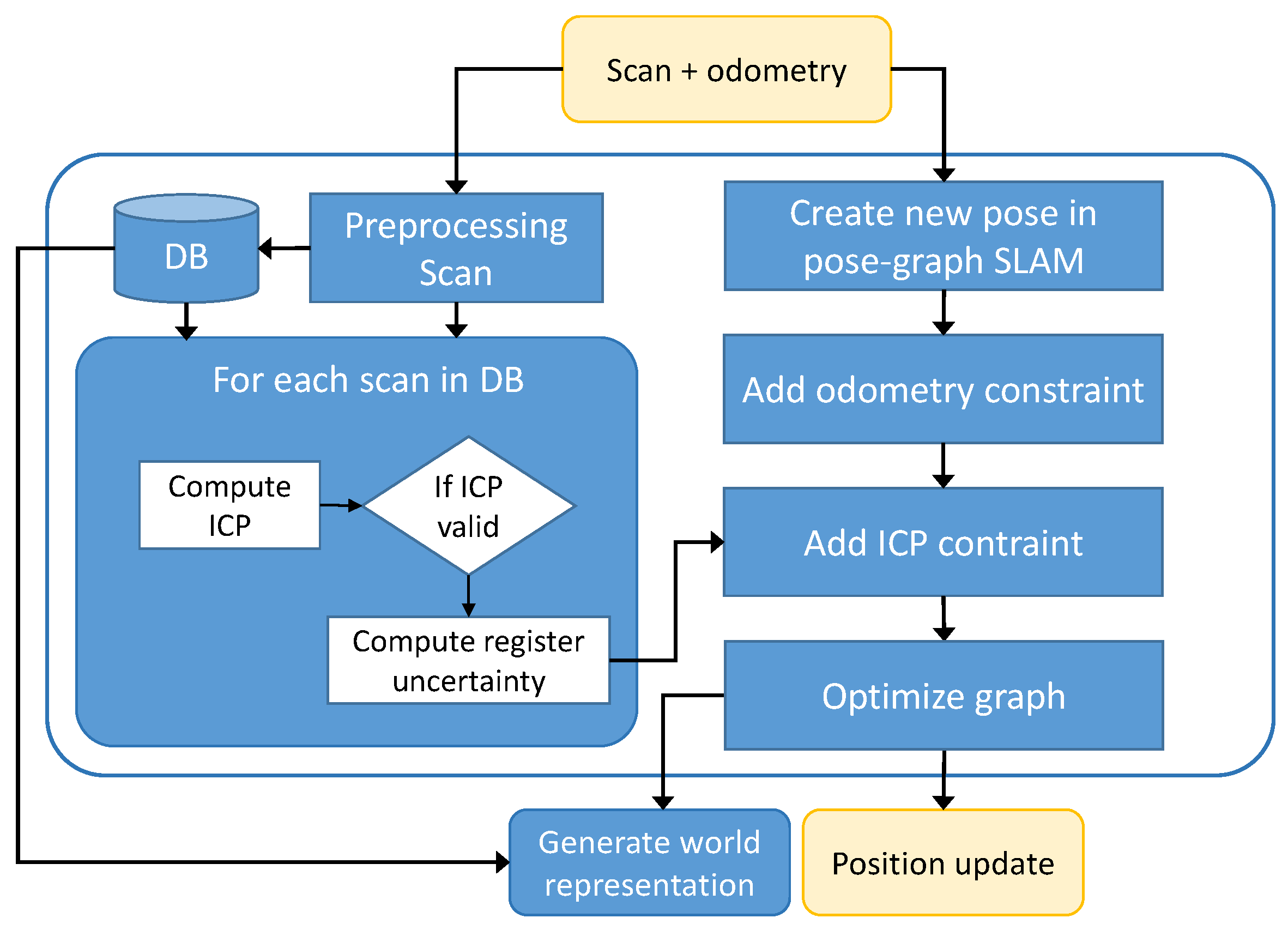
can corrupt the world model and cause the robot to end up colliding with some obstacles in the environment. To avoid that, an online, ICP-based pose-graph SLAM algorithm is implemented. This algorithm estimates the vehicle position and orientation at each viewpoint (i.e.,
). The difference between the position estimated by the dead reckoning filter and the pose-graph SLAM is used to correct the former. The procedure shown in
Figure 3 is executed every time that the vehicle reaches a viewpoint and gathers a new scan.
The ICP-based pose-graph algorithm uses as input, a scan, containing the gathered point cloud, the odometry from the previous viewpoint () according to the dead reckoning filter running in the AUV, and the values that are not going to be optimized ([z, , ]). The ICP registration pipeline filters the point cloud using a statistical outlier removal filter and downsamples it using a grid filter. Next, normals are computed. The resulting filtered point cloud with normals () is stored.
To check if the last scan gathered from viewpoint
may overlap with any previous scan gathered from viewpoint
, where
, the overlap of the mapping sensor FoV between these two viewpoints, is computed. If the overlap is over a threshold, each local point cloud
and
are transformed to the world frame (i.e.,
w and
w). Next, the ICP algorithm is applied and a rigid transformation (
i) is obtained. Because all the localization is carried out in SE2, the ICP algorithm is restricted to estimate
i also in SE2. The composition of the original transformation between the viewpoints and the result of the ICP register (i.e.,
i) is added in the pose-graph as a loop closure between
and
. The scan matching pipeline was implemented using the point cloud library (PCL) [
31].
In parallel with the scan registration, the pose-graph is created. The first viewpoint (
) is used to fix the initial pose in the graph. Subsequent viewpoints generate new poses in the pose-graph connecting each new viewpoint to the last one using the odometry provided by the dead reckoning filter. The following state augmentation equation is used:
All the constraints resulting from the scan matching pipeline are also added in the pose-graph connecting the current pose with all loop closing poses. Once all the constraints have been set, the graph is optimized and the position obtained for the last pose is sent back to the dead reckoning filter to correct the estimate of the AUV current position. The Ceres library [
32] was used to implement the graph optimization.
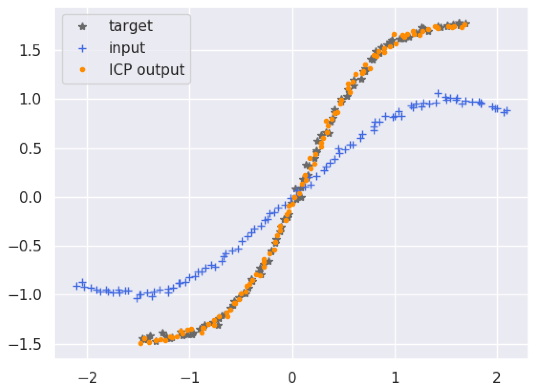
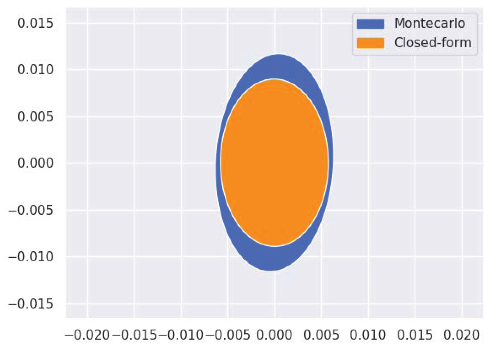
3.2. ICP Error Propagation Estimation
After matching two scans using the ICP algorithm, the rigid transformation that better aligns them is used to create a new constraint in the pose-graph together with an estimation of its uncertainty. ICP algorithms do not compute this uncertainty and only provide some metrics, such as the sum of squared distances from the source point cloud to the target, to assess how good the matching is. Since the ICP algorithm consists of minimizing an error function iteratively, it is not possible to express it with an explicit function, and therefore calculate its Jacobian to propagate the error in the data to obtain this uncertainty. For this reason, we propose using the implicit function theorem [
33] to estimate how the uncertainty in the matched point clouds is propagated.
Given a system
the implicit function theorem states that, under a mild condition on the partial derivatives (with respect to the
) at a point, the variables
are differentiable functions of the
in some neighborhood of the point. Because these functions can generally not be expressed in closed form, they have to be implicitly defined by (
2).
The implicit function theorem assumes that
is the continuous and partial derivative in a neighborhood
, such that
Then, there exists a neighborhood of
in which there is an implicit function
such that:
Given a reference set of points
, where each point is defined as
, and a second set of points
, where each point is defined as
, the ICP algorithm associates each
with the closest
. In other words, given two point clouds (
and
) related by
where
is a rotation matrix and
a translation vector
, the ICP algorithm estimates the transformation values (
,
,
) that minimize the cost function
where
Expressing the previous equation using vectors for
n points we obtain:
where
To minimize the cost function (
6), it has to be partially derived by
,
, and
and made equal to zero. See
Appendix A for its development.
The resulting
is an implicit function that represents the minimum cost of the ICP algorithm and fulfills the conditions for applying the implicit function theorem. To apply it, the partial derivatives (
) of
with respect to the known variables (i.e., the set of points
and
) and the partial derivatives (
) with respect the unknown variables (i.e.,
,
, and
) must be computed:
where
and
Therefore, the error in the point clouds
P and
Y (i.e.,
and
) can be propagated according to
. It is worth noting that to compute
, only the transformation
and the association
, both resulting from the ICP algorithm, are required.
3.3. Joint Map and State Entropy
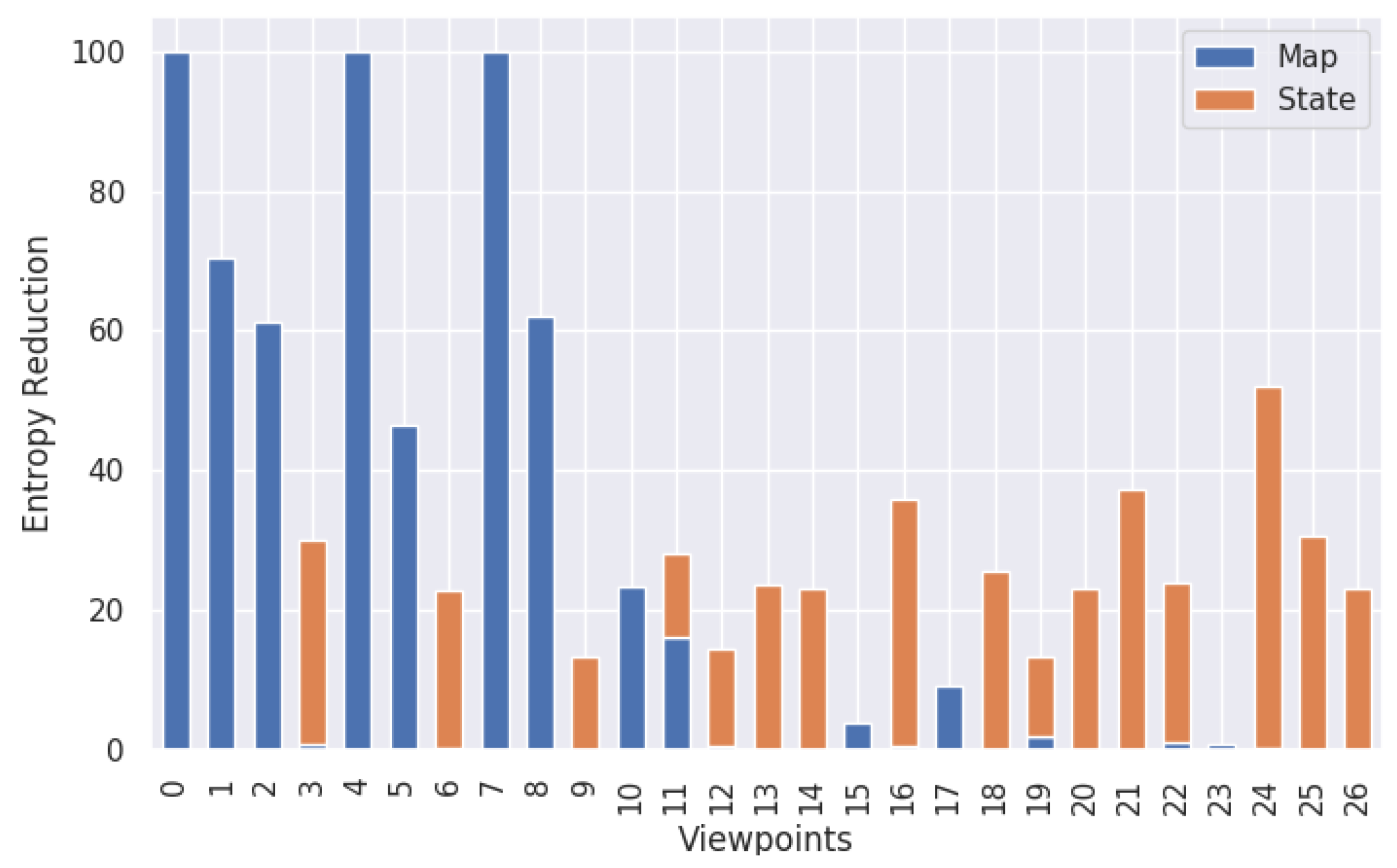
As discussed in the introduction, the simple combination of a SLAM algorithm and a view planner is not sufficient to ensure a consistent exploration. For this reason we included a third element that decides which viewpoint, of all those proposed by the view planner, should be visited next. This action-selection mechanism combines the information gained from the exploration of new regions with the vehicle state estimation improvement resulting from revisiting known locations. This measure is known as the map and state joint entropy.
If all motions and observations are given, the map and state joint entropy can be expressed as the state entropy plus an average of the entropy for all infinite maps resulting from all infinite states
x weighted by the probability of each state [
17]:
This equation can be approximated as:
where instead of computing the map entropy averaged for all infinite possible maps, we compute it only for the mean pose estimates
. The
factor is added to scale the map entropy depending on the probability distribution.
Because we are only interested on the entropy reduction, the following equation can be used instead:
Therefore, the action selection mechanism evaluate the reduction of joint entropy in these two terms for each of the candidate viewpoints and select the best one.
3.3.1. State Entropy
To compute the reduction in the state entropy, we assume
being
where
is the sensor registration covariance and
is the innovation covariance computed as
and
are the Jacobians of
h with respect to poses
i and
k evaluated at the state means
and
(see
Appendix B),
and
are the marginal covariances of
and
respectively, and
is their cross correlation [
34]. The
h function relates an observation
,
,
, and
being the distances between states
and
in world coordinates. They can be expressed as:
The value of
cannot be known in advance using (
9). Therefore, it is assumed that for the same sensor, configuration. and scene,
will be similar to previously computed ones and an average of them is used.
Because
depends on the number of loops that can be closed, the sensor FoV overlap described in
Section 3.1 is used to check how many loop closures exist between the analyzed viewpoint and any of the viewpoints already visited. Therefore, matrices in (
13) increase its dimensions according to the number of loops that can be closed.
3.3.2. Map Entropy
To measure
using an octree, according to the common independence assumption about the cells, the entropy of a map
m is the sum over the entropy values of all cells [
17]:
where
c is the cell probability and
l the length of the side of a cell.
If the view planner used provides the number of unknown cells in
m that are observable from each proposed viewpoint (i.e.,
), the map entropy reduction
can be approximated by:
The factor accounting for the path probability distribution
in (
10) has an intuitive meaning: explorations made from well-located viewpoints produce more accurate maps than those made from uncertain locations. In fact, if we add new scans to the map from viewpoints where the robot has large values of marginal covariance, this can increase the entropy of the map as it is possible to register point clouds that, although being similar to each other, are clearly very distant. The inverse of the determinant of the current state marginal covariance is used to weight the map entropy reduction:
The parameter can be used to fine tune the weight of the map with respect to the state.
5. Conclusions
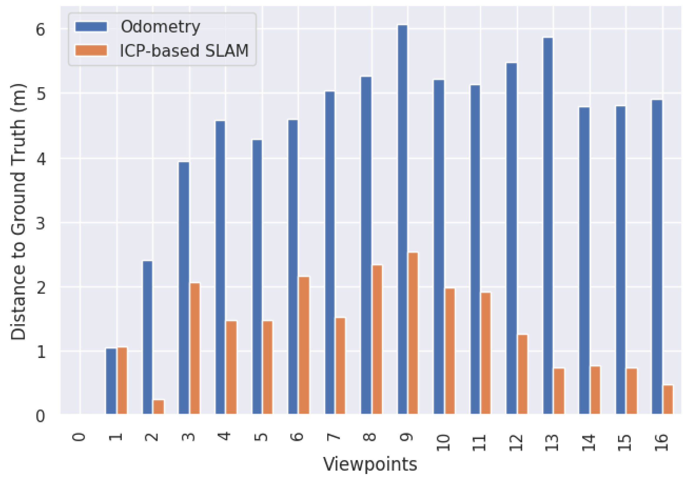
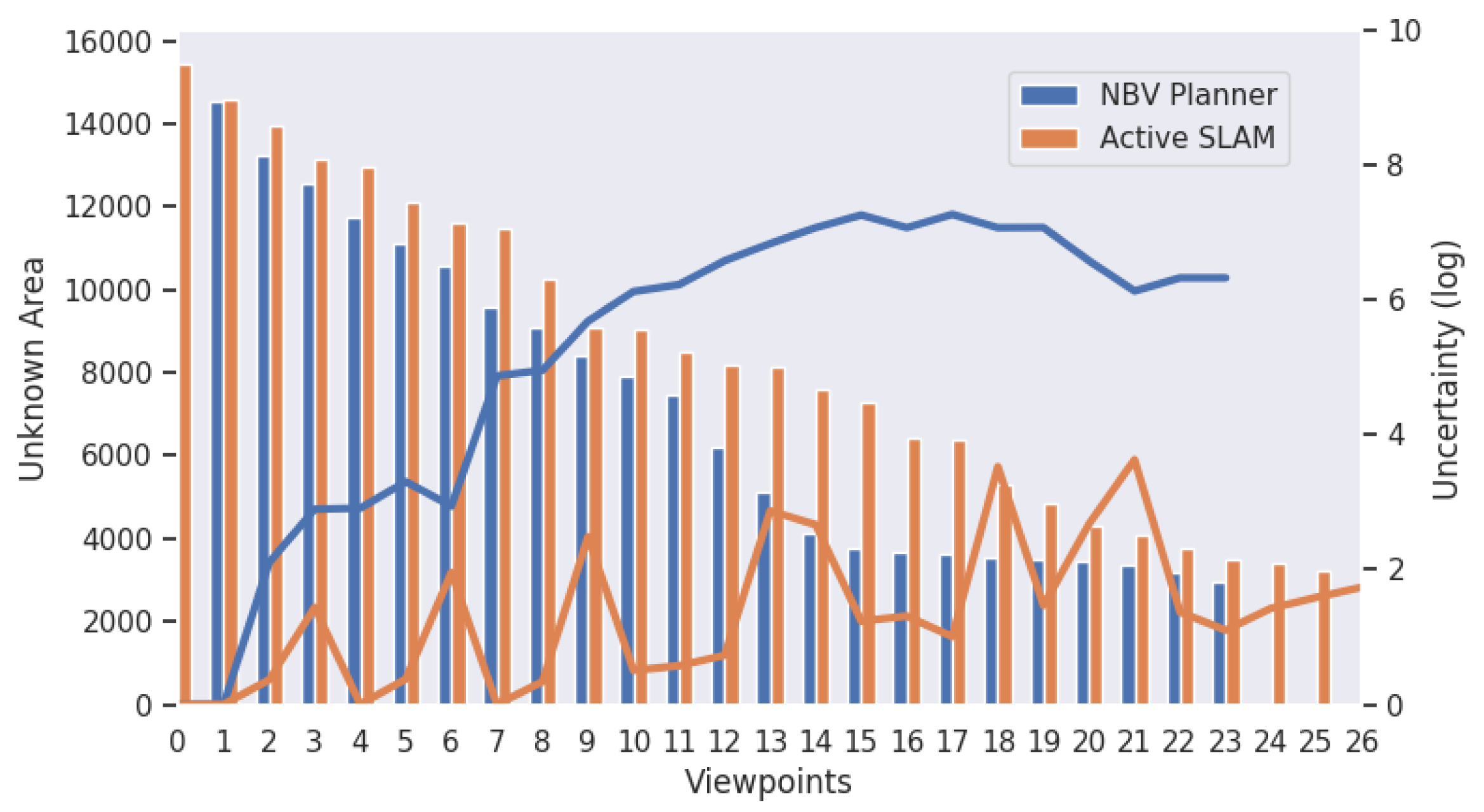
A new exploration framework based on an active SLAM strategy is proposed herein. The system was tailored to AUVs and was conceived to be used in complex environments, with a strong 3D component, where there is no a priori map. The methodology employed combines a view planner and a pose-graph based localization and mapping algorithm with an action selection mechanism. This mechanism decides the next viewpoint to visit taking into account which will be able to reduce the entropy in the map more and in the state of the vehicle jointly. The paper is focused on the localization and mapping algorithm and in the action-selection policy. The former was implemented using a standard pose-graph approach and using the ICP algorithm to register the point clouds gathered from different viewpoints. To compute the error propagation in the ICP algorithm, a closed-form solution was proposed. This solution allows one to compute a realistic covariance for each ICP register in real time. Compared to a Monte Carlo simulation, the method produces similar but slightly optimistic results. The proposed pose-graph SLAM pipeline was tested with data obtained through simulations and with data collected with the Girona 500 AUV in a harbor. As expected, in both situations, the trajectory and the world model obtained, once having applied the optimization, showed better correspondence with reality than the ones obtained only with the AUV odometry. The use of an action-selection mechanism led to the natural emergence of a new exploration behavior in the robot. The fact of weighing the exploration (i.e., examining unknown regions) and the improvement of the robot state (i.e., revisiting already known positions), using in both cases, the entropy reduction, causes the following behavior: whenever the uncertainty in the vehicle state is small, the active SLAM maximizes the exploration of new regions, while when this uncertainty is large, the vehicle tries to reduce it by revisiting known regions with small uncertainty. When possible, the action-selection mechanism chooses viewpoints in which both of the above goals apply.
The proposed framework is generic enough as it can be used in other domains or easily adapted to other scanning sensors, Moreover, it can make use of any view planner that takes as input, the robot location and an octree with the current exploration state and from this is able to generate a set of valid viewpoint candidates to further explore the environment.
As a future work, the two main limitations that have been identified when testing the active SLAM framework with different scenarios should be addressed. On the one hand, if the scene does not have enough features, the ICP algorithm is not capable of registering the point clouds, or, in the worst case, registers them poorly (e.g., when registering two flat surfaces). To solve this problem we propose extracting the 3D features of the point clouds first, to make a first coarse alignment, and only if this succeeds, completing the registration with the ICP algorithm [
36]. A second problem has been observed when the vehicle has to travel long distances close to obstacles in order to move from one viewpoint to another. Since the vehicle position is only corrected in the viewpoints, this can cause the robot to collide with an obstacle. To avoid this, we propose developing a motion planning algorithm that ensures that the vehicle state uncertainty never exceeds a certain threshold during the entire route. Therefore, the vehicle should plan a path in which it is possible to close enough loops with previously visited regions to keep this threshold.

