Abstract
The rapid growing number of earth observation missions and commercial low-earth-orbit (LEO) constellation plans have provided a strong motivation to get accurate LEO satellite position and velocity information in real time. This paper is devoted to improve the real-time kinematic LEO orbits through fixing the zero-differenced (ZD) ambiguities of onboard Global Navigation Satellite System (GNSS) phase observations. In the proposed method, the real-time uncalibrated phase delays (UPDs) are estimated epoch-by-epoch via a global-distributed network to support the ZD ambiguity resolution (AR) for LEO satellites. By separating the UPDs, the ambiguities of onboard ZD GPS phase measurements recover their integer nature. Then, wide-lane (WL) and narrow-lane (NL) AR are performed epoch-by-epoch and the real-time ambiguity–fixed orbits are thus obtained. To validate the proposed method, a real-time kinematic precise orbit determination (POD), for both Sentinel-3A and Swarm-A satellites, was carried out with ambiguity–fixed and ambiguity–float solutions, respectively. The ambiguity fixing results indicate that, for both Sentinel-3A and Swarm-A, over 90% ZD ambiguities could be properly fixed with the time to first fix (TTFF) around 25–30 min. For the assessment of LEO orbits, the differences with post-processed reduced dynamic orbits and satellite laser ranging (SLR) residuals are investigated. Compared with the ambiguity–float solution, the 3D orbit difference root mean square (RMS) values reduce from 7.15 to 5.23 cm for Sentinel-3A, and from 5.29 to 4.01 cm for Swarm-A with the help of ZD AR. The SLR residuals also show notable improvements for an ambiguity–fixed solution; the standard deviation values of Sentinel-3A and Swarm-A are 4.01 and 2.78 cm, with improvements of over 20% compared with the ambiguity–float solution. In addition, the phase residuals of ambiguity–fixed solution are 0.5–1.0 mm larger than those of the ambiguity–float solution; the possible reason is that the ambiguity fixing separate integer ambiguities from unmodeled errors used to be absorbed in float ambiguities.
1. Introduction
Over the past two decades, the increasing number of satellites in Low Earth Orbits (LEOs) has found ever growing interest in space-based earth observations such as gravimetry [1,2,3], altimetry [4,5], radio occultation [6], and so forth. Among the key issues of these space applications is the precise knowledge of LEO satellites’ positions and velocities. With the help of spaceborne Global Navigation Satellite System (GNSS) receivers, LEO orbits can achieve an accuracy of 2–5 cm using precise GNSS orbit and clock products in post processing [5,7]. To support the timely delivery of onboard science products, the precise real-time LEO orbit is a necessity. Nevertheless, the latency and accuracy of real-time GNSS orbits and clocks have been a major hamper for accurate real-time LEO orbits. Currently, the accuracy of onboard real-time LEO orbits using Global Positioning System (GPS) broadcast ephemeris is around 0.3–0.5 m [8], which is sufficient for the attitude and orbit control system but far from the sub-decimeter requirement for many scientific missions [9]. In recent years, with the refinement of precise orbit determination (POD) models and strategies, real-time GNSS orbit and clock products with higher precision are provided by International GNSS Service (IGS) Real-Time Service (RTS) [10]. Using the state-of-the-art near-real-time orbit and clock products, Montenbruck et al. [11] demonstrated that the real-time reduced dynamic orbit of MetOp-A satellite could achieve an accuracy of around 5 cm.
Except for reduced dynamic orbit, the kinematic orbit is also an essential element for the real-time LEO satellite position. Different from the reduced dynamic POD, kinematic POD is a purely geometrical approach without using any information about LEO satellite dynamics, thus it is completely independent from the force models used for LEO POD [12]. As a result, the kinematic POD represents the following features: (1) the observation model of kinematic POD is much simpler than that of reduced dynamic POD, which leads to a smaller compute burden for onboard processing; (2) the positions determined in different epochs are relatively independent, so that they won’t be affected by the aberrant dynamic parameters that estimated previously, e.g., after an orbit maneuver; (3) kinematic POD is more appropriate for independent gravity field recovery since the dynamic parameters in reduced dynamic POD will absorb some gravitational orbit perturbations [3,13]. In addition, a commercial trend towards building global-coverage LEO constellations, for communication and navigation, has brought thousands of low-cost LEO satellites to the launch schedule [14,15]. Thus, the refinement of current POD strategies is needed to adapt the new situations. In addition, the continuous development of spaceborne GNSS receivers, e.g., multi-GNSS and multi-frequency tracking capability [16,17], is expected to further improve the kinematic POD accuracy via more observation resources and better observation quality. Thus, the kinematic POD will become more competitive in the near future. Theoretically, the kinematic POD can reach the same accuracy level as the reduced dynamic approach. However, the practical kinematic orbit usually presents inferior performance compared with the counterpart [18]. The main limitation of kinematic orbit accuracy is the short-term systematic errors caused by GNSS observation noises, poor geometric distributions, and satellite clock errors [19]. One of the effective approaches to alleviate these factors is to strengthen the observation model, e.g., by fixing the phase ambiguities to integer numbers.
Ambiguity resolution (AR) is a well-proven technique to significantly improve the accuracy of precise GNSS processing [20,21]. Due to the existence of uncalibrated phase delays (UPD) in both transmitters and receivers, which closely couple with phase ambiguities, the phase ambiguities usually lose their integer properties in GNSS parameter estimating. The whole estimation is thus weakened since the phase ambiguities are estimated as float values. Generally, there are two approaches to recover the integer nature of phase ambiguities: by forming double-differenced (DD) and by using zero-differenced (ZD) phase observations. The former eliminates most common UPDs between different signal paths of receivers and satellites, while the latter estimates and calibrates the UPDs on ZD phase observations of a single receiver. Several ZD AR methods have been proposed and developed for precise point positioning (PPP). Two representative ones are the UPD-based method [22,23] and the integer recovered clock (IRC) method [24,25]. The Centre National d’ Etudes Spatiales (CNES) and Collecte Localisation Satellites (CLS) have begun to provide GPS IRC products since 2009 [26] and Galileo IRC products followed in 2018 [27]. Geng et al. [28] and Shi et al. [29] compared the existing methods and verified that they were not only theoretical equivalent, but also showed similar position performance. Montenbruck et al. [19,30] performed post-processing POD for Sentinel-3 and Swarm satellites with CNES/CLS IRC products and reported about 30–50% orbit accuracy improvements compared with the float solution. Allende-Alba et al. [31] demonstrated that ZD AR could also improve the baseline precision in LEO satellite relative positioning.
In this contribution, we focus on improving the performance of real-time LEO kinematic POD through the ZD AR method. The onboard GPS observations from Swarm and Sentinel-3 satellites are processed for the validation of the proposed method. This article is organized in the following sections. Firstly, the detailed algorithms of epoch-wise ZD AR are discussed in Section 2. Then, Section 3 gives an overview of the processing strategies and data sets. Afterwards, the ambiguity fixing performance and its impact on POD are analyzed in Section 4. Finally, we come to a conclusion in Section 5.
2. Epoch-Wise Zero-Differenced Ambiguity Resolution
2.1. Observation Mode
The LEO onboard GNSS carrier phase and pseudo range observations at a specific epoch can be modeled as follows [32,33]:
where s, r, and j denote the GNSS satellite, LEO receiver and frequency, respectively; refers to the geometric distance from the satellite (at signal transmitting time) to the receiver (at signal receiving time) in meters; c is the speed of light in vacuum; and denote the satellite and receiver clock offsets in seconds; is the wavelength of frequency j in meters; and refer to the receiver-dependent and satellite-dependent phase biases in cycles while and denote the corresponding code hardware delays; is the integer phase ambiguity in cycles; refers the ionospheric delays at frequency j in meters, which leads a code delay and phase advance with similar magnitude; and are the sum of measurement noise and multi-path errors. The phase windup, phase center offsets (PCOs) and variations (PCVs) can be corrected according to the existing models [34].
The ionosphere-free (IF) combination carrier phase and pseudo range observations are regularly used to eliminate the first order ionospheric delay in the GNSS data processing. Here, the high-order ionospheric (HOI) terms are neglected since it was reported that they were not the main cause of LEO satellite systematic errors near the magnetic equatorial area. In addition, the orbit accuracy improvement with HOI terms corrected could be very limited [35,36,37]. The IF observation equations are formulated as follows:
where refers to the wavelength of IF combination phase observation (about 6 mm); is the IF combination phase ambiguity; and denote the IF receiver-dependent and satellite-dependent phase biases; and are the IF code hardware delays of receiver and satellite, respectively; and are the sum of IF measurement noise and multi-path errors.
In a typical PPP processing, the satellite clock offset is corrected with precise clock products. Since the clock products are commonly estimated by IF combination observations, they have assimilated the IF satellite code hardware delay and become . As a result, the satellite-dependent code hardware delay in Equation () will be eliminated when the observation combination employed in PPP (e.g., L1&L2 for GPS) is identical with that in precise clock product generating. In addition, the receiver clock offsets are inseparable with the receiver-dependent code hardware delay, so the estimated receiver clock offset will absorb the code hardware delay of the receiver, which can be expressed as . As a consequence, the phase ambiguity in Equation (3) absorbs both phase biases and the code hardware delays. The re-parameterized phase ambiguity thus loses its integer property and can be expressed as the sum of the integer ambiguity and its UPDs:
with
2.2. Zero-Differenced Ambiguity Resolution
In the ZD AR processing, the IF combination ambiguity is usually formulated as the combination of wide-lane (WL) and narrow-lane (NL) ambiguities:
where refers to NL wavelength, so is also called NL ambiguity in this equation. The ZD ambiguity resolution is technically conducted with a first WL and then NL process. The IF combination ambiguity is fixed as soon as both the integer WL and NL ambiguities are resolved.
Usually, WL ambiguities are derived from Melbourne–Wübbena (MW) combination [38,39], which is a geometry- and ionospheric-free linear combination formed with dual-frequency phase and code observations:
Inserting Equations (1) and (2) into Equation (9), the geometric distance , clock offsets ( and ), and ionospheric delay will be eliminated. Hence, the MW combination can be expressed as the linear combination of WL ambiguity and WL biases ( and ):
with
where and are the receiver-specific and satellite-specific WL biases in WL wavelength. The obtained WL ambiguity is not an integer number due to the existence of and . Fortunately, the fractional parts of these biases can be estimated through a least square adjustment using float ambiguities from a reference network [23,26]. Then, the fractional WL bias (WL UPD) of each satellite will be broadcast to PPP users for ZD AR.
At the user-end, by using the WL UPD products, the satellite WL UPD () can be removed. After the separation of , the receiver WL UPD () can be estimated via averaging the fractional parts of all the available WL ambiguities [40]. Afterwards, the integer value of WL ambiguity can be resolved by a round strategy:
With the WL ambiguity fixed, the corresponding float NL ambiguity can be calculated by integer WL ambiguity and IF combination ambiguity according to Equation (8):
Similar to WL UPDs, the satellite NL UPD products can also be obtained through a network solution. At the user-end, the satellite NL UPD is firstly separated from the float NL ambiguity () using the corresponding UPD products. Note that, if the IRC products are employed, the float NL ambiguity () will not contain the satellite NL UPD since it has been assimilated into a satellite clock offset (). Afterwards, the receiver NL UPD can be determined by selecting a reference NL ambiguity with highest elevation and fixing it to the nearest integer:
where refers to the receiver NL UPD; and denote the reference float NL ambiguity and corresponding satellite NL UPD, respectively. Then, the receiver NL UPD can be corrected for other NL ambiguities. However, due to the low precision of float NL ambiguities, the reference NL ambiguity may be biased by cycles and lead to a common shift for all other NL ambiguities. This integer common bias will be assimilated into receiver clock offset and doesn’t harm the ambiguity resolution.
After separating both the satellite and receiver NL UPDs, the NL ambiguity is close to the integer but still affected by unmodeled biases and random errors. Different to WL ambiguity, the NL ambiguity’s wavelength is around 11 cm and is more sensitive to these errors. Thus, the LAMBDA [41] method rather than the round strategy is employed to search for the optimal integer solution of the NL ambiguity. Once both the WL and NL ambiguities are fixed to integers, the IF combination ambiguity can be calculated according to Equation (8). Then, the integer constraints will be exploited to the observation equations, so as to get a better POD estimation.
3. Real-Time Kinematic POD Strategies and Data Sets
3.1. POD Strategies
Based on the ZD AR algorithms in Section 2, the improved real-time kinematic LEO POD strategy is discussed in this subsection. Compared with the post-processing LEO POD, the use of ZD AR in a real-time situation needs to overcome the following additional difficulties:
- The relatively worse accuracy of GNSS orbit and clock, which directly restricts the LEO real-time POD accuracy. The inferior position accuracy thus leads to the less accurate and less reliable float ambiguities.
- The relatively worse quality of UPD product, which directly affects the properly fixing of ambiguity.
- Epoch-by-epoch filtering vs. Batch processing. In post processing, the ZD AR is performed for each pass, i.e., GNSS signal tracking arc. The float ambiguities are estimated with the whole observations of the tracking arc with high accuracy and reliability. Thus, the ZD ambiguities could be easily fixed via a round strategy [30]. When it comes to the epoch-by-epoch filtering, the ZD AR is performed for every individual epoch using epoch-estimated float ambiguities. As a result, the ambiguity fixing strategy must be determined very carefully.
In consideration of these factors, the proposed strategy is illustrated in Figure 1, including the following steps:
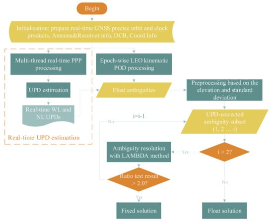
Figure 1.
The flow chart for LEO real-time kinematic POD using ZD AR.
Firstly, we need to prepare the necessary data for LEO POD e.g., real-time GNSS precise orbit and clock products, antenna and receiver information, Differential Code Biases (DCBs), etc. Then, the real-time PPP is performed on each station of a global-distribution reference network, with their coordinates fixed to IGS weekly-resolved solution. Here, to accelerate the data preparing and processing, the multi-thread technology is exploited for data downloading, merging, preprocessing, and parameter estimations [42]. With the float MW and IF combination ambiguities resolved, the real-time WL and NL UPD estimation can be processed epoch by epoch as described in [23]. In addition, the real-time phase bias products can also be obtained from the IRC products provided by CNES/CLS. The preliminary results show a favorable consistency between our UPD results and the CNES/CLS solution.
At the LEO-satellite-end, the float solution for real-time kinematic LEO POD is performed continuously, with the receiver coordinates, IF combination ambiguity, and receiver clocks estimated epoch by epoch. Before the ambiguity fixing, a preprocessing based on the elevation and standard deviation is taken for float ambiguities. By using the real-time UPD products and the clean float ambiguity estimates, the real-time ZD AR is then performed with the first WL and then NL ambiguity fixing strategy. The WL ambiguities are resolved by a rounding strategy while a search strategy based on the LAMBDA method is applied to obtain the optimal integer values of NL ambiguities. However, when the float ambiguity solution is not accurate enough, e.g., under some poor observation conditions, it is tough to obtain reliable values for all ambiguities and the success rate will be too low. In consideration of such situations, the partial ambiguity fixing technology is performed to find a reliable ambiguities subset with high fixed priority, such as ambiguities at high elevation angle or with high accuracy of float solutions [41,43].
After the integer ambiguity resolution, the fixed failure-rate ratio tests are employed for the acceptance. Generally, the threshold value is empirically derived or chosen experimentally. In this study, a empirical threshold value of 2 is adopted, which was recommended and tested in [40,44,45]. If the integer ambiguity resolution is accepted, the corresponding integer constraints will be exploited to the observation equation and get the estimation with fix solution; otherwise, the float solution estimates will be output.
The processing strategies for the LEO real-time kinematic POD are listed in Table 1. The basic observations are the onboard undifferenced GPS L1+L2 IF combination code and phase observations with the sampling rate of 10 s. The phase center offsets (PCO) and phase center variations (PCV) for GPS antennas are corrected with igs_14.atx, which can be found at ftp://cddis.gsfc.nasa.gov. For LEO satellite antennas, the nominal PCO corrections are employed for Sentinel-3 and Swarm satellites. In addition, the PCV values of Swarm satellite antennas are previously estimated using the method mentioned in [46] while those of Sentinel-3 are currently absent. For real-time parameter estimation, parameters including receiver coordinates, receiver clock offsets, and phase ambiguities are estimated epoch by epoch using recursive least squares.

Table 1.
The processing strategy for LEO real-time kinematic POD.
3.2. Data Sets
For estimation of real-time UPD, a global tracking network consists of around 140 high-performance IGS and MGEX (IGS Multi-GNSS Experiment) stations is employed. Their geographical distributions are depicted in Figure 2.
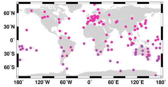
Figure 2.
The distributions of IGS and MGEX stations employed in real-time GPS UPD estimation.
Then, real-time kinematic POD is performed using Sentinel-3A and Swarm-A data from 1 August 2018 to 1 September 2018. Swarm is the first constellation mission of the European Space Agency (ESA) [48] and is dedicated to the exploration of the earth’s magnetic field, atmosphere, and gravity field [3]. Swarm mission consists of three identical Swarm satellites (A, B and C), which were launched into circular near-polar orbits on 23 November 2013. Swarm-A and Swarm-C were flying side by side with an initial altitude of 462 km, whereas Swarm-B was on a higher altitude of 511 km. However, the orbit altitudes of Swarm-A/C have been dropped to 444 km and that of Swarm-B is 502 km up to February 2017. The orbital inclinations are for Swarm-A/C and for Swarm-B. The local time of ascending node (LTAN) for the three satellites is drifting, which results in a 24 h of local time coverage every 7–10 months (The detailed information can be found in https://directory.eoportal.org/web/eoportal/satellite-missions/s/swarm#orbits). All the three Swarm satellites are equipped with identical POD instruments including GNSS receiver, Laser Retro-Reflector (LRR), and accelerometer.
Sentinel-3 is a multi-instrument mission to measure sea–surface topography, sea– and land–surface temperature, ocean color, and land color with high accuracy and reliability [49]. Sentinel-3A was launched on 16 February 2016, followed Sentinel-3B on 25 April 2018. Both the two satellites are on repeating frozen Sun-synchronous orbits ( inclinations) with the mean altitudes of 814.5 km, and the repeat cycle of 27 days. Sentinel-3B satellite is on an identical orbit to Sentinel-3A but flown out of phase with Sentinel-3A. Considering the requirements of ocean color and sea surface temperature missions, the local time of descending node (LTDN) is designed to 10:00 a.m. (The detailed information can be found in https://sentinel.esa.int/documents/247904/351187/S3_SP-1322_3.pdf). In addition, Sentinel-3 satellites have the 7-year designed lifetime and their fuel are enough to support up to 12 years of continuous operations. The orbit determination for individual Sentinel-3 satellite is supported by a GNSS receiver, a Doppler Orbit determination and Radio-positioning Integrated on Satellite (DORIS) instrument, and an LRR for Satellite Laser Ranging (SLR). The detailed information about Swarm and Sentinel-3 missions is listed in Table 2.
Table 2.
Overview of Swarm and Sentinel-3 satellites.
However, the integer ambiguity resolution with onboard Swarm and Sentinel-3 GPS observations has been prominently hindered by the half-cycle carrier phase biases existing in their GPS receivers. Fortunately, this limitation could be overcome through a refined strategy for carrier phase generation out of raw measurements [30]. The corresponding modified GPS observations are now available on the ftp site: ftp://swarm-diss.eo.esa.int and website: https://scihub.copernicus.eu/gnss. The following research are based on the modified half-cycle-bias-free phase observations.
The Swarm mission provides both reduced-dynamic and kinematic 24-h POD products as part of Level2 products [35]. The POD strategy is daily updated with a latency of 21 days. As for Sentinel-3 satellites, three categories of POD products with distinct timeliness are generated by the Copernicus POD Service (https://sentinels.copernicus.eu/web/sentinel/missions/sentinel-3/ground-segment/pod/products-requirements):
- Near Real-Time (NRT) products are delivered with a latency of 30 min and a precision of 10 cm radial RMS;
- Short Time Critical (STC) products are generated with a timeliness of 1.5 days and a precision of 4 cm radial RMS;
- Non Time Critical (NTC) products are computed after several weeks in order to make use of high precision GPS orbits and clocks, thus the NTC products could achieve the highest precision of 3 cm radial RMS.
Unfortunately, the POD data sets of Sentinel-3 are only provided for August 2018 as preliminary test data. The full data and products of entire mission are not available now and expected to be published by the ESA in the near future. As a consequence, data in August 2018 are selected in our experiments for the better assessment of orbit accuracy.
4. Results
For the validation of the proposed method, we performed the kinematic POD for Sentinel-3A and Swarm-A satellites using ZD ambiguities resolution epoch by epoch to simulate the real-time situation. We also calculated the ambiguity–float solution for comparison. In this section, we begin with the analysis of ambiguity fixing rate and the Time to First Fix (TTFF). Afterwards, we assess the POD accuracy in terms of difference with post-processed reduced dynamic orbit products and SLR residuals. The phase residuals are also analyzed to further illustrate the impact of ZD AR on kinematic POD.
4.1. Ambiguity Fixing Results
In this subsection, the ambiguity fixing performance is evaluated in terms of the following aspects: ambiguity residuals, fixing rate, and TTFF. The ambiguity residuals are defined as the difference between the UPD-corrected ambiguity and its nearest integer. After subtracting the satellite and receiver UPDs, the float WL and NL ambiguities should be close to integer numbers. Therefore, the residuals distribution is a common quality index for the estimated UPD. For the purpose of illustration, the distribution of WL (left) and NL (right) residuals for day-of-year (DOY) 213 of 2018 is displayed in Figure 3. Both the two histograms are symmetric, bell-shaped and concentrate to around zero. It can be found that over 90% WL and 93% NL ambiguity residuals are within 0.15 cycles, which further confirms the high reliability of WL and NL UPD correction.
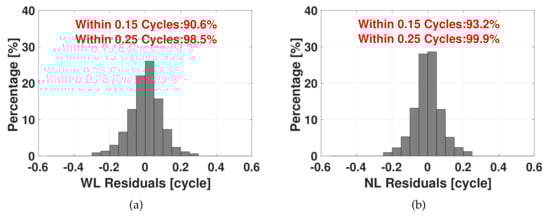
Figure 3.
Distributions of the estimated GPS ambiguity fractional parts after removal of UPDs for DOY 213 in 2018: (a) WL ambiguities; (b) NL ambiguities.
Ambiguity fixing rate is defined as the percentage of epochs with both WL and NL ambiguities fixed in the whole period, and the TTFF refers to the time consuming for the first ambiguity to be successfully fixed [50,51]. Figure 4 and Figure 5 illustrate the daily ambiguity fixing rates and TTFF of Sentinel-3A and Swarm-A, respectively. It can be found that the fixing rates of Sentinel-3A are over 90% for most days with an average of 92.7%, while the mean TTFF is 25.7 min. The results are at a similar level compared with those of ground receivers [23,25]. Similar performance can also be observed for Swarm-A with an averaged fixing rate and TTFF of 90.7% and 29.7 min, respectively.
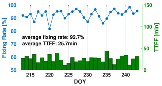
Figure 4.
The ambiguity fixing rates and TTFF of Sentinel-3A real-time POD for DOY 213–243, 2018.
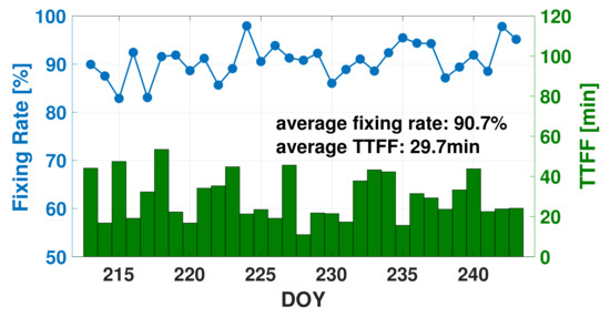
Figure 5.
The ambiguity fixing rates and TTFF of Swarm-A real-time POD for DOY 213–243, 2018.
Generally, the majority of LEO missions are on altitudes of 300–1500 km. Below that level, a satellite’s orbit would rapidly decay due to the strong drag of the Earth’s atmosphere while the higher altitude is abandoned because of the impact of Van Allen Radiation Belts. As a result, the GNSS signals from GNSS satellites to LEO receivers won’t pass through the troposphere in most cases. The troposphere delay is thus ignored in the POD process. It contributes to an increase in the observation redundancy because of the reduction of estimated parameters, yielding a stronger solution strength. Moreover, considering that the LEO satellite’s orbital velocity is 3–7 km/s, the relative motion between the LEO and GNSS satellites would change much more rapidly than that of ground receivers, which leads to a relatively better geometry diversity for LEO POD. As a result, the multipath effects of LEO receivers would be mitigated effectively and the convergence time would be shortened in POD [15]. However, as the side effect of the high dynamic, the signal passes (continuous tracking arcs) of LEO receivers are usually only around 15 min, which may hamper the NL ambiguity fixing [25].
4.2. POD Results
In order to investigate the performance of proposed POD method, both the ambiguity–fixed solution and ambiguity–float solution are assessed from the following three aspects:
- Differences with reference orbit products;
- SLR residuals;
- Carrier phase residuals.
For the orbit difference comparison, the post-processed reduced dynamic orbit products from ESA are adopted as the reference orbits. This is because the kinematic orbits usually present inferior precisions than those of reduced dynamic orbits due to the absence of dynamical constraints [30]. Figure 6 exhibits the orbit differences of Sentinel-3A satellite for ambiguity–fixed and ambiguity–float solutions in DOY 214, 2018, 12:00 a.m. to 6:00 a.m. The red dots refer to the ambiguity–fixed solution while the blue ones denote the ambiguity–float solution. For demonstration of the impact of GNSS satellites’ geometric distribution on LEO Kinematic POD, the visible satellite numbers, position dilution of precision (PDOP) values, and the latitude of LEO satellite ground tracks are also displayed. It can be found that the orbit errors of ambiguity–float solution in the along-track and radial components show dramatic and cyclic variations with a peak-to-peak value of approximately 20 cm. A similar phenomenon can also be observed in cross-track components, although it is less significant. Taking the LEO satellite’s latitude into consideration, we can recognize a potential correlation between the latitude change and periodic variation of orbit error: the LEO satellite shows inferior POD accuracy in high latitude while the POD accuracy is relatively better in low altitude. This may be attributed to the relatively less coverage of GNSS constellation in a high-latitude region (GPS satellites’ inclination is approximately ). As depicted in Figure 6, the average PDOP value is 2.16 in middle and low latitudes (latitude < ) while it increases to 2.52 in high latitudes (latitude > ). In addition, due to the absence of dynamic constraint, kinematic orbit precisions are dominated by the observation quality. Thus, in case of observations’ sudden discontinuities and poor geometric distribution, the kinematic orbits usually present short-term systematic errors.
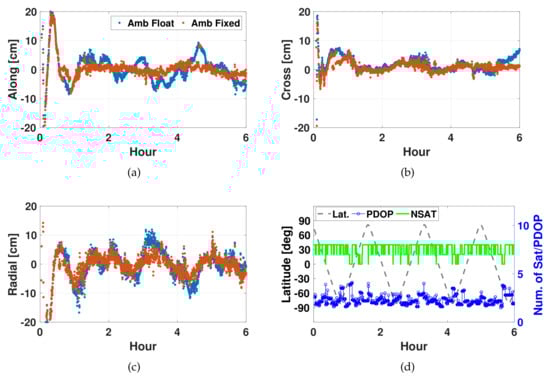
Figure 6.
Orbit differences of the real-time kinematic Sentinel-3A orbit based on comparison with post-processed reduced dynamic orbit: (a) along-track position errors; (b) cross-track position errors; (c) radial position errors; the ambiguity–float solution (blue dots) compared to ambiguity–fixed solution (red dots) on DOY 214 of 2018. The visible satellite numbers, PDOP value, and receiver’s latitude are also presented in (d).
Compared with the float solution, the ambiguity–fixed solution provides a conspicuously smoother variation of the orbit errors. Once the undifferenced phase ambiguities are fixed to their integer values, the estimation would be strengthened immediately, which would offer additional geometric stiffness and ameliorate the orbit accuracy especially near the high latitude area. To mathematically demonstrate the impact of ambiguity fixing on the orbit errors’ cyclic variations, we calculated the Spearman’s correlation coefficients between latitudes of LEO ground tracks and the orbit errors. The statistics are listed in Table 3. Spearman’s correlation coefficient is a statistical measure of the strength of a monotonic relationship between paired data [52]. Unlike Pearson’s correlation, there is no requirement of the parameter’s normality, thus the Spearman’s correlation is more appropriate for the testing of latitudes and orbit errors. For Spearman’s correlation coefficient , the closer is to indicates the stronger the monotonic relationship. In addition, p-value refers to the significance test results. The smaller the p-value is, the more confident we are to believe . As shown in Table 3, the values of ambiguity–float solution are from 0.3 to 0.5 by magnitude, which indicate the moderate level monotonic relationships. After the ambiguity fixing, the value for along-track orbit errors reduces to nearly zero with p-value close to 1, strongly indicating the vanishing of the monotonic relationship. The cross-track orbit errors also show a smaller value by magnitude. However, the radial orbit errors present even a worse value compared with the ambiguity–float result, despite the fact that the ambiguity–fixed orbit error series achieves smaller variations. This is possibly attributed to the poor accuracy in radial components. Overall, the ambiguity fixing alleviates the correlation between orbit errors and latitudes i.e., the satellite geometric conditions. In practical cases, in order to obtain a maximum coverage of the Earth’s surface, the remote sensing satellites are usually injected into the polar or near-polar orbits. The superior performance of ambiguity–fixed solution thus indicates a high potential for improving diverse LEO-based geometric applications. Furthermore, an improvement on convergence time with ambiguity–fixed solution can also be recognized in Figure 6, which is beneficial for the restart after the interrupted tracking in real-time POD.
Table 3.
Spearman’s correlation between latitude and orbit differences for Sentinel-3A.
Figure 7 shows the daily root mean square (RMS) values of real-time kinematic Sentinel-3A orbit differences for the ambiguity–fixed and ambiguity–float solutions. The along-track RMS values for ambiguity–float solution are around 4–6 cm while those for ambiguity–fixed are approximately 3–5 cm. Similar apparent improvement can also be noticed in cross-track and radial component for each day. The detailed statistics are summarized in Table 4. It can be found that the RMS values of Sentinel-3A orbit for the ambiguity–fixed solution are 3.11, 2.19, and 3.59 cm in along-track, cross-track, and radial components, respectively, with an improvement of 30%, 28%, and 23% compared with the ambiguity–float solution. The 3D RMS value decreases from 7.15 cm to 5.23 cm by using ZD AR, which has met the precision requirement of most space missions in real-time situations.
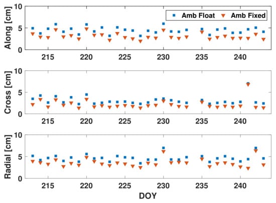
Figure 7.
The daily RMS of Sentinel-3A orbit differences with respect to post-processed reduced dynamic orbit in along-track, cross-track, and radial component, respectively (from top to bottom). The ambiguity–float solution (blue dots) compared to ambiguity–fixed solution (red dots) for DOY 213–243, 2018.
Table 4.
The average RMS values of real-time kinematic Sentinel-3A and Swarm-A orbit differences with different ambiguity strategies.
Orbit differences of Swarm-A satellite in the same period are depicted in Figure 8. Similar to Sentinel-3A, the mean PDOP values increase from 1.83 to 2.11 when the Swarm-A satellite passed the high-latitude areas (latitude > ). Again, the ambiguity–float solution shows evident and periodic variations over the orbital time scale with the peak-to-peak values about 12 cm. The orbit errors of the ambiguity–fixed solution, in the contrast, are remarkably smaller and more stable, particularly in the along-track and cross-track components. In addition, the Spearman’s correlation coefficients between latitudes of LEO ground tracks and the orbit errors for Swarm-A are also summarized. As presented in Table 5, the values for ambiguity–float orbit differences are 0.16 to 0.34, which implies the weak to moderate level monotonic relationships between orbit errors and latitudes. Due to the different orbit inclinations, Swarm-A shows opposite signs of values to Sentinel-3A in the three components: the along-track and radial orbit errors show negative monotonic relationships with latitudes while that of cross-track is positive. In addition, the along-track orbit differences show the strongest correlation while the correlation in radial is the weakest. With the help of ZD AR, the values can achieve 35–75% reductions and add up to around 0.1. Meanwhile, evident increments of p-values are observed. In total, there is strong evidence to prove that the ambiguity fixing can strengthen the parameter estimation and alleviate the orbit errors caused by poor geometric distribution.
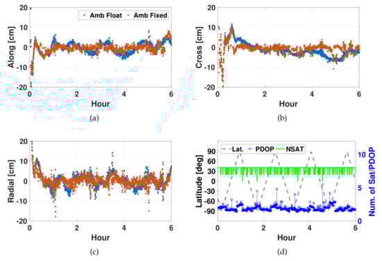
Figure 8.
Orbit differences of the real-time kinematic Swarm-A orbit based on comparison with post-processed reduced dynamic orbit: (a) along-track position errors; (b) cross-track position errors; (c) radial position errors; the ambiguity–float solution (blue dots) compared to ambiguity–fixed solution (red dots) on DOY 214 of 2018. The visible satellite numbers, PDOP value, and receiver’s latitude are also presented in (d).
Table 5.
Spearman’s correlation between latitude and orbit differences for Swarm-A.
The daily RMS values of real-time kinematic Swarm-A orbit are presented in Figure 9. It can be seen that the ambiguity–fixed solution presents a superior POD precision in three components compared with the ambiguity–float solution, with an improvement of around 25%. The 3D RMS value also reduces from 5.29 cm to 4.01 cm as a result of ambiguity resolution. It may be noticed that the Swarm-A orbits achieve 1–2 cm higher accuracy than those of Sentinel-3A. This is probably caused by the absence of Sentinel-3A’s precise attitude information and PCV values.
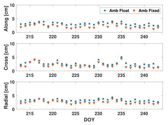
Figure 9.
The daily RMS of Swarm-A orbit differences with respect to post-processed reduced dynamic orbit in along-track, cross-track, and radial component, respectively (from top to bottom), the ambiguity–float solution (blue dots) compared to ambiguity–fixed solution (red dots) for DOY 213–243, 2018.
In addition to the comparison with post-processed reduced dynamic orbit, the ambiguity–fixed orbit and ambiguity–float orbit are also compared against SLR measurements. SLR can provide completely independent optical distance measurements between LEO satellite and ground stations with mm-to-cm-level precision. Thus, SLR residuals, i.e., differences between measured and modeled ranges, serve as a common figure of merit for validation of not only satellite orbits’ precision, but also accuracy [53]. Both Sentinel-3A and Swarm-A are equipped with LRR, and their SLR observations are routinely provided by a worldwide network of the International Laser Ranging Service (ILRS) [54]. However, the equations of motion for orbiting satellites refer to the satellite center of mass (CoM), so a rigorous correction is required to extrapolate the SLR measurements to the CoM. In this experiment, the CoM and LRR position information was from values recommended in [30]. During the study period, the Sentinel-3A satellite was tracked by 17 ILRS stations and those of Swarm-A satellite was 19. Considering that the observation numbers of some ILRS stations are few (less than 50 normal points), two high-performance subsets of ILRS stations are selected for Sentinel-3A and Swarm-A orbit validation, respectively. The corresponding station IDs for Sentinel-3A are 1890, 7090, 7105, 7110, 7501, 7839, 7840, 7841, and 8834, while those for Swarm-A are 7090, 7105, 7237, 7501, 7821, 7825, 7827, 7839, and 7840. In addition, an empirical threshold of 0.2 m was used for deleting outliers in SLR validation.
SLR residuals for Sentinel-3A and Swarm-A are summarized in Table 6 and Table 7. In order to avoid the impact of station-specific ranging biases, the mean and standard deviation values of SLR residuals along with the number of normal points for individual ILRS stations are presented in the tables. For Sentinel-3A, all nine ILRS stations present notable smaller standard deviation values with an ambiguity–fixed solution w.r.t ambiguity–float solution. The reduction of standard deviation values are 0.4–1.8 cm, and the corresponding improvements are 8–40%. Statistics based on the full set of analyzed stations show that the mean and standard deviation values for ambiguity–float solution are −3.26 and 5.07 cm, while the ambiguity–fixed solution counterparts are −2.93 and 4.01 cm, with the standard deviation improvement of 21%.
Table 6.
SLR residuals and number of normal points () for individual ILRS stations employed in the Sentinel-3A orbit validation in August 2018.
Table 7.
SLR residuals and number of normal points () for individual ILRS stations employed in the Swarm-A orbit validation in August 2018.
Superior performances of ambiguity–fixed solution are also observed for Swarm-A SLR residuals. As presented in Table 7, the ambiguity–fixed solution shows evident improvements in the standard deviation values for all the IRLS stations compared with the ambiguity–float solution. The improvements are most pronounced for station 7105, 7821, and 7827, whose standard deviation values reduce by 1–2 cm as a result of ambiguity fixing. The overall standard deviation value of ambiguity–fixed solution is 2.78 cm, with an improvement of 21% compared with the 3.53 cm of ambiguity–float solution. In addition, the overall mean value of SLR residuals also decreases by 0.7 cm in magnitude. The SLR residuals validate that ambiguity fixing could achieve not only higher precision, but also higher accuracy LEO orbit compared with ambiguity–float solution.
Apart from the assessment of LEO orbit precisions, the phase residuals are also analyzed to illustrate the impact of ZD AR on LEO POD. When the phase ambiguities are fixed to integer values, the observation equation and model precision will be notably strengthened. In this way, the integer phase ambiguities will be forcibly separated from other linear-correlated parameters and unmodeled errors, which used to be assimilated into float ambiguity estimates. As a consequence, the phase residuals will increase unavoidably. As exhibited in Figure 10, the RMS values of Sentinel-3A phase residuals for the ambiguity–fixed solutions are 0.5–1.0 mm larger than those of the ambiguity–float solutions for each day. The analogous phenomenon can also be found in Figure 11 for Swarm-A, the averaged RMS values of phase residuals are 6.33 mm for the ambiguity–float solution, while it is 6.79 mm for the ambiguity–fixed solution.
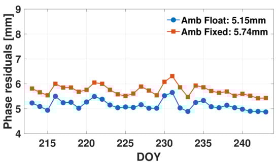
Figure 10.
Daily RMS values of Sentinel-3A phase residuals for DOY 213–243, 2018 with ambiguity–float and ambiguity–fixed solutions.
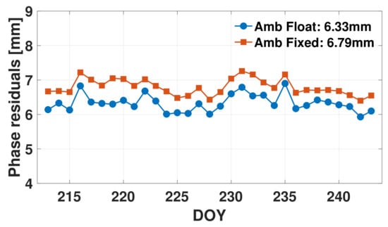
Figure 11.
Daily RMS values of Swarm-A phase residuals for DOY 030–090, 2017 with ambiguity–float and ambiguity–fixed solutions.
5. Discussion
This contribution aims at investigating the performance of real-time kinematic LEO POD with ZD AR based on the onboard GPS measurements. In the proposed method, we firstly estimate the zero-differenced UPDs in real-time processing by making use of real-time GNSS orbit/clock products and observations from a global distributed network. Then, in LEO kinematic POD processing, the zero-differenced ambiguity resolution is performed epoch by epoch with the help of obtained UPD products.
For the assessment of the proposed method, the kinematic Sentinel-3A and Swarm-A POD were performed in simulated real-time situation with ambiguity–fixed and ambiguity–float solutions, respectively. The experiment time span is from 1 August 2018 to 1 September 2018. Firstly, the ambiguity fixing performance is analyzed to confirm the reliability of ZD AR. In the given example, the WL and NL ambiguity residuals, i.e., the UPD-corrected ambiguity subtracting its nearest integer, show distributions that are concentrated to around zero with over 90% and 93% of them less than 0.15 cycles by magnitude. The ambiguity residual distributions indicate the high quality of the estimated real-time WL and NL UPDs. Over the experiment period, the mean ambiguity fixing rate of Sentinel-3A is 92.7% with the mean TTFF of 25.7 min. The corresponding results of Swarm-A is 90.3% and 30 min, respectively. The results demonstrate that the ZD ambiguities of LEO POD can be fixed to proper integer values within a short initialization period with high reliability.
As for the POD performance, both Sentinel-3A and Swarm-A achieve notable improvements with the help of ZD AR. Overall, 27% and 16% precision improvements can be observed for Sentinel-3A and Swarm-A in terms of the orbit difference with final products. Due to the absence of dynamic constraint, the orbit errors of the float solution show dramatic variations over the orbital period especially when the LEO satellite passes high-latitude areas, where the coverage of GNSS constellations is relatively less. By fixing the phase ambiguities to integer values, extra geometric stiffness would be provided and the parameter estimation is thus strengthened. This explains the reason why ambiguity–fixed solutions show conspicuous smoother variations of the orbit errors compared with ambiguity–float solutions. Here, the Spearman’s correlation coefficient () is introduced to mathematically describe the impact of ZD AR on the cyclic variation of orbit errors. From the results between latitudes of LEO ground tracks and orbit errors, we can see a weak to moderate level monotonic correlation for ambiguity–float solutions. The ambiguity–fixed solution, in contrast, provide evidently smaller values, which indicate that the orbit errors caused by poor geometric distributions have been largely alleviated. In addition, the convergence time of orbit errors also benefits from the ZD AR, which is helpful to cope with the interrupted tracking in real-time POD. The accuracy of kinematic Sentinel-3A and Swarm-A orbits is further validated with SLR measurements. The standard deviation of Sentinel-A SLR residuals is 3.9 cm using an ambiguity–fixed solution, with an improvement of 22% compared with the ambiguity–float solution. A similar improvement of 15% is achieved for Swarm-A likewise.
After fixing the ZD ambiguities to integer values, the integer ambiguities will separate from the unmodeled errors that used to be absorbed in float solution. As a consequence, the phase residuals will increase inevitably. Therefore, the increments of phase residuals can also serve as an indirect index for the impact of ZD AR on LEO POD. When the ambiguity–fixed solution was applied, the Sentinel-3A and Swarm-A phase residuals increased from 5.15 to 5.74 cm and 6.33 to 6.79 cm, respectively. In summary, fixing onboard GPS phase ambiguities to proper integer values is a powerful method to enhance the kinematic LEO orbits in real-time situations.
Author Contributions
Conceptualization and methodology, X.L. (Xingxing Li) and J.W.; software, X.L. (Xingxing Li); validation, J.W., K.Z., X.L. (Xin Li), and Y.X.; formal analysis, J.W., X.L. (Xin Li), and Y.X.; investigation, X.L. (Xingxing Li), J.W., and K.Z.; resources, X.L. (Xingxing Li), K.Z., and Q.Z.; data curation, X.L. (Xingxing Li), J.W., Q.Z.; writing—original draft preparation, J.W.; writing—review and editing, X.L. (Xingxing Li), K.Z., and X.L. (Xin Li); visualization, J.W.; supervision, X.L. (Xingxing Li); project administration, X.L. (Xingxing Li); funding acquisition, X.L. (Xingxing Li).
Funding
This study is financially supported by the National Natural Science Foundation of China (Grant No. 41774030, No. 41974027, No. 41974029), and the HuBei Province Natural Science Foundation of China (Grant No. 2018CFA081).
Acknowledgments
We are very grateful to ESA for providing the raw GNSS observations and post-processed reduced dynamic orbit of Sentinel-3A and Swarm-A. The Sentinel-3A GNSS observations are available from https://scihub.copernicus.eu/gnss, and the orbit products can be found on https://sentinels.copernicus.eu/web/sentinel/missions/sentinel-3/ground-segment/pod/products-requirements. Swarm-A data are publicly available from ftp://swarm-diss.eo.esa.int. Thanks also go to the EPOS-RT/PANDA software from Deutsches GeoForschungsZentrum (GFZ), Potsdam, Germany. The numerical calculations have been done on the supercomputing system in the Supercomputing Center of Wuhan University. Finally, we thank anonymous reviewers for their helpful comments, which helped us improve the manuscript.
Conflicts of Interest
The authors declare no conflict of interest. The funders had no role in the design of the study; in the collection, analyses, or interpretation of data; in the writing of the manuscript, or in the decision to publish the results.
Abbreviations
The following abbreviations are used in this manuscript:
| AR | Ambiguity Resolution |
| BDS | BeiDou Navigation Satellite System |
| CLS | Collecte Localisation Satellites |
| CNES | Centre National d’ Etudes Spatiales |
| CoM | Center of Mass |
| CODE | Center for Orbit Determination in Europe |
| COSMIC | Constellation Observing System for Meteorology Ionosphere and Climate |
| CSES | China Seismo-Electromagnetic Satellite |
| DCB | Differential Code Bias |
| DD | Double Differenced |
| DORIS | Doppler Orbit determination and Radio-positioning Integrated on Satellite |
| DOY | Day of Year |
| ESA | European Space Agency |
| GLONASS | GLObal Navigation Satellite System |
| GNSS | Global Navigation Satellite System |
| GPS | Global Positioning System |
| HOI | High-Order Ionospheric |
| IF | Ionosphere free |
| IGS | International GNSS Service |
| ILRS | International Laser Ranging Service |
| IRC | Integer Recovered Clock |
| LAMBDA | Least-squares AMBiguity Decorrelation Adjustment |
| LEO | Low Earth Orbit |
| LRR | Laser Retro-Reflector |
| LTAN | Local Time of Ascending Node |
| LTDN | Local Time of Descending Node |
| MGEX | IGS Multi-GNSS EXperiment |
| MW | Melbourne–Wubbena |
| NL | Narrow-Lane |
| NRT | Near-Real-Time |
| NTC | Non Time Critical |
| PCO | Phase Center Offset |
| PCV | Phase Center Variation |
| PDOP | Position Dilution of Precision |
| POD | Precise Orbit Determination |
| PPP | Precise Point Positioning |
| RTS | Real-Time Service |
| SLR | Satellite Laser Ranging |
| STC | Short Time Critical |
| TTFF | Time To First Fix |
| UPD | Uncalibrated Phase Delay |
| WL | Wide-Lane |
| ZD | Zero Differenced |
References
- Bezděk, A.; Sebera, J.; Klokočník, J.; Kosteleckỳ, J. Gravity field models from kinematic orbits of CHAMP, GRACE and GOCE satellites. Adv. Space Res. 2014, 53, 412–429. [Google Scholar] [CrossRef]
- Guo, X.; Zhao, Q. A New Approach to Earth’s Gravity Field Modeling Using GPS-Derived Kinematic Orbits and Baselines. Remote. Sens. 2019, 11, 1728. [Google Scholar] [CrossRef]
- Jäggi, A.; Dahle, C.; Arnold, D.; Bock, H.; Meyer, U.; Beutler, G.; van den IJssel, J. Swarm kinematic orbits and gravity fields from 18 months of GPS data. Adv. Space Res. 2016, 57, 218–233. [Google Scholar] [CrossRef]
- Beckley, B.; Lemoine, F.; Luthcke, S.; Ray, R.; Zelensky, N. A reassessment of global and regional mean sea level trends from TOPEX and Jason-1 altimetry based on revised reference frame and orbits. Geophys. Res. Lett. 2007, 34. [Google Scholar] [CrossRef]
- Cerri, L.; Berthias, J.; Bertiger, W.; Haines, B.; Lemoine, F.; Mercier, F.; Ries, J.C.; Willis, P.; Zelensky, N.; Ziebart, M. Precision orbit determination standards for the Jason series of altimeter missions. Mar. Geod. 2010, 33, 379–418. [Google Scholar] [CrossRef]
- Kursinski, E.; Hajj, G.; Schofield, J.; Linfield, R.; Hardy, K.R. Observing Earth’s atmosphere with radio occultation measurements using the Global Positioning System. J. Geophys. Res. Atmos. 1997, 102, 23429–23465. [Google Scholar] [CrossRef]
- Kang, Z.; Tapley, B.; Bettadpur, S.; Ries, J.; Nagel, P.; Pastor, R. Precise orbit determination for the GRACE mission using only GPS data. J. Geod. 2006, 80, 322–331. [Google Scholar] [CrossRef]
- Wang, F.; Gong, X.; Sang, J.; Zhang, X. A novel method for precise onboard real-time orbit determination with a standalone GPS receiver. Sensors 2015, 15, 30403–30418. [Google Scholar] [CrossRef]
- Montenbruck, O.; Ramos-Bosch, P. Precision real-time navigation of LEO satellites using global positioning system measurements. GPS Solut. 2008, 12, 187–198. [Google Scholar] [CrossRef]
- Hadas, T.; Bosy, J. IGS RTS precise orbits and clocks verification and quality degradation over time. GPS Solut. 2015, 19, 93–105. [Google Scholar] [CrossRef]
- Montenbruck, O.; Hauschild, A.; Andres, Y.; von Engeln, A.; Marquardt, C. (Near-) real-time orbit determination for GNSS radio occultation processing. GPS Solut. 2013, 17, 199–209. [Google Scholar] [CrossRef]
- Strugarek, D.; Sośnica, K.; Jäggi, A. Characteristics of GOCE orbits based on Satellite Laser Ranging. Adv. Space Res. 2019, 63, 417–431. [Google Scholar] [CrossRef]
- Švehla, D.; Rothacher, M. Kinematic precise orbit determination for gravity field determination. In A Window on the Future of Geodesy; Springer: Berlin, Germany, 2005; pp. 181–188. [Google Scholar]
- de Selding, P.B. SpaceX to Build 4000 Broadband Satellites in Seattle. Space News Website, 2015; Volume 19. Available online: http://spacenews.com/spacex-opening-seattle-plant-to-build-4000-broadband-satellites/ (accessed on 19 January 2015).
- Li, X.; Ma, F.; Li, X.; Lv, H.; Bian, L.; Jiang, Z.; Zhang, X. LEO constellation-augmented multi-GNSS for rapid PPP convergence. J. Geod. 2019, 93, 749–764. [Google Scholar] [CrossRef]
- Li, M.; Li, W.; Shi, C.; Jiang, K.; Guo, X.; Dai, X.; Meng, X.; Yang, Z.; Yang, G.; Liao, M. Precise orbit determination of the Fengyun-3C satellite using onboard GPS and BDS observations. J. Geod. 2017, 91, 1313–1327. [Google Scholar] [CrossRef]
- Lin, J.; Shen, X.; Hu, L.; Wang, L.; Zhu, F. CSES GNSS ionospheric inversion technique, validation and error analysis. Sci. China Technol. Sci. 2018, 61, 669–677. [Google Scholar] [CrossRef]
- Svehla, D.; Rothacher, M. Kinematic and reduced dynamic precise orbit determination of low Earth orbiters. Adv. Geosci. 2003, 1, 47–56. [Google Scholar] [CrossRef]
- Montenbruck, O.; Hackel, S.; van den Ijssel, J.; Arnold, D. Reduced dynamic and kinematic precise orbit determination for the Swarm mission from 4 years of GPS tracking. GPS Solut. 2018, 22, 79. [Google Scholar] [CrossRef]
- Blewitt, G. Carrier phase ambiguity resolution for the Global Positioning System applied to geodetic baselines up to 2000 km. J. Geophys. Res. Solid Earth 1989, 94, 10187–10203. [Google Scholar] [CrossRef]
- Bertiger, W.; Desai, S.D.; Haines, B.; Harvey, N.; Moore, A.W.; Owen, S.; Weiss, J.P. Single receiver phase ambiguity resolution with GPS data. J. Geod. 2010, 84, 327–337. [Google Scholar] [CrossRef]
- Ge, M.; Gendt, G.; Rothacher, M.a.; Shi, C.; Liu, J. Resolution of GPS carrier-phase ambiguities in precise point positioning (PPP) with daily observations. J. Geod. 2008, 82, 389–399. [Google Scholar] [CrossRef]
- Li, X.; Zhang, X. Improving the estimation of uncalibrated fractional phase offsets for PPP ambiguity resolution. J. Navig. 2012, 65, 513–529. [Google Scholar] [CrossRef]
- Collins, P. Isolating and estimating undifferenced GPS integer ambiguities. In Proceedings of the Institute of Navigation, National Technical Meeting, San Diego, CA, USA, 28–30 January 2008; pp. 720–732. [Google Scholar]
- Laurichesse, D.; Mercier, F.; BERTHIAS, J.P.; Broca, P.; Cerri, L. Integer ambiguity resolution on undifferenced GPS phase measurements and its application to PPP and satellite precise orbit determination. Navigation 2009, 56, 135–149. [Google Scholar] [CrossRef]
- Loyer, S.; Perosanz, F.; Mercier, F.; Capdeville, H.; Marty, J.C. Zero-difference GPS ambiguity resolution at CNES–CLS IGS Analysis Center. J. Geod. 2012, 86, 991–1003. [Google Scholar] [CrossRef]
- Katsigianni, G.; Loyer, S.; Perosanz, F.; Mercier, F.; Zajdel, R.; Sośnica, K. Improving Galileo orbit determination using zero-difference ambiguity fixing in a Multi-GNSS processing. Adv. Space Res. 2019, 63, 2952–2963. [Google Scholar] [CrossRef]
- Geng, J.; Meng, X.; Dodson, A.H.; Teferle, F.N. Integer ambiguity resolution in precise point positioning: method comparison. J. Geod. 2010, 84, 569–581. [Google Scholar] [CrossRef]
- Shi, J.; Gao, Y. A comparison of three PPP integer ambiguity resolution methods. GPS Solut. 2014, 18, 519–528. [Google Scholar] [CrossRef]
- Montenbruck, O.; Hackel, S.; Jäggi, A. Precise orbit determination of the Sentinel-3A altimetry satellite using ambiguity–fixed GPS carrier phase observations. J. Geod. 2018, 92, 711–726. [Google Scholar] [CrossRef]
- Allende-Alba, G.; Montenbruck, O.; Hackel, S.; Tossaint, M. Relative positioning of formation-flying spacecraft using single-receiver GPS carrier phase ambiguity fixing. GPS Solut. 2018, 22, 68. [Google Scholar] [CrossRef]
- Hofmann-Wellenhof, B.; Lichtenegger, H.; Wasle, E. GNSS–Global Navigation Satellite Systems: GPS, GLONASS, Galileo, and More; Springer Science & Business Media: Berlin, Germany, 2007. [Google Scholar]
- Li, X.; Ge, M.; Dai, X.; Ren, X.; Fritsche, M.; Wickert, J.; Schuh, H. Accuracy and reliability of multi-GNSS real-time precise positioning: GPS, GLONASS, BeiDou, and Galileo. J. Geod. 2015, 89, 607–635. [Google Scholar] [CrossRef]
- Kouba, J. A Guide to Using International GNSS Service (IGS) Products. 2009. Available online: http://igscb.jpl.nasa.gov/igscb/resource/pubs/UsingIGSProductsVer21.pdf (accessed on 18 October 2019).
- Van Den IJssel, J.; Encarnação, J.; Doornbos, E.; Visser, P. Precise science orbits for the Swarm satellite constellation. Adv. Space Res. 2015, 56, 1042–1055. [Google Scholar] [CrossRef]
- Jäggi, A.; Bock, H.; Meyer, U.; Beutler, G.; van den IJssel, J. GOCE: Assessment of GPS-only gravity field determination. J. Geod. 2015, 89, 33–48. [Google Scholar] [CrossRef]
- Zhang, K.; Li, X.; Xiong, C.; Meng, X.; Li, X.; Yuan, Y.; Zhang, X. The Influence of Geomagnetic Storm of 7–8 September 2017 on the Swarm Precise Orbit Determination. J. Geophys. Res. Space Phys. 2019, 124, 6971–6984. [Google Scholar] [CrossRef]
- Melbourne, W. The Case for Ranging in GPS Based Geodetic Systems. In Proceedings of the 1st International Symposium on Precise Positioning with the Global Positioning System, Rockville, MD, USA, 15–19 April 1985; US Department of Commerce: Washington, DC, USA, 1985; pp. 373–386. [Google Scholar]
- Wubbena, G. Software developments for geodetic positioning with GPS using TI 4100 code and carrier measurements. In Proceedings of the 1st International Symposium on Precise Positioning with the Global Positioning System, Rockville, MD, USA, 15–19 April 1985; US Department of Commerce: Washington, DC, USA, 1985; pp. 403–412. [Google Scholar]
- Li, X.; Li, X.; Yuan, Y.; Zhang, K.; Zhang, X.; Wickert, J. Multi-GNSS phase delay estimation and PPP ambiguity resolution: GPS, BDS, GLONASS, Galileo. J. Geod. 2018, 92, 579–608. [Google Scholar] [CrossRef]
- Teunissen, P.; Joosten, P.; Tiberius, C. Geometry-free ambiguity success rates in case of partial fixing. In Proceedings of the 1999 National Technical Meeting of The Institute of Navigation, San Diego, CA, USA, 25–27 January 1999; pp. 25–27. [Google Scholar]
- Li, X.; Chen, X.; Ge, M.; Schuh, H. Improving multi-GNSS ultra-rapid orbit determination for real-time precise point positioning. J. Geod. 2019, 93, 45–64. [Google Scholar] [CrossRef]
- Li, P.; Zhang, X. Precise point positioning with partial ambiguity fixing. Sensors 2015, 15, 13627–13643. [Google Scholar] [CrossRef]
- Ming, W.; Klaus-Peter, S. Fast Ambiguity Resolution Using an Integer Nonlinear Programming Method. In Proceedings of the 8th International Technical Meeting of the Satellite Division of The Institute of Navigation (ION GPS 1995), Palm Springs, CA, USA, 12–15 September 1995; pp. 1101–1110. [Google Scholar]
- Han, S. Quality-control issues relating to instantaneous ambiguity resolution for real-time GPS kinematic positioning. J. Geod. 1997, 71, 351–361. [Google Scholar] [CrossRef]
- Lu, C.; Zhang, Q.; Zhang, K.; Zhu, Y.; Zhang, W. Improving LEO precise orbit determination with BDS PCV calibration. GPS Solut. 2019, 23, 109. [Google Scholar] [CrossRef]
- Wu, J.T.; Wu, S.C.; Hajj, G.A.; Bertiger, W.I.; Lichten, S.M. Effects of antenna orientation on GPS carrier phase. Astrodynamics 1991, 18, 1647–1660. [Google Scholar]
- Friis-Christensen, E.; Lühr, H.; Knudsen, D.; Haagmans, R. Swarm—An Earth observation mission investigating geospace. Adv. Space Res. 2008, 41, 210–216. [Google Scholar] [CrossRef]
- Donlon, C.; Berruti, B.; Mecklenberg, S.; Nieke, J.; Rebhan, H.; Klein, U.; Buongiorno, A.; Mavrocordatos, C.; Frerick, J.; Seitz, B.; et al. The Sentinel-3 Mission: Overview and status. In Proceedings of the 2012 IEEE International Geoscience and Remote Sensing Symposium, Munich, Germany, 22–27 July 2012; pp. 1711–1714. [Google Scholar]
- Feng, Y.; Wang, J. GPS RTK performance characteristics and analysis. J. Glob. Position. Syst. 2008, 7, 1–8. [Google Scholar] [CrossRef]
- Gao, W.; Gao, C.; Pan, S.; Wang, D.; Deng, J. Improving ambiguity resolution for medium baselines using combined GPS and BDS dual/triple-frequency observations. Sensors 2015, 15, 27525–27542. [Google Scholar] [CrossRef] [PubMed]
- Spearman, C. The Proof and Measurement of Association between Two Things. Am. J. Psychol. 1904, 15, 72–101. [Google Scholar] [CrossRef]
- Arnold, D.; Montenbruck, O.; Hackel, S.; Sośnica, K. Satellite laser ranging to low Earth orbiters: Orbit and network validation. J. Geod. 2018, 1–20. [Google Scholar] [CrossRef]
- Pearlman, M.R.; Degnan, J.J.; Bosworth, J. The international laser ranging service. Adv. Space Res. 2002, 30, 135–143. [Google Scholar] [CrossRef]
© 2019 by the authors. Licensee MDPI, Basel, Switzerland. This article is an open access article distributed under the terms and conditions of the Creative Commons Attribution (CC BY) license (http://creativecommons.org/licenses/by/4.0/).