Abstract
Urban expansion results in landscape pattern changes and associated changes in land surface temperature (LST) intensity. Spatial patterns of urban LST are affected by urban landscape pattern changes and seasonal variations. Instead of using LST change data, this study analysed the variation of LST aggregation which was evaluated by hotspot analysis to measure the spatial dependence for each LST pixel, indicating the relative magnitudes of the LST values in the neighbourhood of the LST pixel and the area proportion of the hotspot area to gain new insights into the thermal effects of increasing impervious surface area (ISA) caused by urbanization in Fuzhou, China. The spatio-temporal relationship between urban landscape patterns, hotspot locations reflecting urban land cover change in space and the thermal environment were analysed in different sectors. The linear spectral unmixing method of fully constrained least squares (FCLS) was used to unmix the bi-temporal Landsat TM/OLI imagery to derive subpixel ISA and the accuracy of the percent ISA was assessed. Then, a minimum change threshold was chosen to remove random noise, and the change of ISA between 2000 and 2016 was analysed. The urban area was divided into three circular consecutive urban zones in the cardinal directions from the city centre and each circular zone was further divided into eight segments; thus, a total of 24 spatial sectors were derived. The LST aggregation was analysed in different directions and urban segments and hotspot density was further calculated based on area proportion of hotspot areas in each sector. Finally, variations of mean normalized LST (NLST), area proportion of ISA, area proportion of ISA with high LST, and area proportion of hotspot area were quantified for all sectors for 2000 and 2016. The four levels of hotspot density were classified for all urban sectors by proportional ranges of 0%–25%, 25%–50%, 50%–75% and 75%–100% for low-, medium-, sub-high, and high density, and the spatial dynamics of hotspot density between the two dates showed that urbanization mainly dominated in sectors south–southeast 2 (SSE2), south–southwest 2 (SSW2), west–southwest 2 (WSW2), west–northwest 2 (WNW2), north–southwest 2 (NSW2), south–southeast 3 (SSE3) and south–southwest 3 (SSW3). This paper suggests a methodology for characterizing the urban thermal environment and a scientific basis for sustainable urban development.
1. Introduction
Urban areas play an important role in adapting to and mitigating climate change [1,2]. Urbanization that converts pervious surfaces (such as grassland, forests, water bodies, crop fields, etc.) into impervious surfaces leads to variations in microclimate that impact human health and the urban environment [3,4,5]. As urbanization accelerates, there is growing interest in understanding its implications on climatic change and further garners considerable attention to mitigate the urban heat island (UHI) effect [6,7,8].
Land surface temperature (LST) is an important parameter for the study of the urban heat island phenomenon and environmental change [9,10,11,12]. Urban LST is higher and more variable than concurrent air temperatures due to the spatial heterogeneity of land cover types, variations of urban topography, building layout, building density and other factors [13,14,15]; therefore, LST is affected by urban land cover types and their composition and configuration [16,17]. The LST from Landsat sensors is often used to analyse spatial and temporal relationships between the urban thermal environment, land cover and landscape pattern [13,18,19,20]. The relationship between LST and vegetation index is usually analysed to differentiate surface properties and reveal the pixels ranging from low temperature for high vegetation cover to high temperature for low vegetation cover as an effect of the urbanization process [21,22,23,24]. Impervious surface area (ISA) data have been used in combination with vegetation indices to characterize LST differences [25,26]. The percent of ISA data, which estimates the relative amount of impenetrable surface, is used to study the urban thermal environment because of strong positive correlations with LST [27,28,29,30,31,32,33].
The high spectral variations of urban pixels make it difficult to classify urban land cover accurately with per-pixel classifiers [34,35]. Therefore, traditional per-pixel classifiers cannot effectively handle the complex fine-scale urban landscape patterns due to the mixed pixel problem. Urban biophysical parameters such as Normalized Difference Vegetation Index (NDVI), Enhanced Vegetation Index (EVI), Normalized Difference Built-up Index (NDBI) and Normalized Difference Bareness Index (NDBaI) have widely been used to analyse their relationships with remotely sensed LST and further describe the UHI phenomenon [28,36,37]. Sub-pixel land cover types are usually extracted by spectral unmixing and percent ISA from 0%–100% can reveal varying densities and patterns of urban areas [38,39]. The LST within urban areas is not homogenous but interrupted by high or cold LST spots associated with areas of high or low fractional ISA [40,41]. Hence, more research is needed to study the impacts of ISA changes on the urban thermal environment based on different areas such as the urban core, community areas, industrial areas, etc., because cities expand differently in different areas. In order to develop effective climate change adaptation strategies in urban environments, it is necessary to analyse LST and urban landscape patterns in different sectors and directions of urban expansion as an alternative approach to previous urban thermal environment analysis [39,42].
Instead of analysing the relationships between vegetation indices with LST, this study focused on the impact of urban percent ISA on LST clusters in different sectors. The spatial distribution of urban LST hotspots has a significant impact on human health and comfort and is essential for sustainable urban planning [3,43]. This study attempts to analyse the directional distributions of LST clustering and urban expansion by incorporating bi-temporal LST aggregation change data with spatial statistics. This study differs from previous studies in two aspects. First, the spatial patterns of the hotspot densities were used to analyse urban land cover transformation and the thermal environment. Second, the direction and magnitude of the urban expansion effect were delineated by the proportion of hotspot areas and percent ISA when the whole urban area was classified into different angular sectors.
The objectives of this study were to (1) interpret urban land cover transformations with LST clusters and ISA and to (2) quantify the spatial pattern of the urban thermal environment in different urban segments through LST aggregation densities, analysing the direction of urban expansion.
Fuzhou, the capital city of Fujian Province, China, was selected as the study area, and two Landsat images acquired on 29 June 2000 and 27 July 2016 were selected to quantify the urban landscape patterns and the thermal environment.
2. Materials and Methods
2.1. Study Area and Data
The study area, located on the southeast coast of China, is shown in Figure 1. Fuzhou has experienced rapid urban expansion over the last 20 years, with a population of about 6.5 million in 2000 and 7.5 million in 2016. Affected by the physical geographical environment, economic growth and population growth, urban planning, transportation, etc., the urban expansion of Fuzhou has varied in different areas and directions.
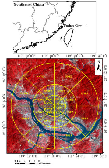
Figure 1.
The study area of Fuzhou as a false-colour composite of a Landsat 8 Operational Land Imager (OLI) image (bands 432) in RGB acquired on 27 July 2016 (the study area was divided into different sectors from city centre to urban peripheral areas by the yellow lines in the figure which are further illustrated in Section 2.2.4).
The city has a subtropical humid climate and the vegetation cover in the region is predominantly evergreen with almost no seasonal variations. The weather of Fuzhou in spring, autumn and winter is relatively cool and the weather variations between spring, autumn and winter are not as large. The summers, however, are very hot with an average of 37.5 days of temperatures exceeding 35 °C. Therefore, in order to reduce the effect of seasonal variations, two Landsat images were selected to quantify the spatial-temporal distributions of urban landscape patterns and the thermal environment (Table 1). In order to assess the accuracy of subpixel land cover type derivation, high-resolution IKONOS and GeoEye-1 images, acquired close to the dates of the corresponding Landsat TM/OLI images, were also used (Table 1). All data were georeferenced to a common Universal Transverse Mercator coordinate system based on the geocoded high-resolution IKONOS image. The root mean square error (RMSE) of the georectification of the Landsat data was <0.3 pixels.

Table 1.
Landsat and high-resolution images of the study area.
2.2. Methods
The methodology for this research consisted of four main steps. Step 1 involved fractional cover derivation, Landsat LST retrieval, and LST classification. Step 2 involved urban landscape pattern analysis based on sectors. Step 3 delineated the spatial aggregation of LST in different urban sectors related to urban development density and direction through LST hotspot analysis. Step 4 explored the bi-temporal impervious surface change and its impact on thermal environment through analysing the relationships between mean normalized LST (NLST), percent ISA, the area ratio of ISA with high LST, area ratio of hotspot area in each sector, and classification of hotspot densities based on the areal ration of the hot spot area at each sector.
2.2.1. Land Surface Temperature Retrieval and Grading
The LST was retrieved from the Landsat data by the radiative transfer equation in the study. Firstly, the digital numbers of the bands were converted to top-of-atmosphere (TOA) radiance through radiometric calibration. Secondly, the TOA radiance of visible/near-infrared bands and thermal band were respectively converted to surface reflectance and surface-leaving radiance by atmospheric correction using the radiative transfer code MODTRAN [44,45]. The surface-leaving radiance LT is calculated with Equation (1) [46]:
where Lμ, τ and Ld, respectively, are the upwelling radiance, atmospheric transmission and downwelling radiance retrieved through atmospheric correction. ε is the emissivity calculated based on the NDVI and land cover types [47,48]. The NDVI was calculated based on the surface reflectance of bands 3 (red band) and 4(near-infrared band) of the Landsat images. In Equation (1), Lλ is the TOA radiance image of the thermal infrared band.Because the larger uncertainty existed in the thermal infrared band 11 values, the thermal infrared band 10 was recommended to derive LST for Landsat 8 (http://landsat.usgs.gov/Landsat8_Using_Product.php). Therefore, single spectral band 10 data were used to retrieve the LST in this study as that for the LST retrieval of Landsat TM/ETM+.
LT = (Lλ− Lμ − τ (1 − ε)Ld)/τ ε
Finally, the radiance LT was converted to surface temperature using Equation (2) [49]:
where LST is the temperature in Kelvin (K) andk1 and k2 are the pre-launch calibration constants respectively in W/(m2.sr/μm) and Kelvin. For Landsat 5 TM, k1 = 607.76W/(m2.sr.μm) and k2= 1260.56 K. For TIRS band 10, k1 = 774.89W/(m2.sr.μm) and k2= 1321.08 K. The LST from the TIRS image with spatial resolution of 100 m was resampled to 120 m to match the pixel size of the LST from the TM image.
Due to the effect of the seasonality and variability of atmospheric conditions, the LST of a same object will show some differences for different dates. In order to reduce the influence of such LST fluctuations, many researchers divide the LST images into defined temperature ranges [50,51]. In this study, the LST values were subdivided into four different classes by adding or subtracting standard deviation (SD) from its mean. The four LST classes were created using the following standard:
LSTClass 1: LST ≤ (MeanLST − 2SD)
LSTClass 2: (MeanLST − 2SD) < LST ≤ MeanLST
LSTClass 3: MeanLST < LST ≤ (MeanLST + 2SD)
LSTClass 4: LST > (MeanLST + 2SD)
LSTClass 2: (MeanLST − 2SD) < LST ≤ MeanLST
LSTClass 3: MeanLST < LST ≤ (MeanLST + 2SD)
LSTClass 4: LST > (MeanLST + 2SD)
The LST increase from LSTClass 1 to LSTClass 4. The LSTClass 4 area has the highest LST and is defined as a high temperature area. The map of the four LST classes can be used to analyse the evolution of the thermal environment.
The LST values can be scaled between the minimum and maximum LST values to calculate the normalized LST (NLST) to adjust the LST of images acquired at different dates [52]. In this study, the minimum and maximum LST values were identified in each LST image and were further used to calculate the NLST values as follows:
here, LSTmax and LSTmin are minimum and maximum LST values in the LST image respectively.
NLST = (LST − LSTmin)/(LSTmax − LSTmin)
2.2.2. Spectral Unmixing by Fully constrained Least Squares and Accuracy Assessment
In this study, the fully constrained least squares (FCLS) was used to unmix the Landsat TM/OLI imagery. The reflectance of every pixel at each spectral band can be assumed as a linear combination of the reflectances of all endmembers within the pixel and that the spectral proportions of the endmembers represent proportions of the area [53,54,55]. The spectral reflectance in band i can be described as:
where n is the number of endmembers, fk the fraction of endmember k within the pixel, Rik the spectral reflectance of endmember k in band I, and εi the residual error for band i. The fully constrained linear spectral unmixing algorithm results of endmember fractional cover in each pixel must sum to one and must be non-negative. These conditions can be described by Equation (6):
Because the water endmember class is not directly relevant to urban land cover composition, the water surfaces were masked out from the images before spectral unmixing. A variety of methods are used to select endmembers from the image itself [29,56].Yang et al. [57] proved that a triangle was the optimal construction of the spectral scatter plot in a two-dimension spectral mixing space, and the vertices of this triangle should be the optimal three endmembers. In this study, image endmembers were also derived by constructing appropriate two-dimensional spectral mixing spaces.
The spectral characteristics of ISA in urban areas vary widely and impervious surfaces can be represented by high- or low-albedo endmembers [58]. In this study, four endmembers were defined: vegetation, high-albedo impervious surfaces (such as concrete), low-albedo impervious surfaces (such as asphalt), and soil. The high-albedo fraction image also included some bare soil. Because of the spatial distribution of bare soil areas along the river, they did not have a significant effect on the estimation of percent ISA in the city. With the FCLS model, a constrained least squares solution was applied to spectrally unmix four fractional cover images. The high- and low-albedo impervious surfaces were summed to an image of total percent ISA. Because the emphasis here is on the analysis of the transformation from pervious to impervious surface and its impacts on the thermal environment, two fractional cover images of ISA are only shown in Figure 2. The sampled plots delineated with two polygons in Figure 2a were selected on two Landsat summer images for comparing fractional covers derived by spectral unmixing and reference data derived from the high resolution IKONOS/GeoEye-1.
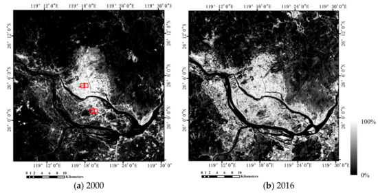
Figure 2.
Fractional impervious surface images generated from FCLS model in 2000 and 2016. (a) Fractional impervious surface in 2000; (b) fractional impervious surface in 2016. The two polygons in (a) represent the test sites used for the accuracy assessment.
As with our previous studies in References [39,42], the accuracy of fractional covers derived from TM/OLI imagery by FCLS was assessed by comparing the fraction estimates in selected test areas with the reference data extracted from the very high-resolution (VHR) IKONOS and GeoEye-1 images. Two test areas in Figure 2a were selected to analyse the accuracy. The iterative self-organizing data analysis technique (ISODATA) was used to extract land cover types from the VHR data, and the test areas were selected as reference data. This approach was feasible because the acquisition dates of IKONOS/GeoEye-1images were very close to the dates of the corresponding TM/OLI imagery. Therefore, the land cover did not change significantly between the IKONOS/GeoEye-1 and TM/OLI imagery.
2.2.3. Characterizing Urban ISA Changes Based on Fractional ISA
The normal method for deriving land cover change from bi-temporal land cover layers is to tabulate class change data between two different dates. This post-classification comparison can result in two problems: (i) errors of each year will propagate into the land cover change map [59,60], (ii) error propagation will lead to inconsistent land cover change results. In this study, the images were converted to atmospherically corrected surface reflectance. In order to analyse ISA change based on fractional ISA, a minimum change threshold was chosen to remove random noise which can arise from image misregistration, atmospheric contamination, varying sun angles and viewing geometry and other factors. The number of pixels was identified as urban expansion changes with the choice of the change threshold of fractional ISA.
Urban expansion is irreversible and urban ISA is rarely converted back to pervious surfaces between two dates [34,61,62,63,64,65]. Hence, urban expansion refers to the expansion of impervious surface cover, and our focus was on impervious cover. Other urban land cover changes, such as the growth of vegetation, were negligible and not assessed.
2.2.4. Zonal and Sectoral Analysis on the Dynamics of Urban Landscape Pattern and LST Aggregation
In order to analyse the spatio-temporal urban landscape patterns and thermal environment in detail, the urban area was divided into three concentric circular zones (Zone 1, Zone 2 and Zone 3) from the city centre by comparing urban area and its expansion in bi-temporal images. Zone 1 was the urban core zone in both years, 2000 and 2016. Zone 3 included mainly peripheral urban areas. Zone 2 was a transition zone between Zone 1 and Zone 3. Zone 2 was not included in the urban area in 2000 and only in the urban area extent of 2016 because of urban expansion. Each of the three circular zones was further divided into eight different directions, thus producing a total of 24 spatial sectors as in Figure 1. The circular zones and sectors were designed in such a way that all radial sections had different directions and different development densities. The data generated from the zonal and sectoral statistics helps in understanding the possible direction of urbanization and related landscape pattern change. Sub-dividing the urban and surrounding rural areas into different sectors enables detailed analysis of the degree of ISA change and spatial LST patterns by incorporating distance and direction as factors. Therefore, it can help in establishing spatial relationships between land cover changes and thermal environmental dynamics as a function of distance and direction from the city centre.
An analysis of the variation of urban landscape patterns and the thermal environment in different sectors was further undertaken by the hotspot analysis. The hotspot analysis tool (Getis-OrdGi*) in ArcGIS was used to explore the aggregation of LST in urban areas and evaluate how thermal aggregation is related to distance from the city centre and change of urban landscape pattern [66]. Unlike directly analysing LST maps, a pixel with a high LST value may not be a statistically significant hotspot. To be a statistically significant hotspot, a pixel must have a high LST value and must be surrounded by other pixels with high LST values. Therefore, the identification of hotspot areas does not depend on whether the value of an LST pixel is high or low. The spatial pattern and statistical significance of LST clustering was evaluated through Getis-OrdGi* as in Equation (7) [67].
where wi,j in Getis-OrdGi* is the spatial weight between features i and j and is calculated based on the Queen’s adjacency connectivity matrix [68], xj is the attribute value for feature j, and n is equal to the total number of features. In this study, hotspot analysis quantitatively analysed the spatial autocorrelation of LST by providing a measure of spatial dependence for each LST pixel and indicating the relative magnitudes of the LST values in the neighbourhood of the LST pixel [69].
3. Results
3.1. Area-Based Accuracy of Fractional Covers
Two test sites (Figure 2a) were selected to assess the accuracy of the total areas by comparing the total area of fractional cover for each land cover type with those estimated from the VHR reference data. Table 2 shows the results from a comparison of the reference area obtained from VHR data with the corresponding area calculated from the Landsat TM/OLI imagery by FCLS.
Table 2.
Results of the accuracy assessment of fractional covers derived by fully constrained least squares (FCLS). Areas measured in km2.
Table 2 indicates good agreement for ISA and vegetation cover between the areas obtained from Landsat and VHR data. Comparing with the reference data, the area of ISA and vegetation in two test sites in 2000 and 2016 shows only small differences. In Table 2, the accuracy of impervious surfaces was slightly lower in 2000 than that in 2016;the difference of ISA derived from TM/OLI imagery and corresponding VHR images was 9.85%in site 1and6.87% in site 2 for 2000 and 7.71% in site 1 and −6.55%in site 2 in 2016, respectively. The accuracy of the vegetation fractions in the two test sites was higher than for ISA at both dates, because the vegetation spectra can be easily distinguished from other land cover types. The accuracy of soil was lower because soil spectra were confused with the high-albedo impervious surfaces. The overall classification accuracy in both cases was less than 11% different between fractional covers of ISA, vegetation, and bare soil derived from TM/OLI imagery and those from VHR images which indicated that the process of fractional cover derivation was reliable. It should be noted that the focus here was not to assess the accuracy of fractional cover by FCLS but rather to provide an insight into the relationships among the change of landscape patterns and its impact on urban thermal environment. The sample areas are representative for the whole study area and provide a good representation of the overall accuracy. Considering the heterogeneity of the urban landscape pattern, the results showed that endmember fractions derived by FCLS are a good representation of reality in the study area.
3.2. ISA and LST Change Based on Different Zones and Sectors
In order to remove random noise in fractional ISA change analysis between 2000 and 2016, a change threshold of 10% fractional ISA was applied. The 10% threshold for fractional ISA change was chosen based on the experimental and empirical analysis in Figure 3. Figure 3 shows the number of pixels identified as fractional ISA changes between 2000 and 2016. The frequency distribution of fractional ISA change suggests a turning point between 10–15%, those less than 10%, especially near 5% fractional ISA change pixels are more likely from random noise, whereas those change pixels more than 10% threshold, especially at the right of the distribution in Figure 3 are likely true ISA change. Those change pixels below 10% threshold are more likely errors, which increase rapidly from 0% to 5% and increase relatively slowly from 5% to 10%. In addition, those pixels with low fractional ISA below 10% are usually difficult to derive accurately by spectral unmixing. Therefore, the 10% change threshold can remove or reduce the noise pixels to some extent in this study.
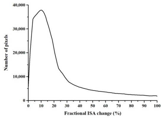
Figure 3.
Number of pixels at fractional impervious surface area (ISA) change of the study area between 2000 and 2016.
Based on the minimum ISA change threshold of 10%, the area variation of ISA was analysed by zones and sectors. Table 3 shows the area and variation of impervious surface in three zones between 2000 and 2016. The study area includes the urban core (Zone 1) of the city, the peripheral urban areas (Zone 3), and a transition Zone 2 between Zone 1 and Zone 3 (Figure 1); Zones 2 and 3 have undergone very high land use alterations due to the urbanization process from 2000 to 2016. Table 3 shows that the area of impervious surface increased from 10.54 km2 to 12.21 km2 in Zone 1, increased from 30.61 km2 to 58.32 km2 in Zone 2, and increased from 52.14 km2 to 140.96 km2 in Zone 3, respectively. The total area of ISA increased by 118.20 km2 from 2000 to 2016. There was a sharp ISA increase in Zone 2 and Zone 3 between the two dates. The area of impervious surface only increased by 15.84% in Zone 1; however, the area of impervious surface increased in Zone 2 by 90.53% and in the new urban development Zone 3 by 170.35% because the fringe of the urban area is the frontier of urban expansion with ISA increase.
Table 3.
The area and areal variation of impervious surface in three zones between 2000 and 2016.
In order to analyse the variations of ISA in more detail, the area of impervious surface was aggregated for eight directions of three zones for both dates. Figure 4 shows a radar chart of the area variation of impervious surface in each sector of the three zones in 2000 and 2016. Figure 4 indicates that the ISA varied in all directions/sectors of the three zones from 2000 to 2016; however, the area of impervious surface increased relatively little, less than 1 km2 in each sector of the urban core Zone 1 (as in Figure 4a, less than 2.0 km2 in all directions as in Table 3). It should be noted that the ISA decreased very little in two directions—ESE1 and SSE1—in Zone 1 between the two dates because urban green spaces attracted more attention in urban planning than urban expansion. Figure 4b shows that ISA increased in all the directions of Zone 2, especially in the direction from WNW2 to SSE2 of Zone 2. Similar to the ISA increase in Zone 2, ISA also increased in all the directions of Zone 3, more strongly than in any direction of Zone 2 (Figure 4c). The ISA increased over 20 km2 in the sectors from the direction WNW3 to ESE3 of Zone 3. Constrained by the mountain located in the north of the study area, ISA increased very little from the direction NNW to ENE in Zone 2 (Figure 4b) and Zone 3 (Figure 4c). The results in Figure 4 not only show the area and its variation of impervious surface in different directions, but also helps to understand the thermal effects of urbanization in different areas of the city.
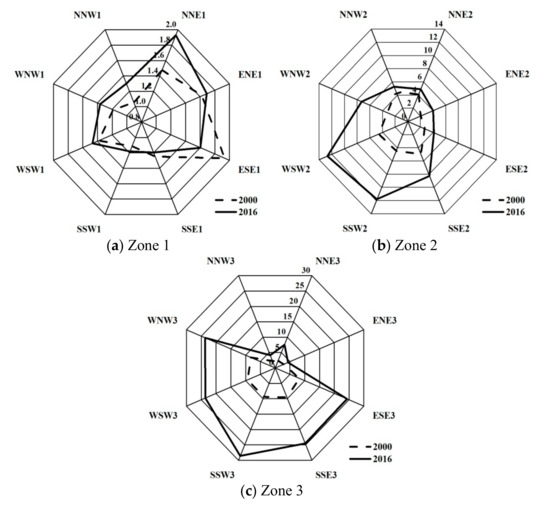
Figure 4.
Area of impervious surface (km2) in each directional sector of three consecutive zones between 2000 and 2016. (a) area of impervious in zone 1; (b); area of impervious in zone 2 (c) area of impervious in zone 3.
In addition to the ISA distribution and change analysis, the spatial heterogeneity of high LST areas was also analysed. Four LST classes were created as in Equation (3) and are shown in Figure 5. The spatial distribution and variation of the highest level LSTareLSTClass4—between 2000 and 2016, which is related to the urbanization process, was further analysed. Compared with three zones in Figure 1, in 2000, the LSTClass 4 was mainly distributed in the city centre (Zone 1), and some areas of Zone 2 were also covered by LSTClass 4. In 2016, except for Zone 1, the LSTClass 4 was distributed in larger parts of Zone 2 and expanded in peripheral Zone 3. In 2000, only some small areas of LSTClass 4 were evident in Zone2, mainly distributed in the south of the transition urban Zone 2. Few LSTClass 4 areas were distributed in the urban peripheral Zone 3 in 2000. However, there was an obvious expansion of the LSTClass 4 from Zone 2 to Zone 3 in 2016 and LSTClass 4 areas were distributed in different directional areas in 2016, which indicates the urban expansion process in which vegetation and agriculture land were replaced by ISA between the two dates to result in high LST areas. Especially in the new urban development Zone 3, a series of discrete high LST areas were formed due to the development of new city areas including the suburb and some newly developed towns from 2000 to 2016.
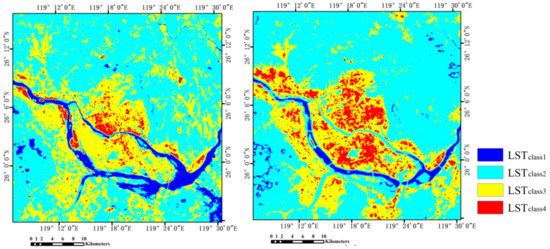
Figure 5.
The spatial distributions of four LST classes for the study area in 2000 and 2016. (a) LST classes in 2000; (b) LST classes in 2016.
3.3. Analysing Spatial and Temporal Pattern of LST Aggregation with Urban Expansion
The hotspot analysis was applied to evaluate the spatial LST clustering that is related to the urban expansion. By providing a measure of spatial dependence for each LST pixel in the neighbourhood of the pixel, the hotspot analysis can characterize the presence of hot spots (high LST clustering) and cold spots (low LST clustering), the thermal aggregation and thermal variation over the study area at different dates [68].
The output of the Getis-OrdGi* statistic returned for each feature in the dataset is a z-score. In this study, higher positive z-score shows clustering of high LST values (hot spot) and a smaller negative z-score represents intense clusters of low LST values (cold spot). The z-score represents the statistical significance of clustering for a specified distance. At a significance level of 0.05 (95%), z-score values >1.96 are statistically significant and chosen to identify areas with significant aggregation of high LST in this study (Figure 6).
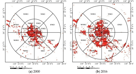
Figure 6.
Hotspot maps showing high LST aggregation in 24 sectors of the study area in 2000 and 2016 (red colour shows hot spot areas). (a) hotspot map in 2000; (b) hotspot map in 2016.
Figure 6 shows the spatial distributions of hotspot areas of the study area for the two dates. Hotspot regions were highly clustered in the urban centre (Zone1) in 2000 and 2016. Compared with hotspot areas in 2000 (Figure 6a), hotspot areas in Zone 1 changed very little in 2016 because landscape patterns of Zone 1 hardly changed from 2000 to 2016. However, hotspot areas expanded in Zones 2 and 3 in 2016 (Figure 6b) and occupied a larger area in 2016 than that in 2000. Hotspots tended to increase visibly in some sectors of Zones 2 and 3 from 2000 to 2016. These trends were similar to urban expansion with an ISA increase between the two dates. The hotspot pattern change was affected by the spatial continuous change of urban land cover from pervious surface to impervious surface. Therefore, hotspot analysis can assess the impact of urban ISA change on the thermal aggregation, rather than focusing only on the high or low LST values separately.
The comparison of hotspot locations and their change between the two dates can help to analyse the impact of landscape pattern change on LST variation. Some sectors in Figure 6 had more hotspot locations in 2016 than in 2000 because these areas were developed as planned residential, industrial and commercial areas according to the urban plan to accommodate an increasing population. The western and southern sides of the city experienced rapid transformations of vegetated areas into residential and commercial areas. Since 2000, sectors SSE2/SSE3, SSW2/SSW3, WSW2/WSW3, NNW2/NNW3, and NNE2 developed many urban temperature hotspots due to the increasing urban building density, construction of roads and reduction of green spaces. The maximum trend of urbanization is located in Zones 2 and 3, especially in Sectors SSE2, SSW2, WSW2, NNW2, SSE3, SSW3, WSW3 and WNW3. Since Zone 1 hardly experienced noticeable landscape pattern changes between 2000 and 2016, the hotspot regions are nearly unchanged (Figure 6a,b) though the LST (Figure 5a,b) varied between the two dates. The LST spatial pattern is affected by urban landscape pattern and season of image acquisition. Though the LST values varied or even decreased between two dates because of the seasonal difference, the effect of the thermal environment can be directly compared by LST aggregation related to urban expansion.
3.4. Interpreting Distributions of Hotspot Densities, Area Proportion of ISA/ISA with High LST and the Thermal Environment in Different Sectors
Because urban landscape patterns hardly changed in Zone 1 from 2000 to 2016 as in the above analysis, the relationships of hotspots and urban expansion based on sectors of Zones 2 and 3 were further analysed. Figure 7 shows the variations of mean NLST, area proportion of ISA, area proportion of ISA with high LST (LSTClass 4), and area proportion of hotspot area in each sector for eight directions of Zone 2 (Figure 7a,b) and Zone 3 (Figure 7c,d) in 2000 and 2016. Figure 7 indicates the impact of urban ISA change on the thermal environment in different directions and different sectors. The increase was more evident in some sectors of Zone 3 than those in Zone 2 from 2000 to 2016, though the urban development density was higher in Zone 2 than in Zone 3. These variations indicate an intensive thermal environment change in different sectors through the urbanization process from urban transition Zone 2 to urban fringe Zone 3.
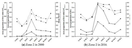
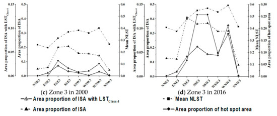
Figure 7.
Variations of mean normalized LST (NLST), area proportion of ISA, area proportion of ISA with LSTClass 4, and area proportion of hot spot area in each sector of two zones in 2000 and 2016: (a–d) urban zone 2 in 2000, urban zone 2 in 2016, urban zone 3 in 2000 and urban zone 3 in 2016, respectively.
Figure 7 shows that the change trends in area proportions for the high LST category (LSTClass 4) in the sectors were generally similar to the changes in ISA proportion in Zones 2 and 3. From 2000 to 2016, there was an increase in the area proportion with high LST (LSTClass 4) for some sectors of Zones 2 and 3, especially from sectors SSE2 to NNW2 of Zone 2 and from ESE3 to WNW3 of Zone 3. In the other sectors of Zones 2 and 3, the area proportion changed very little because urban expansion was limited by the north mountainous terrain.
In Figure 7, though mean NLST, area proportions of ISA and high LST area in some sectors were higher in Zone 2 than in Zone 3 in 2000 and 2016, urban expansion resulted in greater ISA increase in some sectors of Zone 3 than in Zone 2 (Figure 4). This can also be shown by the increase of the hotspot area between the two dates, which also increased more in some sectors of Zone 3 than the equivalent sectors in Zone 2. Similar to the change trend of the area proportion with high LST in the sectors, the increases in area proportion of the hotspot area were small in some sectors of Zone 3, because the terrain limited the urban expansion in these sectors. In these two zones, the area proportion of high LST area increased more in some sectors such as NNE2, ENE2, and NNW2 of Zone 2, than in sectors NNE3, ENE3, and NNW3 (in the same directions as in Zone 2) of Zone 3 from 2000 to 2016 because of the limitation by the mountainous terrain. The increases in area proportions of ISA were higher in directions of NNE, ESE, SSE, and NNW in Zone 3 than in Zone 2. This reflected that, though the area and area proportions of ISA increased more in some directions of Zone 3 than in Zone 2, because the urban expansion with an ISA increase is not continuous in space, the area of hotspots may not increase proportionally in some sectors. An analysis of the variation of area proportion of hotspot areas ISA and LST in different sectors can provide information on urban landscapes and their thermal environmental structure in different degrees of development and different directions of urban areas. This can help to cope with the urban thermal environmental change on human health.
In order to further analyse the degree of transformation from pervious to impervious surface and its impact on the thermal environment, proportional ranges of 0%–25%, 25%–50%, 50%–75% and 75%–100% were used to reclassify the area proportion of hotspot areas in each sector into four separate groups (Figure 8). Similarly, four levels of LST aggregation densities were defined by the threshold values as 0%–25% for low-density, 25%–50% for medium density, 50%–75% for sub-high density and 75%–100% for high-density of LST aggregation. Hotspot density shows the degree of LST aggregation within each sector.
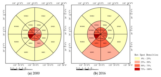
Figure 8.
Classification of the 24 sectors of three zones into four levels of LST aggregation densities on the basis of areal proportion of hot spot area at each sector in 2000 and 2016. (a) hotspot densities in 2000; (b) hotspot densities in 2016.
Figure 8 shows that the hotspot density decreased from the city centre (Zone 1) to the peripheral areas (Zone 3). High and sub-high hotspot density areas are represented in some sectors of Zone 1 and Zone 2 in both dates. However, the variations of hotspot density showed a general increase from Zone 1 to Zone 3 from 2000 to 2016. Comparing Figure 8a,b, the variations of hotspot levels indicated the degree of pervious to impervious surface transformation and its impact on the urban thermal environment. Zone 1 nearly had no landscape pattern change between the two dates. Therefore, hotspot severity levels of Zone 1 were also unvaried though LST of Zone 1 varied and even decreased in some sectors (Figure 5) between the two dates. As for the urbanization in the urban fringe, some areas in Zones 2 and 3 (especially the southern periphery of the city) was developed as a planned satellite town with large residential, commercial and industrial complexes to accommodate the increasing population. This phenomenon can be verified by the transformation of the hotspot densities of some sectors between the two dates. From 2000 to 2016, sectors WSW2, WNW2, NSW2, SSE3 and SSW3 transformed from low-density to medium-density sectors as a result of urban expansion. The low-density SSW2 and medium-density SSE2 sectors transformed to sectors of sub-high density in the same period. Since 2000, these sectors have developed as urban temperature hotspots due to the increasing construction of urban buildings and roads with a reduction of pervious surface.
4. Discussion
Hotspot analysis can provide a better understanding of the urban thermal environment by analysing the spatio-temporal patterns of LST aggregation at different dates. Because of the seasonal difference, the LST increase in some urban areas between different dates may not indicate urban expansion but seasonality. Figure 6 shows that some hotspot areas increased in some sectors of Zones 2 and 3 from 2000 to 2016, which indicates that urban expansion leading to a percent ISA increase were spatially continuous in these hotspot areas. Therefore, if ISA increases spatially continuously between the two dates, the hotspot locations increase between two dates because LST aggregation is impacted by continuous spatial changes of ISA. The urban expansion increased the number and distribution of hotspots and intensified the urban thermal environment. Spatial pattern analysis of hotspot locations can help cities to adapt effectively to climate change under conditions of urban expansion.
Urbanization brings about a variation of microclimate which impacts the comfort and physical wellbeing of the residents. The four level classifications of urban LST aggregation indicating hotspot severity represent the impact of urban expansion on the thermal environment. In this study, the spatial dynamics of hotspots from 2000 to 2016 showed that the urbanization process dominated in those sectors of the southern and western city and resulted in variations of hotspot densities in these sectors. Spatio-temporal analysis of hotspots and their sectoral distribution supports UHI mitigation and urban land use planning. The findings from the spatio-temporal analysis of hotspots and their sectoral distribution are helpful for urban planning and coping with the climatic change on human health.
This paper is a contribution to the improvement in the research on the impact of urban expansion on the thermal environment. However, the study has some limitations. The research is focused only on one city and future research needs to compare the findings with other cities. Another limitation is that the ISA change threshold needs to be further explored with a view to selecting an optimum threshold value. In addition, only bi-temporal images are selected in this study. Future studies need to compare the hotspot pattern change among different seasons to analyse the impact of seasonal variations on the distribution of hotspot patterns and how they are impacted by the distribution of impervious surfaces.
5. Conclusions
The LST hotspot locations and their change can indicate the urban expansion with transformation from pervious to impervious surface continuously in space and the variation on thermal environment. This study has provided a methodology to characterize the urban thermal environment with urban landscape pattern change instead of LST change data. The LST clustering was calculated by hotspot analysis to show the thermal intensities in different sub-divisions, and the variation of LST spatial aggregation and urban expansion between 2000 and 2016 were further analysed to generalize the pattern of urban landscape change.
By analysing the variations of mean NLST, the area proportion of ISA, the area proportion of ISA with high LST area, and the area proportion of hotspot area in each sector between the two dates, the landscape pattern change and its impact on the thermal environment were characterized in different spatial directions. Four main conclusions can be drawn from the above analysis:
(1) The sectoral hotspot division provided the directional and spatial concentration of high LST areas and further helped to delineate landscape transformation of different areas. The analytical method is helpful for urban planning and adapting to the variation of the thermal environment.
(2) Spatial dynamics of LST aggregation by sectors between the two dates showed that urbanization mainly dominated in sectors SSE2, SSW2, WSW2, WNW2, NSW2, SSE3, and SSW3, which may be treated as prioritized management areas.
(3) The analytical results show that the spatial pattern analysis of hotspots in four classes of densities can provide a good method for multi-temporal analysis on urban thermal environment, comparison of urban LST intensities and mapping the direction of urban expansion.
(4) The results showed that the hotspots areas generally increased positively with increasing ISA in the sectors between the two dates though LST change between the different dates is impacted by seasonal differences of the acquisition dates. However, in some sectors, the urban expansion with the ISA increase was not continuous in space, the hotspot area may not increase as much as the ISA increased.
This study presents an approach combining urban landscape patterns with LST aggregation analysis in different directions and development areas. Though there may be some uncertainties such as LST classification and sectors classification in the methodological framework, the findings are helpful for urban planning and coping with urban climatic change. Further studies are advised to consider aspects such as estimating the urban cooling effect of urban green spaces by analysing the location of cold spots, the thermal environmental changes along with the different seasons, and comparison of LST aggregation pattern in different cities. In addition, though Ke et al. [70] proved that, given that the same atmospheric correction methods, the NDVI derived from multiple sensors such as Landsat TM/ETM+ and OLI instruments had good consistency, further evaluation of the agreement in surface reflectance and vegetation indices derived from multiple sensors is required because of the spectral differences between these sensors.
Author Contributions
Y.Z. and X.W. collected and processed the data, performed the analysis and wrote the paper. H.B. contributed to the interpretation of the results, defined the methodology and reviewed the manuscript. B.Q. and J.C. contributed to the analysis of the data.
Funding
This research was funded by Fujian Natural Science Foundation, China (2018J01739), Fujian special funds for scientific research on public causes, China (2019R1002-2), and Key Laboratory of Spatial Data Mining & Information Sharing of Ministry of Education, Fuzhou University, Fuzhou, China (2018LSDMIS08). H. B. was supported by the UK Natural Environment Research Council (NERC) through the National Centre for Earth Observation. The work of B. Q. was supported by the National Natural Science Foundation of China (41771468, 41471362).
Acknowledgments
The authors would like to thank the three anonymous reviewers and editors, whose constructive criticism helped to improve the quality of the manuscript.
Conflicts of Interest
The authors declare no conflict of interest.
References
- Song, X.; Sexton, J.; Huang, C.; Channan, S.; Townshend, J. Characterizing the magnitude, timing and duration of urban growth from time series of Landsat-based estimates of impervious cover. Remote Sens. Environ. 2016, 175, 1–13. [Google Scholar] [CrossRef]
- Yao, R.; Wang, L.; Huang, X.; Niu, Z.; Liu, F.; Wang, Q. Temporal trends of surface urban heat islands and associated determinants in major Chinese cities. Sci. Total Environ. 2017, 609, 742–754. [Google Scholar] [CrossRef] [PubMed]
- Majumdar, D.; Biswas, A. Quantifying land surface temperature change from LISA clusters: An alternative approach to identifying urban land use transformation. Landsc. Urban Plan. 2016, 153, 51–65. [Google Scholar] [CrossRef]
- Zhang, Y.; Balzter, H.; Liu, B.; Chen, Y. Analyzing the Impacts of Urbanization and Seasonal Variation on Land Surface Temperature Based on Subpixel Fractional Covers Using Landsat Images. IEEE J. Sel. Top. Appl. Earth Obs. Remote Sens. 2017, 10, 1344–1356. [Google Scholar] [CrossRef]
- Yao, R.; Wang, L.; Huang, X.; Gong, W.; Xia, X. Greening in Rural Areas Increases the Surface Urban Heat Island Intensity. Geophys. Res. Lett. 2019, 46, 2204–2212. [Google Scholar] [CrossRef]
- Trenberth, K.; Jones, P.; Ambenje, P.; Bojariu, R.; Easterling, D.; Klein Tank, A.; Parker, D.; Rahimzadeh, F.; Renwick, J.A.; Rusticucci, M.; et al. Observations: Surface and atmospheric climate change. In Climate Change 2007: The Physical Science Basis. In Contribution of Working Group I to the Fourth Assessment Report of the Intergovernmental Panel on Climate Change; Solomon, S., Qin, D., Manning, M., Chen, Z., Marquis, M., Averyt, K.B., Tignor, M., Miller, H.L., Eds.; Cambridge University Press: Cambridge, UK; New York, NY, USA, 2007. [Google Scholar]
- Zhou, W.; Huang, G.; Cadenasso, M.L. Does spatial configuration matter? Understanding the effects of land cover pattern on land surface temperature in urban landscapes. Landsc. Urban Plan. 2011, 102, 54–63. [Google Scholar] [CrossRef]
- Yao, R.; Wang, L.; Huang, X.; Zhang, W.; Li, J.; Niu, Z. Inter annual variations in surface urban heat island intensity and associated drivers in China. J. Environ. Manag. 2018, 222, 86–94. [Google Scholar] [CrossRef]
- Voogt, J.; Oke, T. Thermal remote sensing of urban climates. Remote Sens. Environ. 2003, 86, 370–384. [Google Scholar] [CrossRef]
- Imhoff, M.; Zhang, P.; Wolfe, R.; Bounoua, L. Remote sensing of the urban heat island effect a cross biomes in the continental USA. Remote Sens. Environ. 2010, 114, 504–513. [Google Scholar] [CrossRef]
- He, C.; Gao, B.; Huang, Q.; Ma, Q.; Dou, Y. Environmental degradation in the urban areas of China: Evidence from multi-source remote sensing data. Remote Sens. Environ. 2017, 193, 65–75. [Google Scholar] [CrossRef]
- Shen, H.; Huang, L.; Zhang, L.; Wu, P.; Zeng, C. Long-term and fine-scale satellite monitoring of the urban heat island effect by the fusion of multi-temporal and multi-sensor remote sensed data: A 26-year case study of the city of Wuhan in China. Remote Sens. Environ. 2016, 172, 109–125. [Google Scholar] [CrossRef]
- Nichol, J. High-resolution surface temperature patterns related to urban morphology in a tropical city: A satellite-based study. J. Appl. Meteorol. 1996, 35, 135–146. [Google Scholar] [CrossRef]
- Streutker, D.R. A remote sensing study of urban heat island of Houston, Texas. Int. J. Remote Sens. 2002, 23, 2595–2608. [Google Scholar] [CrossRef]
- Yang, J.; Su, J.; Xia, J.; Jin, C.; Li, X.; Ge, Q. The Impact of Spatial Form of Urban Architecture on the Urban Thermal Environment: A Case Study of the Zhongshan District, Dalian, China. IEEE J. Sel. Top. Appl. Earth Obs. Remote Sens. 2018, 11, 2709–2716. [Google Scholar] [CrossRef]
- Peng, J.; Xie, P.; Liu, Y.; Ma, J. Urban thermal environment dynamics and associated landscape pattern factors: A case study in the Beijing metropolitan region. Remote Sens. Environ. 2016, 173, 145–155. [Google Scholar] [CrossRef]
- Zhou, W.; Wang, J.; Cadenasso, M. Effects of the spatial configuration of trees on urban heat mitigation: A comparative study. Remote Sens. Environ. 2017, 195, 1–12. [Google Scholar] [CrossRef]
- Huang, Q.; Huang, J.; Yang, X.; Fang, C.; Liang, Y. Quantifying the seasonal contribution of coupling urban land use types on Urban Heat Island using Land Contribution Index: A case study in Wuhan, China. Sustain. Cities Soc. 2019, 44, 666–675. [Google Scholar] [CrossRef]
- Bonafoni, S.; Keeratikasikorn, C. Land Surface Temperature and Urban Density: Multiyear Modeling and Relationship Analysis Using MODIS and Landsat Data. Remote Sens. 2018, 10, 1471. [Google Scholar] [CrossRef]
- Chen, Y.; Yu, S. Impacts of urban landscape patterns on urban thermal variations in Guangzhou, China. Int. J. Appl. Earth Obs. Geoinf. 2017, 54, 65–71. [Google Scholar] [CrossRef]
- Amiri, R.; Weng, Q.; Alimohammadi, A.; Alavipanah, S.K. Spatial–temporal dynamics of land surface temperature in relation to fractional vegetation cover and land use/cover in the Tabrizurbanarea, Iran. Remote Sens. Environ. 2009, 113, 2606–2617. [Google Scholar] [CrossRef]
- Weng, Q. Remote sensing of impervious surfaces in the urban areas: Requirements, methods, and trends. Remote Sens. Environ. 2012, 117, 34–49. [Google Scholar] [CrossRef]
- Rasul, A.; Balzter, H.; Smith, C. Spatial variation of the daytime Surface Urban Cool Island during the dry season in Erbil, Iraqi Kurdistan, from Landsat. Urban Clim. 2015, 14, 176–186. [Google Scholar] [CrossRef]
- Peng, J.; Jia, J.; Liu, Y.; Li, H.; Wu, J. Seasonal contrast of the dominant factors for spatial distribution of land surface temperature in urban areas. Remote Sens. Environ. 2018, 215, 255–267. [Google Scholar] [CrossRef]
- Xian, G.; Crane, M. Assessments of urban growth in the Tampa Bay watershed using remote sensing data. Remote Sens. Environ. 2005, 97, 203–215. [Google Scholar] [CrossRef]
- Yuan, F.; Bauer, M.E. Comparison of impervious surface area and normalized difference vegetation index as indicators of surface urban heat island effects in Landsat imagery. Remote Sens. Environ. 2007, 106, 375–386. [Google Scholar] [CrossRef]
- Arnold, C.L., Jr.; Gibbons, C.J. Impervious surface coverage: The emergence of a key environmental indicator. J. Am. Plan. Assoc. 1996, 62, 243–258. [Google Scholar] [CrossRef]
- Weng, Q.; Lu, D.; Schubring, J. Estimation of land surface temperature-vegetation abundance relationship for urban heat island studies. Remote Sens. Environ. 2004, 89, 467–483. [Google Scholar] [CrossRef]
- Weng, Q. Thermal infrared remote sensing for urban climate and environmental studies: Methods, applications, and trends. ISPRS J. Photogramm. Remote Sens. 2009, 64, 335–344. [Google Scholar] [CrossRef]
- Deng, C.; Wu, C. Examining the impacts of urban biophysical compositions on surface urban heat island: A spectral unmixing and thermal mixing approach. Remote Sens. Environ. 2013, 131, 262–274. [Google Scholar] [CrossRef]
- Heinl, M.; Hammerle, A.; Tappeiner, U.; Leitinger, G. Determinants of urban-rural land surface temperature differences -A landscape scale perspective. Landsc. Urban Plan. 2015, 134, 33–42. [Google Scholar] [CrossRef]
- Rotem-Mindali, O.; Michael, Y.; Helman, D.; Lensky, I.M. The role of local land-use on the urban heat island effect of Tel Aviv as assessed from satellite remote sensing. Appl. Geogr. 2015, 56, 145–153. [Google Scholar] [CrossRef]
- Wang, Y.; Hu, B.; Myint, S.; Feng, C.; Chow, W.; Passy, P. Patterns of land change and their potential impacts on land surface temperature change in Yangon, Myanmar. Sci. Total Environ. 2018, 643, 738–750. [Google Scholar] [CrossRef] [PubMed]
- Schneider, A. Monitoring land cover change in urban and peri-urban areas using dense time stacks of Landsat satellite data and a data mining approach. Remote Sens. Environ. 2012, 124, 689–704. [Google Scholar] [CrossRef]
- Lu, D.; Li, G.; Kuang, W.; Moran, E. Methods to extract impervious surface areas from satellite images. Int. J. Digit. Earth. 2013, 7, 93–112. [Google Scholar] [CrossRef]
- Gallo, K.P.; McNab, A.L.; Karl, T.R.; Brown, J.F.; Hood, J.J.; Tarpley, J.D. The use of a vegetation index for assessment of the urban heat island effect. Int. J. Remote Sens. 1993, 11, 2223–2230. [Google Scholar] [CrossRef]
- Gallo, K.P.; Owen, T.W. Satellite Based Adjustments for the Urban Heat Island Temperature Bias. J. Appl. Meteorol. 1999, 38, 806–813. [Google Scholar] [CrossRef]
- Zhang, X.; Zhong, T.; Feng, X.; Wang, K. Estimation of the relationship between vegetation patches and urban land surface temperature with remote sensing. Int. J. Remote Sens. 2009, 30, 2105–2118. [Google Scholar] [CrossRef]
- Zhang, Y.; Balzter, H.; Zou, C.; Xu, H.; Tang, F. Characterizing bi-temporal patterns of land surface temperature using landscape metrics based on sub-pixel classifications from Landsat TM/ETM+. Int. J. Appl. Earth Obs. Geoinf. 2015, 42, 87–96. [Google Scholar] [CrossRef]
- Oke, T.R. The energetic basis of the urban heat island. Q. J. R. Meteorol. Soc. 1982, 108, 1–24. [Google Scholar] [CrossRef]
- Zhang, Y.; Odeh, I.; Ramadan, E. Assessment of land surface temperature in relation to landscape metrics and fractional vegetation cover in an urban/peri-urban region using Landsat data. Int. J. Remote Sens. 2013, 34, 168–189. [Google Scholar] [CrossRef]
- Zhang, Y.; Harris, A.; Balzter, H. Characterizing fractional vegetation cover and land surface temperature based on sub-pixel fractional impervious surfaces from Landsat TM/ETM+. Int. J. Remote Sens. 2015, 36, 4213–4232. [Google Scholar] [CrossRef]
- Feyisa, G.; Meilby, H.; Jenerette, G.; Pauliet, S. Locally optimized separability enhancement indices for urban land cover mapping: Exploring thermal environmental consequences of rapid urbanization in Addis Ababa, Ethiopia. Remote Sens. Environ. 2016, 175, 14–31. [Google Scholar] [CrossRef]
- Berk, A.; Anderson, G.; Acharya, P.; Chetwynd, J.; Bernstein, L.; Shettle, E.; Matthew, M.; Adler-Golden, S. MODTRAN 4 User’s Manual; Air Force Research Laboratory: North Andover, MA, USA, 1999. [Google Scholar]
- Schroeder, T.; Cohen, W.; Song, C.; Canty, M.; Yang, Z. Radiometric correction of multi-temporal Landsat data for characterization of early successional forest patterns in western Oregon. Remote Sens. Environ. 2006, 103, 16–26. [Google Scholar] [CrossRef]
- Barsi, J.; Schott, J.; Palluconi, F.; Hook, S. Validation of a web-based atmospheric correction tool for single thermal band instruments. In Earth Observing Systems X; Butler, J.J., Ed.; Paper 58820E; SPIE: Bellingham, WA, USA, 2005; Volume 5882. [Google Scholar]
- Van De Grienzd, A.A.; Owe, M. On the relationship between thermal emissivity and the normalized difference vegetation index for natural surfaces. Int. J. Remote Sens. 1993, 14, 1119–1131. [Google Scholar] [CrossRef]
- Sobrino, J.A.; Raissouni, N.; Li, Z. A comparative study of land surface emissivity retrieval from NOAA data. Remote Sens. Environ. 2001, 75, 256–266. [Google Scholar] [CrossRef]
- Chander, G.; Markham, B. Revised Landsat-5 TM radiometric calibration procedures and post calibration dynamic ranges. IEEE Trans. Geosci. Remote Sens. 2003, 41, 2674–2677. [Google Scholar] [CrossRef]
- Smith, R.M. Comparing traditional methods for selecting class intervals on Choropleth maps. Prof. Geogr. 1986, 38, 62–67. [Google Scholar] [CrossRef]
- Liu, H.; Weng, Q. Seasonal variations in the relationship between landscape pattern and land surface temperature in Indianapolis, USA. Environ. Monit. Assess. 2008, 144, 199–219. [Google Scholar] [CrossRef]
- Rasul, A.; Balzter, H.; Smith, C. Applying a normalized ratio scale technique to assess influences of urban expansion on land surface temperature of the semi-arid city of Erbil. Int. J. Remote Sens. 2017, 38, 3960–3980. [Google Scholar] [CrossRef]
- Adams, J.; Sabol, D.; Kapos, V.; Filho, R.; Roberts, D.; Smith, M.; Gillespie, A. Classification of multispectral images based on fractions of endmembers: Application to land cover change in the Brazilian Amazon. Remote Sens. Environ. 1995, 52, 137–154. [Google Scholar] [CrossRef]
- Mustard, J.F.; Sunshine, J.M. Spectral analysis for earth science: Investigations using remote sensing data. In Remote Sensing for the Earth Sciences: Manual of Remote Sensing, 3rd ed.; Rencz, A.N., Ed.; John Wiley & Sons: New York, NY, USA, 1999; Volume 3. [Google Scholar]
- Mitraka, Z.; Chrysoulakis, N.; Kamarianakis, Y.; Partsinevelos, P.; Tsouchlaraki, A. Improving the estimation of urban surface emissivity based on sub-pixel classification of high resolution satellite imagery. Remote Sens. Environ. 2012, 117, 125–134. [Google Scholar] [CrossRef]
- Boardman, J.W.; Kruse, F.A.; Green, R.O. Mapping target signatures via partial unmixing of AVIRIS data. In Proceedings of the Summaries of the 5th Annual JPL Airborne Geoscience Workshop, Pasadena, CA, USA, 23–26 January 1995; Jet Propulsion Laboratory Publications: Pasadena, CA, USA, 1995. [Google Scholar]
- Yang, J.; He, Y.; Oguchi, T. An endmember optimization approach for linear spectral unmixing of fine-scale urban imagery. Int. J. Appl. Earth Obs. Geoinf. 2014, 27, 137–146. [Google Scholar] [CrossRef]
- Wu, C.; Murray, A.T. Estimating impervious surface distribution by spectral mixture analysis. Remote Sens. Environ. 2003, 84, 493–505. [Google Scholar] [CrossRef]
- Singh, A. Digital change detection techniques using remotely-sensed data. Int. J. Remote Sens. 1989, 10, 989–1003. [Google Scholar] [CrossRef]
- Sexton, J.O.; Noojipady, P.; Anand, A.; Song, X.P.; McMahon, S.; Huang, C.; Feng, M.; Channan, S.; Townshend, J.R. A model for the propagation of uncertainty from continuous estimates of tree cover to categorical forest cover and change. Remote Sens. Environ. 2015, 156, 418–425. [Google Scholar] [CrossRef]
- Carrión-Flores, C.; Irwin, E.G. Determinants of residential land-use conversion and sprawl at the rural-urban fringe. Am. J. Agric. Econ. 2004, 86, 889–904. [Google Scholar] [CrossRef]
- Seto, K.C.; Fragkias, M.; Güneralp, B.; Reilly, M.K. A meta-analysis of global urban land expansion. PLoS ONE 2011, 6, e23777. [Google Scholar] [CrossRef]
- Gao, F.; De Colstoun, E.B.; Ma, R.; Weng, Q.; Masek, J.G.; Chen, J.; Pan, Y.; Song, C. Mapping impervious surface expansion using medium-resolution satellite image time series: A case study in the Yangtze River Delta, China. Int. J. Remote Sens. 2012, 33, 7609–7628. [Google Scholar] [CrossRef]
- Taubenböck, H.; Esch, T.; Felbier, A.; Wiesner, M.; Roth, A.; Dech, S. Monitoring urbanization in mega cities from space. Remote Sens. Environ. 2012, 117, 162–176. [Google Scholar] [CrossRef]
- Mertes, C.M.; Schneider, A.; Sulla-Menashe, D.; Tatem, A.J.; Tan, B. Detecting change in urban areas at continental scales with MODIS data. Remote Sens. Environ. 2015, 158, 331–347. [Google Scholar] [CrossRef]
- Tran, D.; Filiberto, P.; Latorre-Carmona, P.; Myint, S.; Caetano, M.; Kieu, H. Characterizing the relationship between land use land cover change and land surface temperature. ISPRS J. Photogramm. Remote Sens. 2017, 124, 119–132. [Google Scholar] [CrossRef]
- ESRI. How Hot Spot Analysis (Getis-OrdGi) Works? Available online: http://proarcgis.com/en/pro-app/tool-reference/spatial-statistics/h-how-hot-spot-analysis-getis-ord-gispatial-stati.htm (accessed on 16 February 2016).
- Ord, J.K.; Getis, A. Local spatial auto correlation statistics—Distributional issues and application. Geogr. Anal. 1995, 27, 286–306. [Google Scholar] [CrossRef]
- Wulder, M.; Boots, B. Local spatial autocorrelation characteristics of remotely sensed imagery assessed with the Getis statistic. Int. J. Remote Sens. 1998, 19, 2223–2231. [Google Scholar] [CrossRef]
- Ke, Y.; Im, J.; Lee, J.; Gong, H.; Ryu, Y. Characteristics of Landsat 8 OLI-derived NDVI by comparison with multiple satellite sensors and in-situ observations. Remote Sens. Environ. 2015, 164, 298–313. [Google Scholar] [CrossRef]
© 2019 by the authors. Licensee MDPI, Basel, Switzerland. This article is an open access article distributed under the terms and conditions of the Creative Commons Attribution (CC BY) license (http://creativecommons.org/licenses/by/4.0/).