Seven-Component Model-Based Decomposition for PolSAR Data with Sophisticated Scattering Models


Abstract
:
1. Introduction
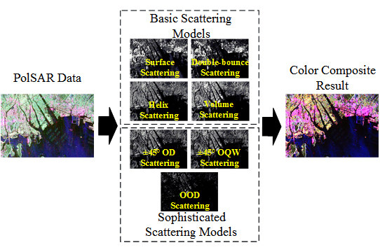
2. Methodology
2.1. Basic Scattering Model
2.2. Sophisticated Scattering Model
2.2.1. OOD Scattering Model
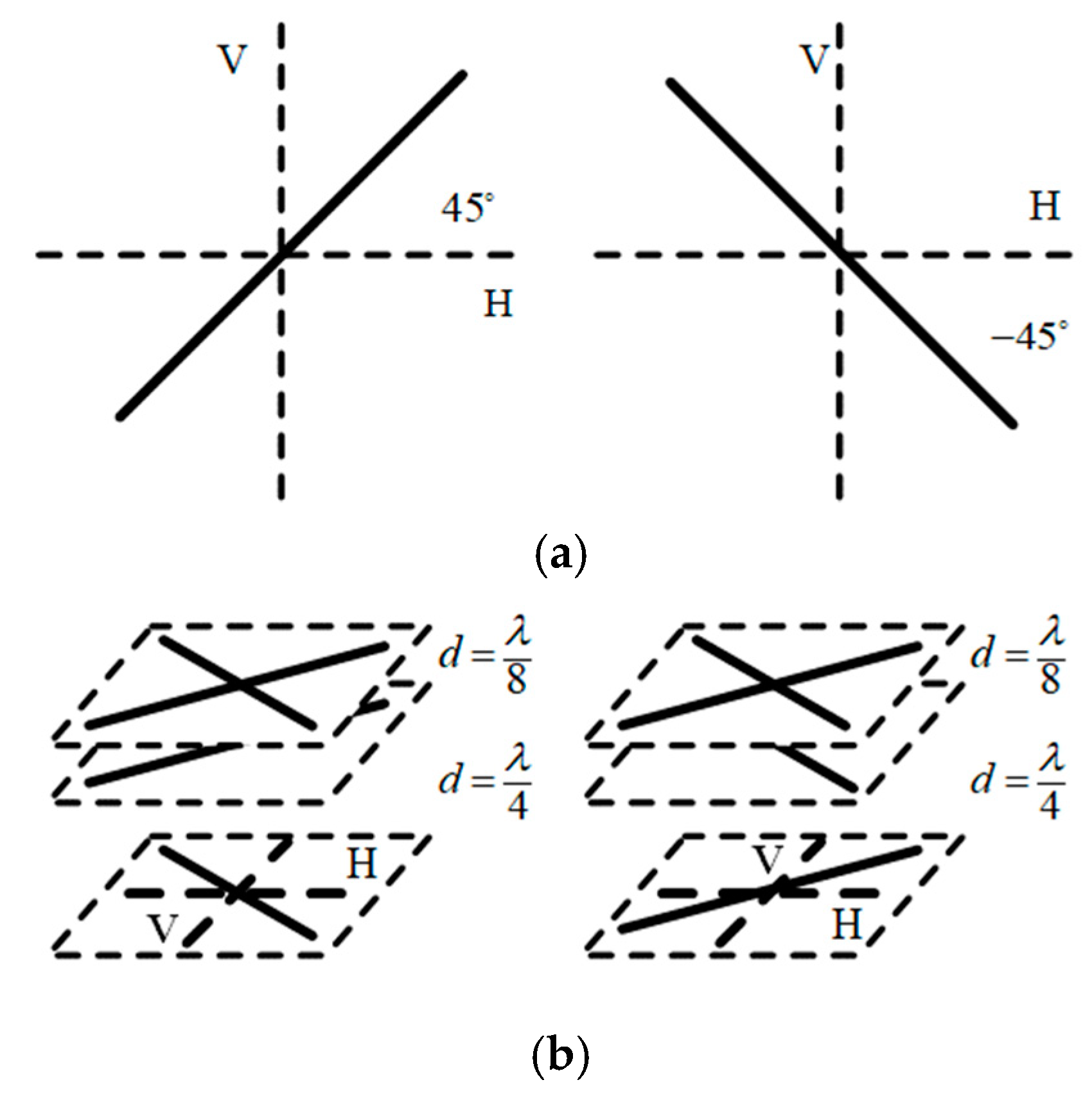
2.2.2. ±45° Oriented Dipole and Quarter-Wave Reflector Scattering Models
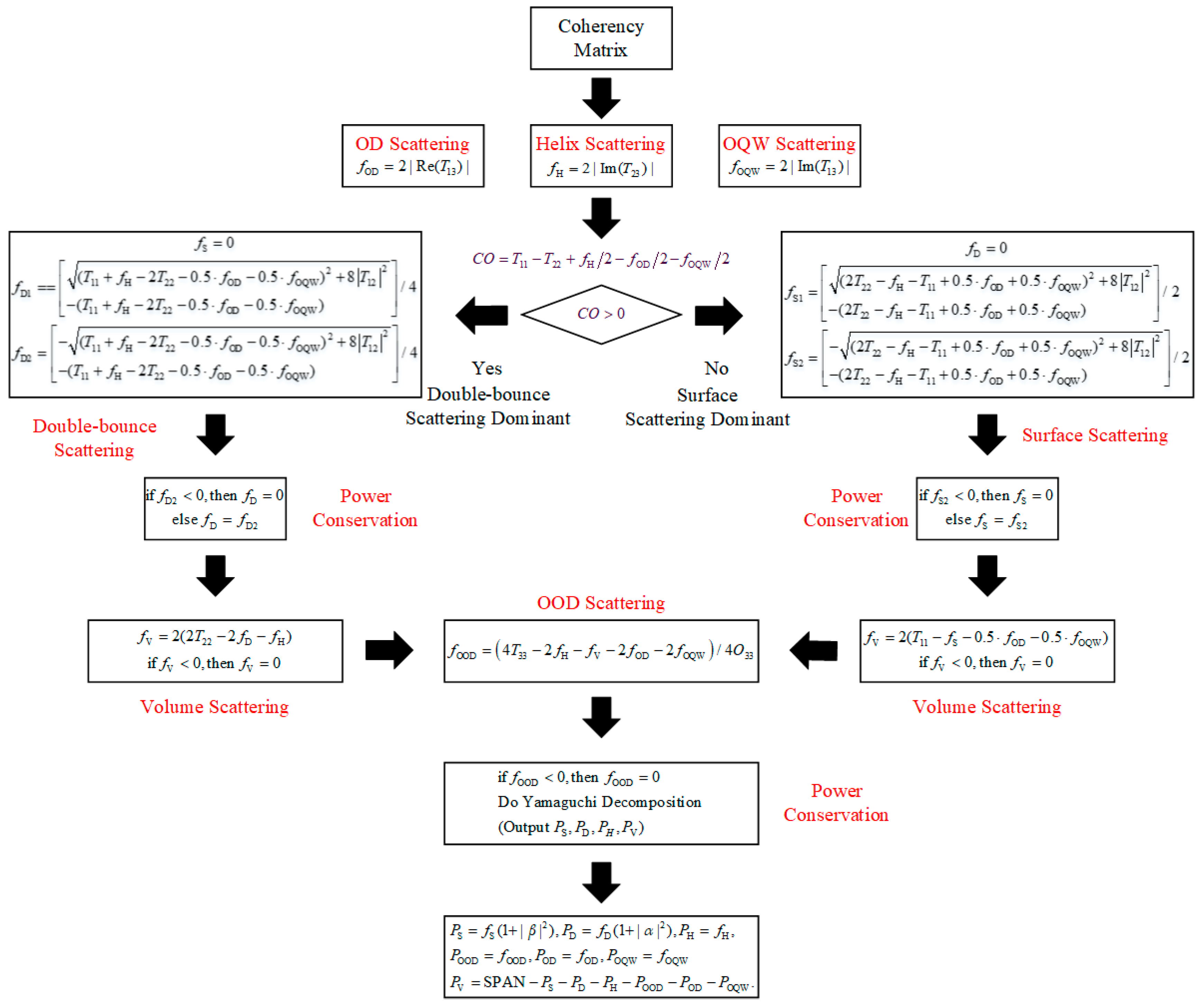
2.3. Model Solution
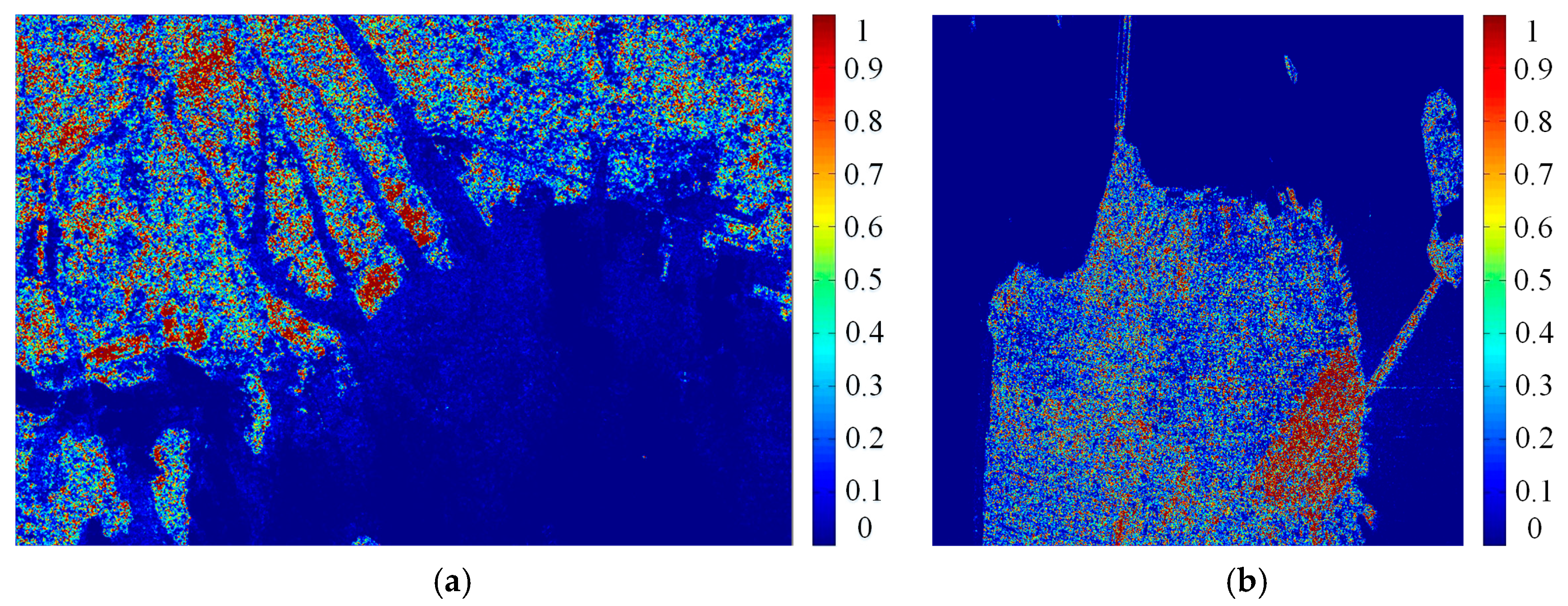
3. Experimental Results
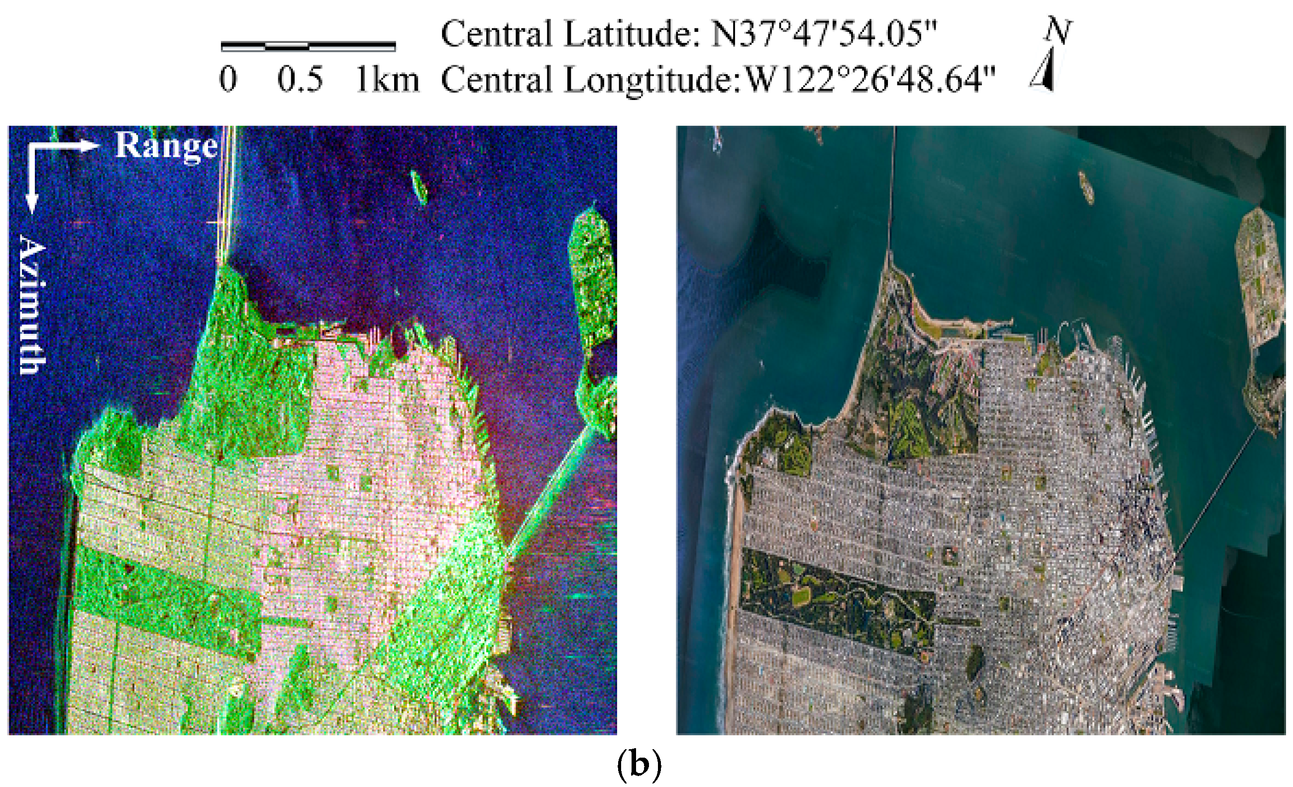
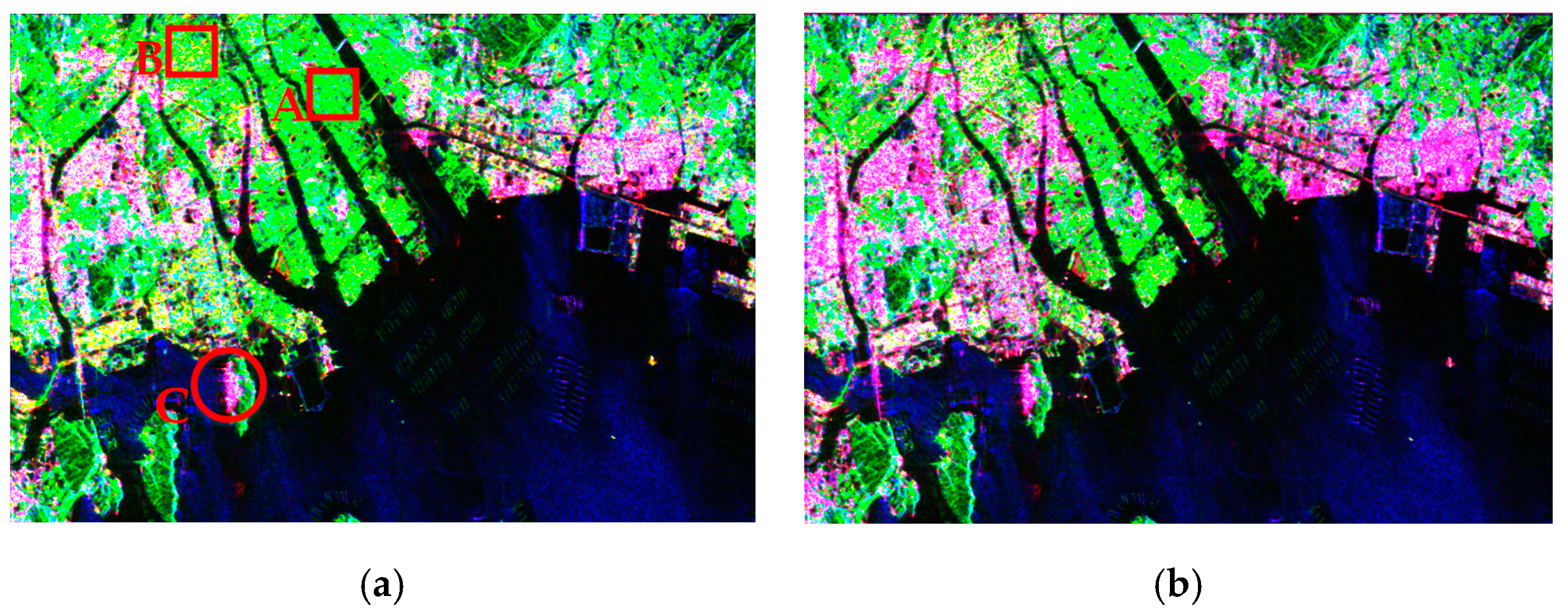
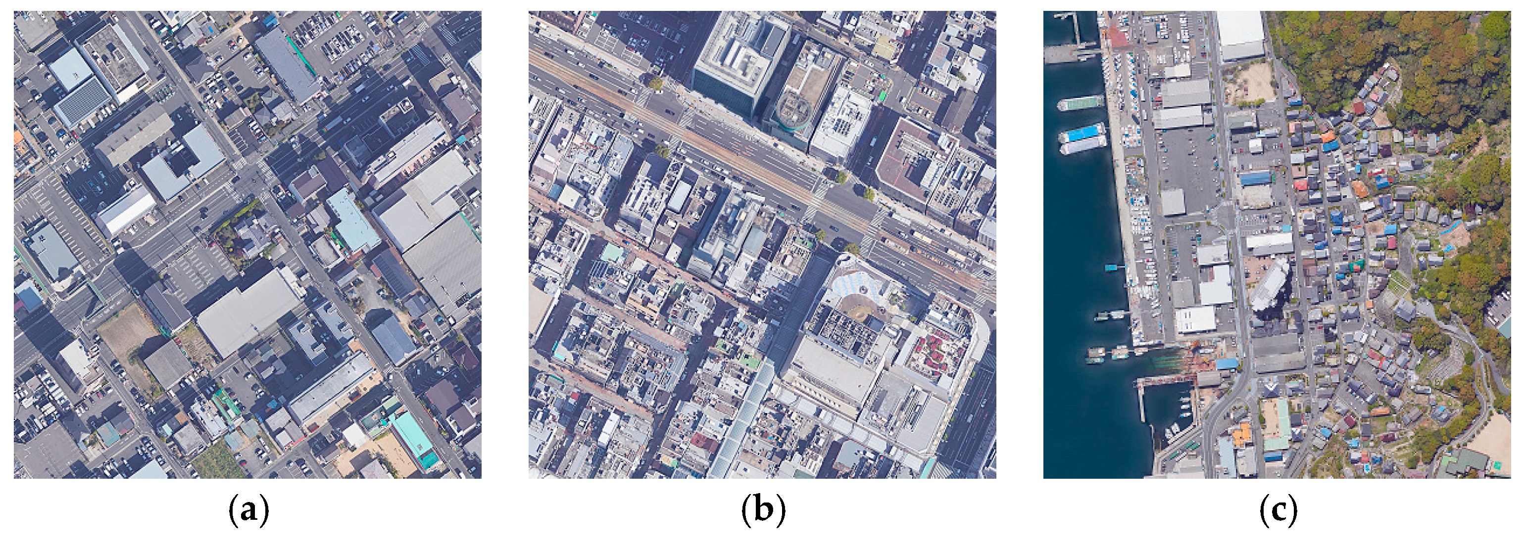
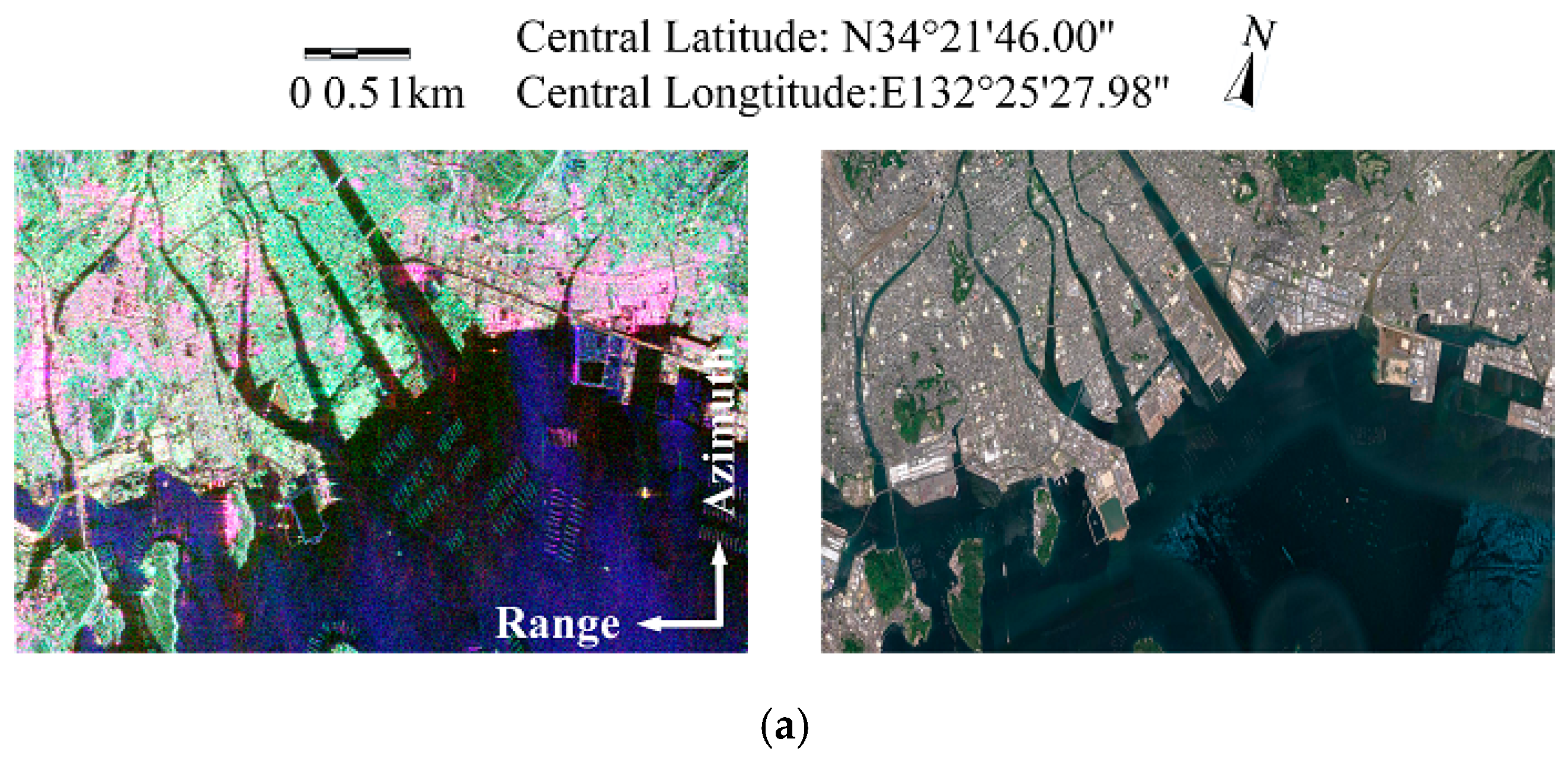
3.1. Data Description
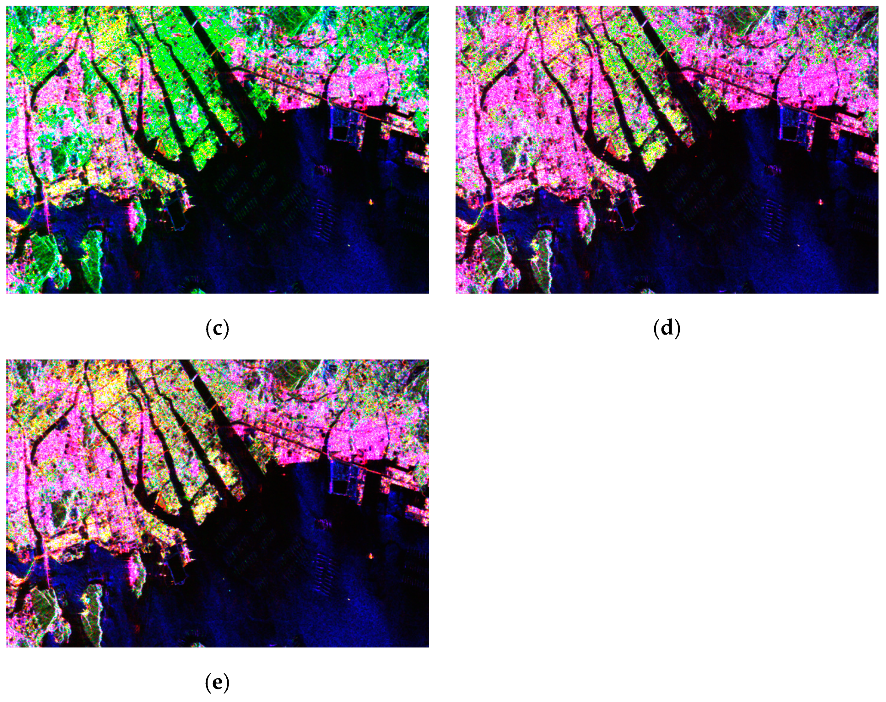
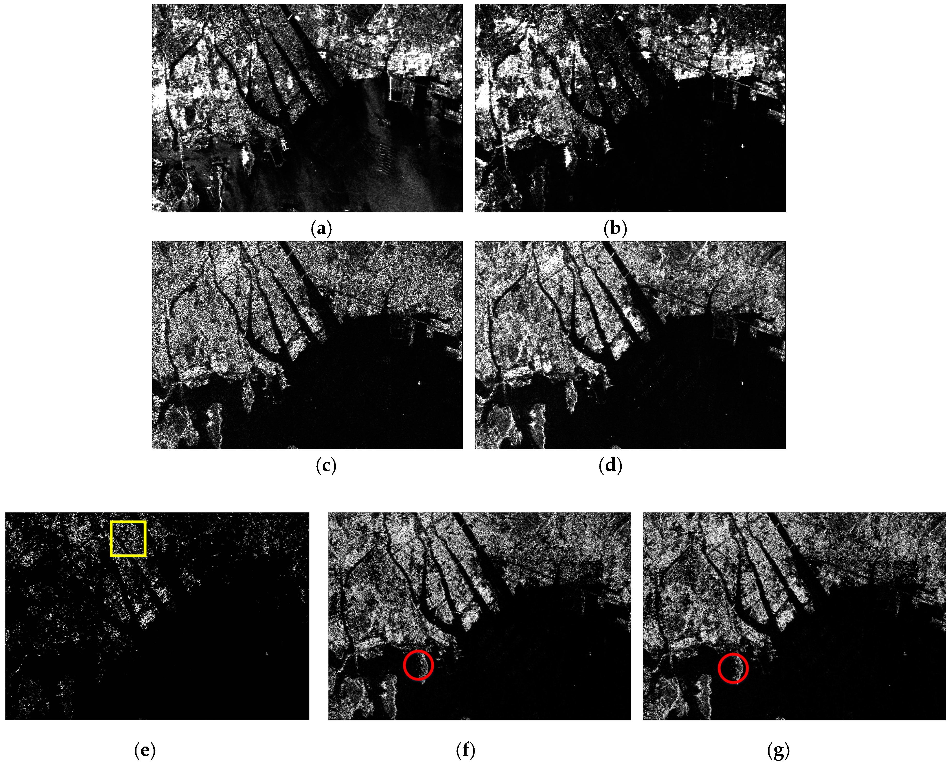
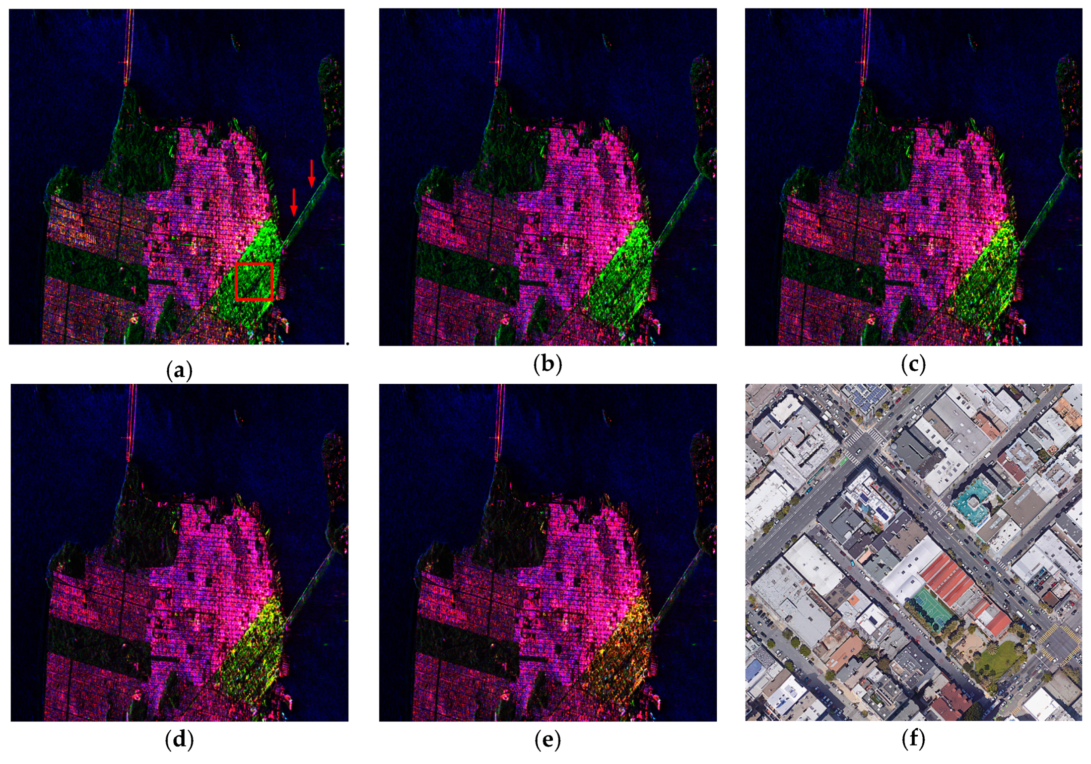
3.2. Decomposition Results on L-Band Data
3.3. Further Validation on C-Band Data
4. Discussions
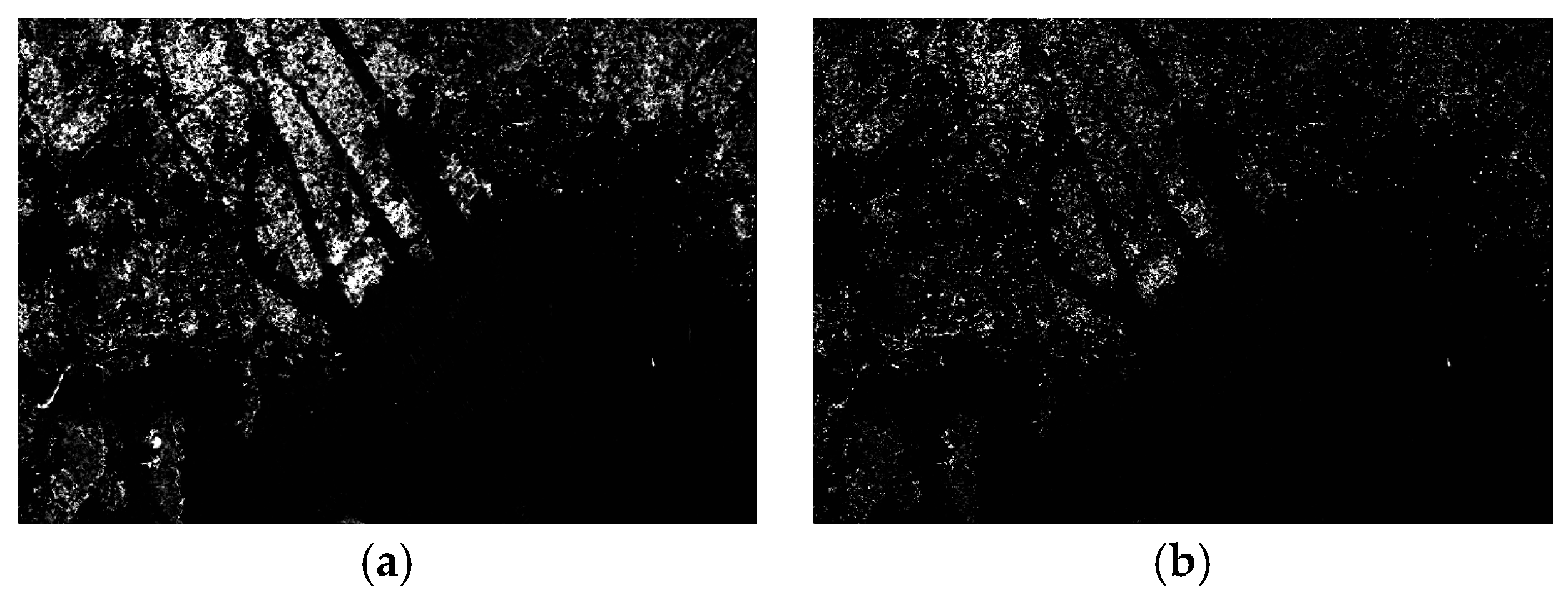
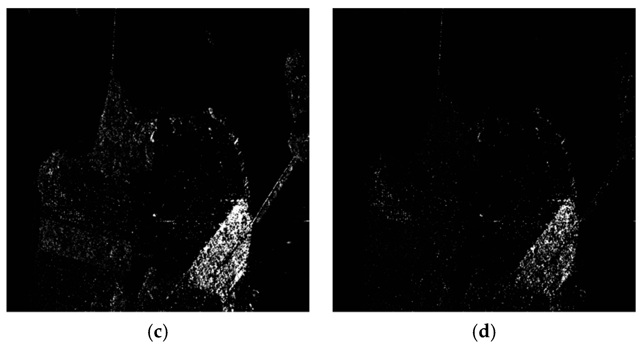
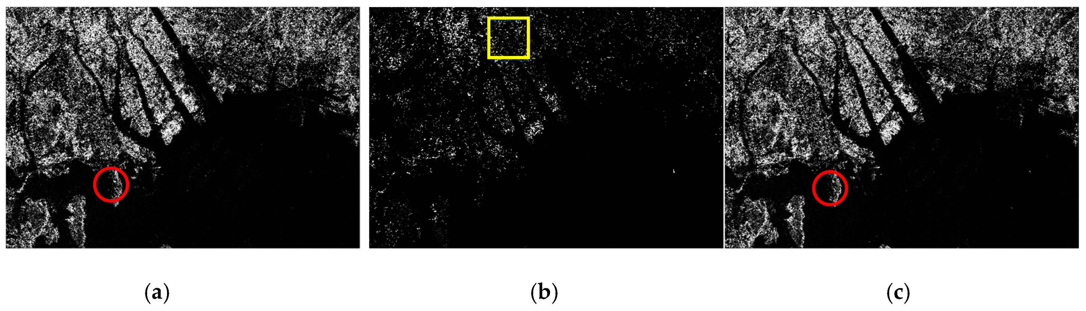
4.1. Comparison of the OOD and the Cross Scattering Models
4.2. Performance of the Modified Factor
5. Conclusions
Author Contributions
Funding
Conflicts of Interest
References
- Freeman, A.; Durden, S.L. A three-component scattering model for polarimetric SAR data. IEEE Trans. Geosci. Remote Sens. 1998, 36, 963–973. [Google Scholar] [CrossRef]
- Yamaguchi, Y.; Moriyama, T.; Ishido, M.; Yamada, H. Four-component scattering model for polarimetric SAR image decomposition. IEEE Trans. Geosci. Remote Sens. 2005, 43, 1699–1706. [Google Scholar] [CrossRef]
- Quan, S.; Xiang, D.; Xiong, B.; Hu, C.; Kuang, G. A Hierarchical Extension of General Four-Component Scattering Power Decomposition. Remote Sens. 2017, 9, 856. [Google Scholar] [CrossRef]
- Xie, Q.; Ballester-Berman, D.; Lopez-Sanchez, J.M.; Zhu, J.; Wang, C. On the use of generalized volume scattering models for the improvement of general polarimetric model-based decomposition. Remote Sens. 2017, 9, 117. [Google Scholar] [CrossRef]
- Fan, H.; Quan, S.; Dai, D.; Wang, X.; Xiao, S. Refined Model-Based and Feature-Driven Extraction of Buildings from PolSAR Images. Remote Sens. 2019, 11, 1379. [Google Scholar] [CrossRef]
- Arii, M.; van Zyl, J.J.; Kim, Y. Adaptive model-based decomposition of polarimetric SAR covariance matrices. IEEE Trans. Geosci. Remote Sens. 2010, 49, 1104–1113. [Google Scholar] [CrossRef]
- Chen, S.W.; Wang, X.S.; Li, Y.Z.; Sato, M. Adaptive model-based polarimetric decomposition using polinsar coherence. IEEE Trans. Geosci. Remote Sens. 2013, 52, 1705–1718. [Google Scholar] [CrossRef]
- Bhattacharya, A.; Singh, G.; Manickam, S.; Yamaguchi, Y. An adaptive general four-component scattering power decomposition with unitary transformation of coherency matrix (AG4U). IEEE Geosci. Remote Sens. Lett. 2015, 12, 2110–2114. [Google Scholar] [CrossRef]
- Zou, B.; Zhang, Y.; Cao, N.; Minh, N.P. A four-component decomposition model for PolSAR data using asymmetric scattering component. IEEE J. Sel. Topics Appl. Earth Observ. Remote Sens. 2015, 8, 1051–1061. [Google Scholar] [CrossRef]
- Yajima, Y.; Yamaguchi, Y.; Sato, R.; Yamada, H.; Boerner, W.M. POLSAR image analysis of wetlands using a modified four-component scattering power decomposition. IEEE Trans. Geosci. Remote Sens. 2008, 46, 1667–1673. [Google Scholar] [CrossRef]
- Krogager, E. Aspects of Polarimetric Radar Imaging. Doctoral Thesis, Technical University of Denmark, Copenhagen, Denmark, 1993. [Google Scholar]
- Van Zyl, J.J.; Arii, M.; Kim, Y. Model-based decomposition of polarimetric SAR covariance matrices constrained for nonnegative eigenvalues. IEEE Trans. Geosci. Remote Sens. 2011, 49, 3452–3459. [Google Scholar] [CrossRef]
- Cui, Y.; Yamaguchi, Y.; Yang, J.; Kobayashi, H.; Park, S.E.; Singh, G. On complete model-based decomposition of polarimetric SAR coherency matrix data. IEEE Trans. Geosci. Remote Sens. 2013, 52, 1991–2001. [Google Scholar] [CrossRef]
- Lim, Y.X.; Burgin, M.S.; van Zyl, J.J. An optimal nonnegative eigenvalue decomposition for the Freeman and Durden three-component scattering model. IEEE Trans. Geosci. Remote Sens. 2017, 55, 2167–2176. [Google Scholar] [CrossRef]
- Lee, J.S.; Ainsworth, T.L. The effect of orientation angle compensation on coherency matrix and polarimetric target decompositions. IEEE Trans. Geosci. Remote Sens. 2011, 49, 53–64. [Google Scholar] [CrossRef]
- Chen, S.W.; Wang, X.S.; Xiao, S.P.; Sato, M. General polarimetric model-based decomposition for coherency matrix. IEEE Trans. Geosci. Remote Sens. 2013, 52, 1843–1855. [Google Scholar] [CrossRef]
- Maurya, H.; Panigrahi, R.K. Polsar coherency matrix optimization through selective unitary rotations for model-based decomposition scheme. IEEE Geosci. Remote Sens. Lett. 2018, 16, 658–662. [Google Scholar] [CrossRef]
- An, W.; Xie, C.; Yuan, X.; Cui, Y.; Yang, J. Four-component decomposition of polarimetric SAR images with deorientation. IEEE Geosci. Remote Sens. Lett. 2011, 8, 1090–1094. [Google Scholar] [CrossRef]
- Singh, G.; Yamaguchi, Y.; Park, S.E. General four-component scattering power decomposition with unitary transformation of coherency matrix. IEEE Trans. Geosci. Remote Sens. 2012, 51, 3014–3022. [Google Scholar] [CrossRef]
- Sato, A.; Yamaguchi, Y.; Singh, G.; Park, S.E. Four-component scattering power decomposition with extended volume scattering model. IEEE Geosci. Remote Sens. Lett. 2011, 9, 166–170. [Google Scholar] [CrossRef]
- Zhang, L.; Zou, B.; Cai, H.; Zhang, Y. Multiple-component scattering model for polarimetric SAR image decomposition. IEEE Geosci. Remote Sens. Lett. 2008, 5, 603–607. [Google Scholar] [CrossRef]
- Xiang, D.; Ban, Y.; Su, Y. Model-based decomposition with cross scattering for polarimetric SAR urban areas. IEEE Geosci. Remote Sens. Lett. 2015, 12, 2496–2500. [Google Scholar] [CrossRef]
- Singh, G.; Yamaguchi, Y. Model-based six-component scattering matrix power decomposition. IEEE Trans. Geosci. Remote Sens. 2018, 56, 5687–5704. [Google Scholar] [CrossRef]
- Atwood, D.K.; Thirion-Lefevre, L. Polarimetric phase and implications for urban classification. IEEE Trans. Geosci. Remote Sens. 2018, 1–12. [Google Scholar] [CrossRef]
- Quan, S.; Xiang, D.; Xiong, B.; Kuang, G. Derivation of the Orientation Parameters in Built-up Areas: With Application to Model-based Decomposition. IEEE Trans. Geosci. Remote Sens. 2018, 56, 4714–4730. [Google Scholar] [CrossRef]
- Xiang, D.; Tang, T.; Ban, Y.; Su, Y.; Kuang, G. Unsupervised polarimetric SAR urban area classificationbased on model-based decomposition with cross scattering. ISPRS J. Photogramm. RemoteSens. 2016, 116, 86–100. [Google Scholar] [CrossRef]
- Hong, S.H.; Wdowinski, S. Double-bounce component in cross-polarimetric SAR from a new scattering target decomposition. IEEE Trans. Geosci. Remote Sens. 2013, 52, 3039–3051. [Google Scholar] [CrossRef]
- Li, H.; Li, Q.; Wu, G.; Chen, J.; Liang, S. The impacts of buildings orientation on polarimetric orientation angle estimation and model-based decomposition for multilook polarimetric SAR data in urban areas. IEEE Trans. Geosci. Remote Sens. 2016, 54, 5520–5532. [Google Scholar] [CrossRef]
- Quan, S.; Xiong, B.; Xiang, D.; Hu, C.; Kuang, G. Scattering characterization of obliquely oriented buildingss from PolSAR data using eigenvalue-related model. Remote Sens. 2019, 11, 581. [Google Scholar] [CrossRef]
- Quan, S.; Xiong, B.; Xiang, D.; Zhao, L.; Zhang, S.; Kuang, G. Eigenvalue-based urban area extraction using polarimetric SAR data. IEEE J. Sel. Topics Appl. Earth Observ. Remote Sens. 2018, 11, 458–471. [Google Scholar] [CrossRef]
- Lee, J.S.; Pottier, E. Polarimetric Radar Imaging: From Basics to Applications; Taylor Francis: Boca Raton, FL, USA, 2009; pp. 85–158. ISBN 9781420054972. [Google Scholar]
- Cloude, S.R. Polarisation: Applications in Remote Sensing; Oxford University Press: New York, NY, USA, 2010; pp. 57–65. ISBN 9780191574382. [Google Scholar]
- Chen, S.W.; Ohki, M.; Shimada, M.; Sato, M. Deorientation effect investigation for model-based decomposition over oriented built-up areas. IEEE Geosci. Remote Sens. Lett. 2013, 10, 273–277. [Google Scholar] [CrossRef]


| Proposed | S6D | 5SD | S4R | Y4D | |
|---|---|---|---|---|---|
| Surface scattering | 25.59% | 24.54% | 14.77% | 13.48% | 12.85% |
| Double-bounce scattering | 6.87% | 9.10% | 5.00% | 5.67% | 2.19% |
| Volume scattering | 38.51% | 50.62% | 71.03% | 74.31% | 78.41% |
| Helix scattering | 6.55% | 6.55% | 6.55% | 6.55% | 6.55% |
| OOD/Cross scattering | 4.68% | —— | 2.65% | —— | —— |
| ±45° OD scattering | 9.45% | 9.43% | —— | —— | —— |
| ±45° OQW scattering | 8.73% | 8.57% | —— | —— | —— |
| Urban scattering | 36.28% | 33.65% | 14.2% | 12.22% | 8.74% |
| Proposed | S6D | 5SD | S4R | Y4D | |
|---|---|---|---|---|---|
| Surface scattering | 18.95% | 16.26% | 17.59% | 16.93% | 9.34% |
| Double-bounce scattering | 17.39% | 20.34% | 15.99% | 17.50% | 6.06% |
| Volume scattering | 32.03% | 36.24% | 54.99% | 58.40% | 77.43% |
| Helix scattering | 7.17% | 7.17% | 7.17% | 7.17% | 7.17% |
| OOD/Cross scattering | 5.18% | —— | 4.27% | —— | —— |
| ±45° OD scattering | 11.63% | 12.51% | —— | —— | —— |
| ±45° OQW scattering | 7.65% | 7.48% | —— | —— | —— |
| Urban scattering | 49.02% | 47.5% | 27.43% | 24.67% | 13.23% |
| Proposed | S6D | 5SD | S4R | Y4D | |
|---|---|---|---|---|---|
| Surface scattering | 12.29% | 6.50% | 4.55% | 4.55% | 3.45% |
| Double-bounce scattering | 14.84% | 6.49% | 3.53% | 5.21% | 0.83% |
| Volume scattering | 24.23% | 48.68% | 59.21% | 77.59% | 83.09% |
| Helix scattering | 12.63% | 12.63% | 12.63% | 12.63% | 12.63% |
| OOD/Cross scattering | 13.79% | —— | 20.08% | —— | —— |
| ±45° OD scattering | 12.50% | 14.72% | —— | —— | —— |
| ±45° OQW scattering | 9.72% | 10.98% | —— | —— | —— |
| Urban scattering | 63.48% | 44.82% | 36.24% | 17.84% | 13.46% |
| Coherency Matrix Element | ||||||
|---|---|---|---|---|---|---|
| Value | 0.3558 | 0.1280 | 0.3317 | 0.0152 | −0.0368 | −0.0965 |
| −0.0104i | −0.0713i | −0.0513i | ||||
| Actual Proportion (/) | 2.59 | |||||
| Scattering Model | Proportion (/) | ||
|---|---|---|---|
| Cross Scattering Model | 0.5242 | 0.4758 | 0.91 |
| OOD Scattering Model | 0.3116 | 0.6884 | 2.21 |
© 2019 by the authors. Licensee MDPI, Basel, Switzerland. This article is an open access article distributed under the terms and conditions of the Creative Commons Attribution (CC BY) license (http://creativecommons.org/licenses/by/4.0/).
Share and Cite
Fan, H.; Quan, S.; Dai, D.; Wang, X.; Xiao, S. Seven-Component Model-Based Decomposition for PolSAR Data with Sophisticated Scattering Models. Remote Sens. 2019, 11, 2802. https://doi.org/10.3390/rs11232802
Fan H, Quan S, Dai D, Wang X, Xiao S. Seven-Component Model-Based Decomposition for PolSAR Data with Sophisticated Scattering Models. Remote Sensing. 2019; 11(23):2802. https://doi.org/10.3390/rs11232802
Chicago/Turabian StyleFan, Hui, Sinong Quan, Dahai Dai, Xuesong Wang, and Shunping Xiao. 2019. "Seven-Component Model-Based Decomposition for PolSAR Data with Sophisticated Scattering Models" Remote Sensing 11, no. 23: 2802. https://doi.org/10.3390/rs11232802
APA StyleFan, H., Quan, S., Dai, D., Wang, X., & Xiao, S. (2019). Seven-Component Model-Based Decomposition for PolSAR Data with Sophisticated Scattering Models. Remote Sensing, 11(23), 2802. https://doi.org/10.3390/rs11232802