Comparing Johnson’s S_B and Weibull Functions to Model the Diameter Distribution of Forest Plantations through ALS Data

Abstract

The analysis of the diameter distribution is important for forest management since the knowledge of tree density and growing stock by diameter classes is essential to define management plans and to support operational decisions. The modeling of diameter distributions from airborne laser scanning (ALS) data has been performed through the two-parameter Weibull probability density function (PDF), but the more flexible PDF Johnson’s S_B has never been tested for this purpose until now. This study evaluated the performance of the Johnson’s S_B to predict the diameter distributions based on ALS data from two of the most common forest plantations in the northwest of the Iberian Peninsula (Eucalyptus globulus Labill. and Pinus radiata D. Don). The Weibull PDF was taken as a benchmark for the diameter distributions prediction and both PDFs were fitted with ALS data. The results show that the S_B presented a comparable performance to the Weibull for both forest types. The S_B presented a slightly better performance for the E. globulus, while the Weibull PDF had a small advantage when applied to the P. radiata data. The Johnson’s S_B PDF is more flexible but also more sensitive to possible errors arising from the higher number of stand variables needed for the estimation of the PDF parameters.

1. Introduction

Forest inventory is essential in forest management by providing information to diagnose the stands, which supports decision-makers. The inventories are traditionally based on sampling of field plots, in which tree measures are collected in a time consuming and laborious process. However, the forest mensuration has faced a new paradigm with the improvement of light detection and ranging (LiDAR) tools, especially with airborne laser scanning (ALS), which has the ability to quickly record high-accuracy 3D-data in large areas [1].

One of the most common approaches to performing an ALS forest inventory is the area-based approach (ABA), where metrics are extracted from the normalized height of the LiDAR data cloud (NHD) and used to predict the forest variables [2,3]. The growing stock assessment is the most frequent target of the inventories, but effective forest management often requires information of the timber volume distributed through the diameter at the breast height (dbh, 1.30 m) classes [4] (pp. 261–298). In this case, even though the ABA does not allow detecting tree diameters directly, it enables obtaining the forest stand structure indirectly by using the NHD metrics to estimate probability density functions (PDF) that describe diameter distributions [5].

Earlier studies [6,7] succeeded in incorporating NHD metrics to obtain the diameter distribution of boreal forests using the two-parameter Weibull distribution, especially when applying the parameter recovery approach. Other similar applications of this approach were also used by other researchers [8,9,10]. Non-parametric techniques, such as k-nearest neighbors [11] or percentiles [12], have also been applied to capture the irregularities in the diameter distribution [13,14,15,16,17,18]. Despite improving the accuracy, those methods usually do not follow biological principles and are focused on reducing the prediction errors so the interpretation of their results is not straightforward.

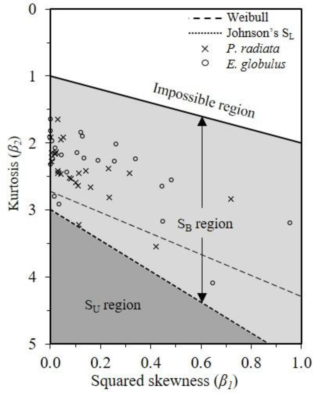
As suggested by Gobakken and Næsset [6], Johnson’s S_B distribution [19] could be tested to ALS data as an alternative to the Weibull distribution. The S_B is recognized by the scientific community as a highly flexible distribution, since it allows the representation of a large region over the plane of the β₁ and β₂ coefficients, being β₁ the squared skewness and β₂ the kurtosis [20]. This distribution has shown remarkable results when fitted using field data [21,22,23,24,25,26,27,28,29,30]. Mateus and Tomé [31] also conducted a large-scale study in Portugal and demonstrated through a skewness–kurtosis analysis that the S_B PDF is the most suitable to represent the diametric distribution of Eucalyptus globulus Labill. stands. However, to the best of our knowledge, there are no records of its applications to ALS data.

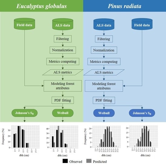
In this context, this study evaluated the ability of the S_B PDF to predict the diameter distribution of forest plantations through ALS data. The hypothesis is that the Johnson’s S_B, due to its flexibility, is more efficient than the Weibull distribution. Two datasets from pure even-aged plantations of Eucalyptus globulus Labill. and Pinus radiata D. Don. were used to support this study.

2. Materials and Methodology

2.1. Study Areas

The eucalyptus dataset was collected from a 9-km² forest area located in northwest Portugal, close to the city of Águeda (Figure 1, left). The area presented variability in its topography, with altitude varying from 70 to 220 m and slope of 2.5–34.2%. Pure even-aged eucalyptus plantations felled every 10–12 years during three rotations were dominant at the landscape, where high forest and coppice forest coexisted in the area. Many stands were multi-layered, with eucalyptus in the upper layer and dense understory occupying the lower layer (see [32,33] for more details).

The pine dataset was collected over a large area of 9.856 km², which represents the main distribution area of P. radiata in the province of Lugo (Figure 1, right), located in the Galicia region (northwest Spain). The altitude of most sites ranges 400–750 m and the slopes often exceed 15%. The forests are representative of P. radiata stands in NW of the Iberian Peninsula and are thus mainly characterized by high planting-density, low-intensity silvicultural treatments, and the presence of moderate shrub fuel loads (for more details see [34,35]).

2.2. Forest Inventory

The inventory in eucalyptus plantations was carried out between 10 June and 3 July 2008, using 45 circular plots of 400 m² that were selected based on systematic sampling, where each plot’s center was recorded using a total station and a differential Global Navigation Satellite System (GNSS). All plots covering two different stands or crossed by roads were discarded (20 plots). A total of 25 eucalyptus plots were therefore used in this study (Figure 1, left). All of them were representative of the area regarding the stand composition, structure, and rotation. Field measurements followed the Portuguese National Forest Inventory Field Manual [36]. The dbh was measured for each tree higher than 2 m. In the center of each plot, a 200-m² sub-plot was used to measure the heights of all trees higher than 2 m. The missing tree heights of the 400 m² plots were estimated using the Prodan’s model [37] fitted using the data from their respective subplots.

Table 1. Biometrical descriptions of the field data with their minimum, mean, maximum, and standard deviation (s) values.

Dataset	Variable *	Unit	Minimum	Mean	Maximum	s
Eucalyptus	dmin	cm	1.0	2.7	5.0	0.9
	$\overline{d}$	cm	4.8	8.8	13.0	2.3
	dmax	cm	10.0	17.5	23.9	4.3
	$d_g$	cm	5.5	9.6	14.0	2.5
	G	m2 ha−1	3.9	10.9	21.3	5.2
	N	stems ha−1	875	1454	2343	361
Pine	dmin	cm	3.2	8.9	22.8	5.6
	$\overline{d}$	cm	13.5	22.2	38.2	7.6
	dmax	cm	25.3	37.9	59.0	10.2
	$d_g$	cm	14.4	23.3	39.1	7.7
	G	m2 ha−1	16.7	36.9	68.1	11.0
	N	stems ha−1	393	1009	1820	425

* d_min, minimum dbh; $\overline{d}$, mean dbh; d_max, maximum dbh; d_g, quadratic mean dbh; G, basal area; N, number of trees per hectare.

presents the summary statistics for the data. More information about the eucalyptus dataset can be found in [33,38].

The pine field dataset was obtained during the winter of 2009–2010 from two different sources. The first source comprises a network of 10 permanent rectangular plots (600–1000 m² area, depending on stand density). The inventory design was focused on obtaining an adequate representation of the existing range of ages, stem densities, and site indices (for details, see [39]). The second source comprises 15 rectangular plots (1000 m² area) established for assessing the influence of thinning on crown fire potential. The inventory was designed to represent young and highly stocked stands, as these are usually fire-prone (see [40] for details). For all 25 inventory plots (Figure 1, right), dbh and total tree heights were measured in every tree. In addition, the coordinates of the four corners of each plot were obtained from topographic surveys by using a total station and a differential GNSS.

The individual tree volumes were predicted using allometric equations and summed up to obtain the ground reference value for the plot growing stocks (m³ ha⁻¹). The equations were provided by Tomé et al. [41] for the eucalyptus dataset and by Diéguez-Aranda et al. [42] for the pine dataset.

All datasets present similar behavior regarding the β₁ and β₂ coefficients computed for the tree dbh within plots (Figure 2). They are mostly spread over the area of the S_B domain, and not over the line of the Weibull distribution. This fact corroborates the higher expectation for S_B over Weibull to obtain diameter distributions for these two species.

2.3. ALS Data Acquisition and Processing

2.3.1. Eucalyptus Data

The LiDAR data covering the E. globulus plots were acquired on 14 July 2008, few days after the forest inventory, using a LiteMapper-5600 laser system with the full-waveform hardware RIEGL LMS-Q560. The airplane flew 600 m from the ground at 46.26 m s⁻¹. The parameters of the laser system were 0.5 mrad of beam divergence, ±45° of scan angle, and pulse rate of 150 kHz. The resulted swath was 497 m (60% of overlap) and the point density was 9.5 points m⁻². The ALS point clouds were processed using the FUSION software [43]. The ground points were filtered [44] and used to derive a 0.5-m-pixel digital terrain model (DTM) by triangulation. Ground reference measures collected with a differential GNNS were used to assess the vertical accuracy of the DTM (see [33]). The vertical accuracy of the ALS data, given by the root mean squared error (RMSE), was equal to 0.25 m. The DTM was applied to normalize the height data cloud, a process where the points are re-scaled to aboveground elevation. The metrics were computed for each plot considering the points higher than 1 m from the ground. The used metrics are described in

Table 2. Description of the normalized height data cloud (NHD) metrics.

Metric	Dataset		Description
	Eucal.	Pine
Hmin, Hmean, Hmax	✔	✔	Minimum, mean, and maximum height.
Hmode, Hsd, Hvar, Hcv	✔	✔	Mode, standard deviation, variance height and height’s coefficient of variation.
Hiq	✔	✔	Height interquartile amplitude
Hsqew, Hkurt	✔	✔	Height skewness and kurtosis.
Haad	✔	✔	Height average absolute deviation.
Hmad.med, Hmad.mode	✔	✔	Median of the absolute deviations from the overall height median (Hmad.med) and mode (Hmad.mode).
HL1, HL2, HL3, HL4	✔	✔	Height L moments [45].
HLskew, HLkurt, HLcv	✔	✔	Linear combinations of height L moments (skewness, kurtosis and coefficient of variation).
h01, h05, h10, h20, h25, h30, h40, h50, h60, h70, h75, h80, h90, h95, h99	✔	✔	Height percentile at 1%, 5%, ..., 99%
Cnp.Ratio	✔	✔	Canopy ratio: (Hmean − Hmin)/(Hmax − Hmin).
MeanQuad, MeanCub	✔	✖	Squared and cubic mean.
PercFAT, PercAAT	✔	✔	Percentage of first and all return above the threshold.
PercFAMean, PercAAMode	✔	✔	Percentage of first return above mean and mode.
RatioAAmeanF	✔	✔	Ratio between the first return above mean height and the number of first returns.
RatioAAmodeF	✔	✔	Ratio between the first return above mode height and the number of first returns.
S20, S40, S60, S80, S100	✔	✖	Sx is the percentage of points in x layer (e.g., S40 is the percentage of points within 20–40% of Hmax).

.

2.3.2. Pine Data

The LiDAR data covering the P. radiata plots was acquired in a nationwide survey for the PNOA (Plan Nacional de Ortofotografía de España) project between 5 September and 29 October 2009, under the direction of the Spanish Ministerio de Fomento (Dirección General del Instituto Geográfico Nacional (IGN) and Centro Nacional de Información Geográfica–CNIG), using a RIEGL LMS-Q680 sensor operated at 1064 nm. The airplane’s average flying height was 1300 m from the ground. The parameters of the laser system were: ±30° of scan angle and pulse rate of 70 kHz. A maximum of 4 returns per pulse was registered, reaching an average point density of 0.47 points m⁻². The ALS point clouds were also processed with the FUSION software [43]. The filtered ground points were triangulated to derive a 2 m-pixel DTM, which was used to normalize the point cloud. As reported by the provider (https://pnoa.ign.es/), the vertical accuracy of the ALS data, given by the RMSE, is ≤0.20 m. The set of metrics from the points laid above 1.5 m was extracted for each plot (Table 2).

2.4. Fitting of the Distributions

The Johnson’s S_B PDF (Equation (1)) originally has four parameters: λ is the scale parameter, responsible for the distribution extension; ε is the location parameter (lower limit); and γ and δ are the shape parameters. Because we are dealing with sampling, a low value for the location parameter is preferable [20,22,46], although the maximum likelihood estimation for this parameter is typically zero or close to zero [28]. For this reason, we set the location parameter to zero (ε = 0).

$$f\left(x\right)=\frac{\delta \lambda }{\sqrt{2\pi }\left(x-\mathsf{\epsilon }\right)\left(\mathsf{\epsilon }+\lambda -x\right)}exp\left\{-\frac{1}{2}{\left[\gamma +\delta \ln \left(\frac{x-\mathsf{\epsilon }}{\mathsf{\epsilon }+\lambda -x}\right)\right]}^2\right\}$$

(1)

$$\mathsf{\epsilon }<x<\mathsf{\epsilon }+\lambda ,\delta >0,-\infty <\gamma <\infty ,\lambda >0,\mathrm{and}\mathsf{\epsilon }\ge 0;f\left(x\right)=0,\mathrm{otherwise}.$$

The adaptation of three approaches were tested to fit this model: (i) the method of moments of Scolforo et al. [47] (

Table 3. Johnson’s S_B fitting based on methods of moments and percentile.

Method	ε	λ	δ	γ	Inputs
SB-Moments	0	dmax	$\frac{\mu \left(1-\mu \right)}{Sd\left(x\right)}+\frac{Sd\left(x\right)}{4}\left[\frac{1}{\mu \left(1-\mu \right)}-8\right]$	$\delta \ast ln\left(\frac{1-\mu }{\mu }\right)+\left(\frac{0.5-\mu }{\delta }\right)$	dmax, ds, $\overline{d}$
SB-Percentile	0	dmax	$\frac{Z_{95\%}}{ln\left(\frac{d_{95\%}-\epsilon }{\epsilon +\lambda -d_{95\%}}\right)-ln\left(\frac{d_{50\%}-\epsilon }{\epsilon +\lambda -d_{50\%}}\right)}$	$-\delta \ast ln\left(\frac{d_{50\%}-\epsilon }{\epsilon +\lambda -d_{50\%}}\right)$	dmax, d95%, d50%

d_max, maximum dbh; $\overline{d}$, mean dbh; $\mu =\frac{\overline{d}-\epsilon }{\lambda }$; d_s, dbh standard deviation; $Sd\left(x\right)$ = $\frac{d_{\mathrm{s}}}{\lambda }$; $Z_{95\%}$, 95% quantile of the standard normal distribution (1.6448); $d_{95\%}$, 95% percentile dbh; $d_{50\%}$, 50% percentile dbh (or median dbh).

); (ii) the percentile method of Knoebel and Burkhart [48] (Table 3); and (iii) the three-parameter recovery of Parresol [28], described below. These approaches are referred hereafter respectively as “S_B-Moments”, “S_B-Percentile”, and “S_B-3PR”. Other parameter estimation approaches were also considered but previous tests with our dataset showed a poor correlation among the parameters and NHD metrics for our dataset.

The S_B-3PR was performed according to the algorithm of Parresol et al. [49] but adapted in this work to R environment [50] using the minpack.lm package [51]. This approach estimates the parameters by solving a system of nonlinear equation using Levenberg–Marquardt optimization. In summary, the 3PR considers d as a particular diameter of the random variable D~SB (λ, ε, γ, δ). Starting from Equation (2), it is possible to establish the property in Equation (3), whose generating function for the r-th non-centered moment μ’_r(y) is given by Equation (4).

$$y=f\left(d\right)=\frac{d-\mathsf{\epsilon }}{\lambda }$$

(2)

$$z=\gamma +\delta \ln \left[\frac{y}{1-y}\right]~N\left(0,1\right)$$

(3)

$${{\mu }^{\prime }}_r\left(y\right)=\frac{1}{\sqrt{2\pi }}{{\displaystyle \int }}_{-\infty }^{\infty }{\left[1+e^{\frac{\gamma -z}{\delta }}\right]}^{-r}{e}^{-z^2/2}dz$$

(4)

The PDF parameters are then obtained by solving the system of Equations (5)–(7), where G is basal area (m² ha⁻¹), N is tree density (trees ha⁻¹), and K = π/40,000 for the metric system.

$$\gamma =\delta \ln \left(\lambda /d_{50\%}-1\right)$$

(5)

$$\overline{d}=\mathsf{\epsilon }+\lambda {{\mu }^{\prime }}_1\left(y\right)$$

(6)

$$G=KN\left[{\mathsf{\epsilon }}^2+2\mathsf{\epsilon }\lambda {{\mu }^{\prime }}_1\left(y\right)+{\lambda }^2{{\mu }^{\prime }}_2\left(y\right)\right]$$

(7)

The parameter ε is defined a priori; γ is calculated by Equation (5); and λ and δ are obtained iteratively by Equations (6) and (7) from pre-defined values. The starting values for the parameters were ε = 0, λ = d_max, and δ = 3, with 0.8 as lower bound for δ. Note that 3PR uses five inputs defined above: G, N, d_50%, $\overline{d}$, and d_max.

The two-parameter Weibull (Equation (8)) was applied according to Bailey and Dell [52], where b and c are the shape and scale parameters, respectively, and the fitting was performed through the two-parameter recovered [53,54]. In this process, the inputs $\overline{d}$ and the quadratic mean diameter ($d_g$) are used to solve Equations (9) and (10) to recover the parameters b and c. Note that this approach uses the two inputs defined above: $d_g$ and $\overline{d}$.

$$f\left(x\right)=\left(\frac{c}{b}\right){\left(\frac{x}{b}\right)}^{c-1}exp\left(-{\left(\frac{x}{b}\right)}^c\right)$$

(8)

$$\overline{d}=b \mathsf{\Gamma }\left(1+\frac{1}{c}\right)$$

(9)

$$d_g{}^2=\frac{{\overline{d}}^2}{{\mathsf{\Gamma }}^2\left(1+\frac{1}{c}\right)} \mathsf{\Gamma }\left(1+\frac{2}{c}\right)$$

(10)

where Γ(.) is the Gamma function.

2.5. Estimating the PDF’s Inputs

All distributions were fitted using stand variables as inputs in the estimation of the PDF’s parameters. These stand variables had to be predicted from the NHD metrics. For each approach, a system of nonlinear models was fitted to provide a consistent prediction of the stand variables for the plots. The variables related to the diameter position were fitted with the following constraints: d_max ≥ $\overline{d}$ for the S_B-Moment; d_max ≥ d_95% ≥ d_50% for the S_B-Percentile; d_max ≥ d_50% and d_max ≥ $\overline{d}$ for the S_B-3PR; and $d_g$ ≥ $\overline{d}$ for the Weibull. In the S_B-3PR approach, the additional constraint N = (40,000 G)/(π $d_g{}^2$) was added to the system to guarantee the consistency of N and G predictions. All systems are described in

Table 4. Equation systems used in the fitting approaches.

Approach	Equation System
SB-Moments	$d_s=exp\left(X{B}_1\right)+{ϵ}_1$ $d_{max}=exp\left(X{B}_2\right)+{ϵ}_2$ $\overline{d}=d_{max}-exp\left(X{B}_3\right)+{ϵ}_3$
SB-Percentile	$d_{max}=exp\left(X{B}_1\right)+{ϵ}_1$ $d_{95\%}=d_{max}-exp\left(X{B}_2\right)+{ϵ}_2$ $d_{50\%}=d_{95\%}-exp\left(X{B}_3\right)+{ϵ}_3$
SB-3PR	$G=exp\left(X{B}_1\right)+{ϵ}_1$ $N=exp\left(X{B}_2\right)+{ϵ}_2$ $d_{max}=exp\left(X{B}_3\right)+{ϵ}_3$ $\overline{d}=d_{max}-exp\left(X{B}_4\right)+{ϵ}_4$ $d_{50\%}=d_{max}-exp\left(X{B}_5\right)+{ϵ}_5$
Weibull	$d_g=exp\left(X{B}_1\right)+{ϵ}_1$ $\overline{d}=d_g-exp\left(X{B}_2\right)+{ϵ}_2$

$X{B}_i={\beta }_{i0}+{\beta }_{i1}{x}_{i1}+{\beta }_{i2}{x}_{i2}+{\beta }_{i3}{x}_{i3}$, where $x_{ij}$ and ${\beta }_{ij}$ are, respectively, the predictor variables and the parameters j of model i; ${ϵ}_i$ is the random error of model i.

.

Each model of the systems uses up to three NHD metrics as predictors, which were selected through an exhaustive search of their respective linearized models. The searching was implemented by fitting all possible combinations of three of the available metrics. The model was chosen following three criteria: (i) the lowest value for the relative root mean squared error (RMSE%); (ii) all estimated parameters significantly different from zero (t-test, α = 5%); and (iii) variance inflation factors (VIF) lower than 10 [55]. The VIF, used to avoid collinearity among metrics, was computed with the car package [56]. The models that include other stand variables as predictor have their best metrics also found by the exhaustive search using the generic model in Equation (11),

$$\ln \left(Y_u-Y_l\right)={\beta }_0+{\beta }_1{x}_1+{\beta }_2{x}_2+{\beta }_3{x}_3+\mathsf{ϵ}$$

(11)

where $Y_u$ and $Y_l$ are, respectively, the upper and the lower stand variable, e.g., $Y_u=d_{max}$ and $Y_l=\overline{d}$ for the S_B-Moments; ${\beta }_i$ is the model parameter i = 0, …, 3; $x_i$ is the predictor variable i = 1, …3; and $\mathsf{ϵ}$ is the random error.

After finding the best metrics for the models, each one of the nonlinear systems was fitted simultaneously by the three-stage least-squares method (3SLS, [57]) using the systemfit package [58]. The 3SLS combines two-stage least squares (2SLS) and seemingly unrelated regression taking into account the cross-equation errors. Any fitted parameter not significantly different from zero was removed from the model, and the system was refitted.

The system of equations corresponding to the best distribution fitting approach was assessed through the mean deviation (Bias%, 12), the squared Pearson’s correlation (r²) between the observed and predicted values, and the relative root mean squared error (RMSE%, 13) computed through the leave-one-out cross-validation (LOOCV).

$$\mathrm{Bias}\%=100{{\displaystyle \sum }}_{i=1}^n\frac{\left(y_i-{\widehat{y}}_i\right)}{n \overline{y}}$$

(12)

$$\mathrm{RMSE}\% =\frac{100}{\overline{y}}\sqrt{\frac{{{\displaystyle \sum }}_{i=1}^n{\left(y_i-{\widehat{y}}_i\right)}^2}{n}}$$

(13)

where $y_i$ and ${\widehat{y}}_i$ are the observed and estimated value for the plot i = 1, …, n; and $\overline{y}$ is the observed mean value.

2.6. PDF’s Accuracy Assessment

The fitted distributions were assessed using the two-sided Kolmogorov–Smirnov test (KS) under the null hypothesis that the plot data could be a sample from the fitted distribution. However, as the distribution parameters were empirically estimated, the theoretical distribution for each plot is unknown, so that the KS test should be conducted through a Monte Carlo simulation [59]. Therefore, for each plot and fitting approach, we used the fitted parameters to generate 1000 independent and identically pseudo-random samples with a size equal to the number of trees of the corresponding plot. For each sample, we refitted the corresponding distribution to compute the KS statistic. We used the mean of the resultant KS statistics to check (one-sided t-test, α = 5%) if it is lower or equal to the critical value of the KS distribution, considering $\alpha$ = 1% due to the small number of trees that could occur inside plots [17,60]. We use the term acceptance hereinafter to refer to not rejecting the null hypothesis of the KS test.

The error index (see [61]) was also applied to verify the accuracy of the fitted diameter distributions to predict the relative frequency in each diameter class (5 cm amplitude). This index is frequently used for this purpose (e.g., [6,10,31]). It was computed through Equation (14) and the values range from 0 to 200, where the fit is more accurate as the index is lower. The index was obtained for each plot (e) and averaged for each one of the fitting approaches to obtain the mean index error ($\overline{e}$) for each dataset.

$$e=100{\displaystyle \sum }_{i=1}^m\left|f_i-{\widehat{f}}_i\right|$$

(14)

where e is the plot index error; and $f_i$ and ${\widehat{f}}_i$ are, respectively, the observed and the estimated relative frequency of class i = 1, ‖, m.

The predicted plot growing stock produced by each fitting approach was also compared to the ground reference values using the RMSE%, Bias%, and the paired t-test. In this prediction, the respective high-diameter equation fitted by plot (see Section 2.2) was applied to each diameter class, and allometric equations for the individual tree volumes were applied according to the dataset. The fitted probability density functions were used to obtain the number of trees in each class, and then the plot growing stock. However, the tree density (N, trees ha⁻¹) was predicted for each plot using an equation fitted with the model $N=\exp \left({\beta }_0+{\beta }_1{x}_1+{\beta }_2{x}_2+{\beta }_3{x}_3\right)+ϵ$, where ${\beta }_i$, $x_i$, and $ϵ$ are defined above. The equation was fitted for each dataset and three metrics were used as a predictor. The metrics were selected through the same exhaustive searching described in Section 2.5 and the model was also assessed by the Bias%, r², and RMSE% computed through LOOCV. Finally, a graphical analysis was also conducted over the best PDF fitting approaches to illustrate the previous assessments.

3. Results

As a general result, the S_B presented a comparable performance to the Weibull function in modeling the diameter distributions using ALS data for both forest species. The S_B presented a slightly better performance for the E. globulus dataset, especially with the S_B-Moments approach, while the Weibull function had a small advantage when applied to the P. radiata dataset.

According to the KS test, the S_B-Moments was accepted by 72% of the observed plot diameter distributions (

Table 5. Acceptances for the KS test (percentage inside the parenthesis) and mean error indices (range inside the parenthesis).

Approach	KS Acceptance				Mean Error Index $\left(\overline{\mathit{e}}\right)$
	E. globulus		P. radiata		E. globulus		P. radiata
SB-Moments	18	(72%)	9	(36%)	30	(14–65)	45	(23–96)
SB-Percentiles	17	(68%)	8	(32%)	26	(2–55)	45	(13–77)
SB-3PR	1	(4%)	2	(8%)	57	(7–138)	96	(27–163)
Weibull	17	(68%)	12	(48%)	31	(12–53)	42	(12–88)

KS acceptance indicates the null hypothesis of the KS test was not rejected.

), one plot more than for the Weibull distribution (68%). On the other hand, the Weibull distribution was accepted by 48% of plot distributions in the P. radiata dataset, against 36% for the S_B-Moments. The S_B-3PR had the worst results, with 4% and 8% of acceptance for the E. globulus and P. radiata datasets, respectively. Another important fact is the higher values of acceptance for the eucalyptus when compared with pine for almost all tested approaches, which suggests that eucalyptus plantations allow for better modeling of the diameter distributions based on ALS data.

The mean error indices (Table 5) showed the lower values for the S_B-Percentile on the E. globulus dataset ($\overline{e}$ = 26), while the S_B-Moments and Weibull presented close values ($\overline{e}$ = 30 and $\overline{e}$ = 31, respectively). In P. radiata, however, the lower error occurred for the Weibull distribution ($\overline{e}$ = 42), followed closely by the S_B-Moments and S_B-Percentile ($\overline{e}$ = 45 for both). The S_B-3PR resulted in the higher mean error indices ($\overline{e}$ = 57 and $\overline{e}$ = 96 for the E. globulus and P. radiata datasets, respectively). Additionally, as verified for the KS analysis, the error index values were also higher for the P. radiata dataset than for E. globulus dataset.

The results regarding the growing stock prediction for each distribution followed the previous analysis for the E. globulus dataset and slightly different for the P. radiata dataset (

Table 6. Accuracy of the growing stock (V, m³ ha⁻¹) estimation through the fitted distributions.

Approach	E. globulus Data			P. radiata Data
	RMSE%	Bias%	t-statistic	RMSE%	Bias%	t-statistic
SB-Moments	21%	−0.8%	−0.22 ns	35%	−7%	−0.95 ns
SB-Percentiles	24%	−2.9%	−0.69 ns	43%	−10%	−1.35 ns
SB-3PR	27%	0.9%	0.18 ns	28%	−16%	−1.72 ns
Weibull	22%	−2.0%	−0.65 ns	24%	−12%	−1.81 ns

Paired t-test, where ns means non-significant at α = 5%.

). For the eucalyptus, the S_B-Moments was the most accurate and the least biased, with RMSE% and Bias% equal to 21% and −0.8%, respectively. The Weibull approach was slightly less accurate and more biased, with RMSE% equal to 22% and −2% for Bias%, respectively. Besides, the paired t-test showed that all tested approaches were able to predict the growing stock without significant difference from the ground reference values, including for the S_B-3PR. In the P. radiata dataset, the Weibull was the most accurate approach (RMSE% = 24%) and, differently from the previous analysis, the S_B-3PR was the second most accurate (RMSE% = 28%). However, these two approaches were the most biased (Bias% equal to −16% and −12%, respectively), while the S_B-Moments was the least biased (−7%). Likely, the paired t-test did not show a significant difference among observed and predicted values.

Those facts suggest that possible inefficiencies of an approach in estimating the diameter distribution do not necessarily harm its accuracy for growing stock predictions. One explanation for that is the error related to the N prediction (

Table 7. Fitted equations with their respective accuracy assessment.

Approach	Variable	E. globulus Dataset					P. radiata Dataset
		Predictor	bi	RMSE%	Bias%	r2	Predictor	bi	RMSE%	Bias%	r2
-	N	Constant	9.054	19%	−3%	0.56	Constant	7.210	30%	−9%	0.61
		Hcv	−3.149				h90	−0.030
		h25	−0.076				PercAAT	0.027
		PercFAMode	0.011				RatioAAmeanF	−0.034
SB-Moments	ds	Constant	0.865	16%	−3%	0.81	Constant	2.284	16%	−2%	0.77
		Hmad.mode	−0.025				hmean	0.041
		Cnp.Ratio	−1.347				h01	−0.048
		MeanCub	0.105				Cnp.Ratio	−1.421
	dmax	Constant	1.924	12%	−1%	0.83	Constant	2.962	8%	−1%	0.93
		Hsd	0.137				Hmin	0.033
		h10	0.048				Hmad.med	0.149
		S60	0.024				HL4	0.585
	$\overline{d}$	dmax	${\widehat{d}}_{max}$	15%	−1%	0.83	dmax	${\widehat{d}}_{max}$	18%	−2%	0.82
		Constant	1.731				Constant	2.530
		Hmode	0.028				h05	−0.076
		PercAAMode	0.021				h10	0.047
		str40	−0.049				PercAAMode	0.009
Weibull	$d_g$	Constant	1.044	10%	<1%	0.89	Constant	2.483	14%	−2%	0.84
		Hsd	0.164				h90	0.037
		h10	0.060				PercAAT	−0.010
		S60	0.043				RatioAAmodeF	0.013
	$\overline{d}$	$d_g$	${\widehat{d}}_g$	11%	<1%	0.86	$d_g$	${\widehat{d}}_g$	16%	−2%	0.82
		Constant	−0.304				Constant	1.624
		Hsqew	−0.268				h01	−0.105
							h10	0.059
							Cnp.Ratio	−2.992

RMSE% computed through LOOCV (see Section 2.5).

), which accumulates to the PDF estimation error. Additionally, since the individual tree volume grows exponentially with its diameter, small errors in the distribution could have a lower or higher effect in the growing stock prediction depending on the dbh classes where they occur. For this reason, the S_B-Moments could be considered as a suitable approach for the growing stock analysis in both datasets, since it presented a relatively good accuracy (RMSE% = 21% for E. globulus and RMSE% = 35% for P. radiata) and the lowest Bias%.

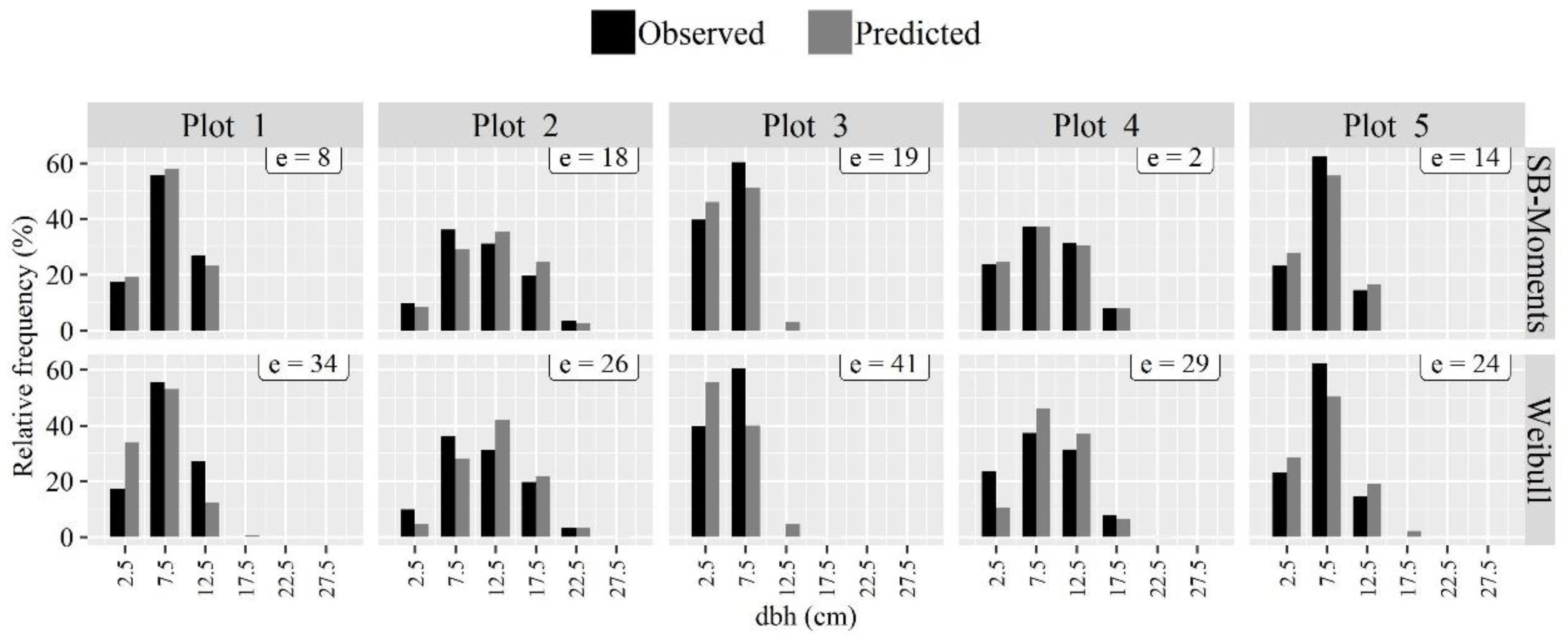
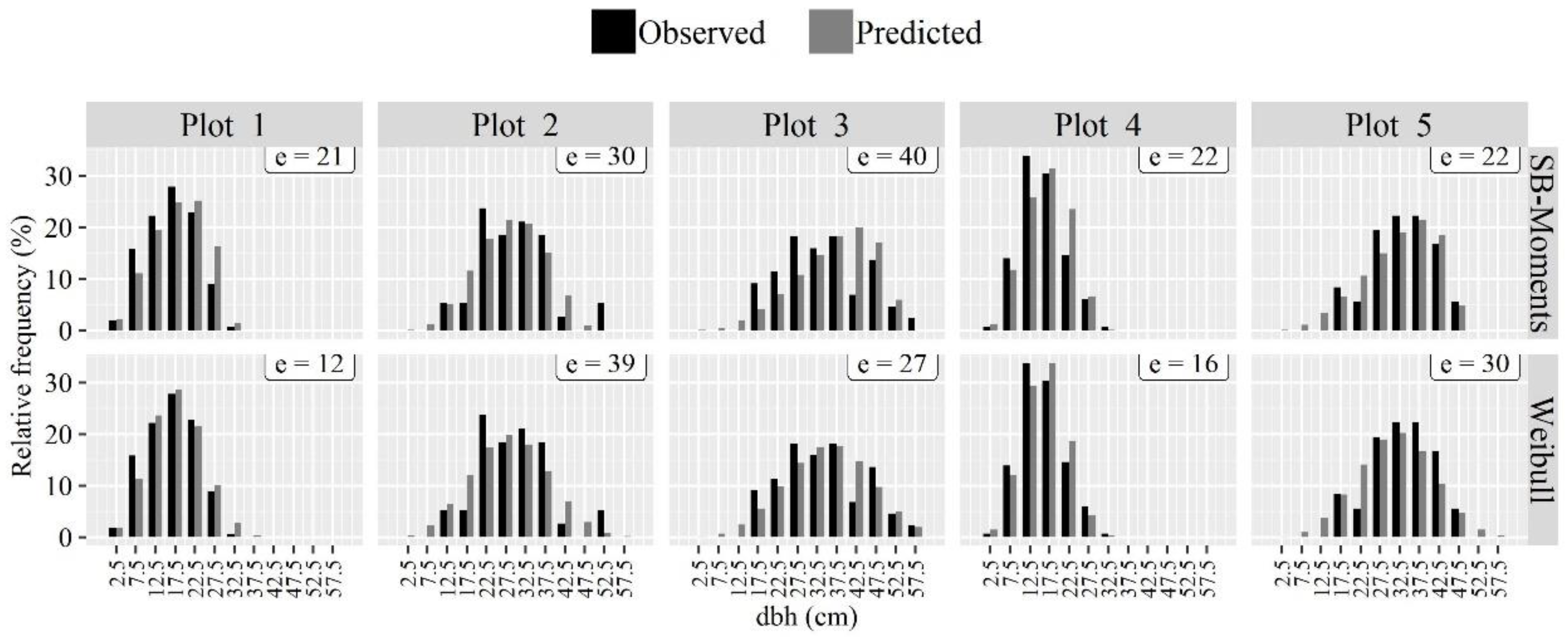
Since the S_B-Moments and Weibull presented good results for most accuracy assessments, their respective systems of equations are presented in Table 7. Both systems presented relatively good accuracy for their equations, with RMSE% lower than 16%, high r² (0.77–0.93) and a low Bias% (<3%, in absolute values). Examples of the diameter distributions produced by each of those approaches are presented in Figure 3 and Figure 4. The distributions over the E. globulus dataset showed that the S_B-Moments predictions are close to the observed frequencies for all exemplified plots (Figure 3). This fact is confirmed by their respective error indices, where the lowest values are obtained for the S_B-Moments, reflecting in smaller discrepancies than for the Weibull. As shown for the P. radiata dataset (Figure 4), the observed distributions are more complex and less smooth, with abrupt differences between the frequencies of consecutive dbh classes (e.g., Plots 2 and 3 in Figure 4). This fact explains the lower quality of the indicator values when assessing the distribution fittings. Nevertheless, the Weibull and S_B were able to reproduce those distributions satisfactorily, with a small advantage for the Weibull in most cases (e.g., Plots 1, 3, and 4 in Figure 4).

4. Discussion

This work performed a novel study by evaluating the capability of Johnson’s S_B to predict diameter distributions based on ALS data from two of the most common species used for forest plantations in the Iberian Peninsula: E. globulus and P. radiata. The results were different among the datasets, where the distributions resulted in better indicators when fitted over the E. globulus dataset. A plausible explanation for this difference is the distinction between the structure of the two forests and the adopted scanning properties. The eucalyptus ALS-data collection aimed at forest inventory while the pine flight was planned to produce high-resolution DTM for general applications in the country. Nationwide data have been applied to many forest-oriented studies, showing promising results in, e.g., Finland [62,63], Sweden [64], and Denmark [65]. Likewise, the Spanish survey proved to be a consistent data source for different forest applications [34,66,67,68,69,70]. However, nationwide ALS surveys are planned to reduce the flight costs so they present non-optimum scanning parameters for forest inventory, generally deriving low-density point clouds [71]. It is known that this characteristic has a negative impact on the forest modeling [72,73], so it is plausible that the models related to pine dataset have been influenced by the characteristics of the point density when compared to the ones derived from eucalyptus dataset.

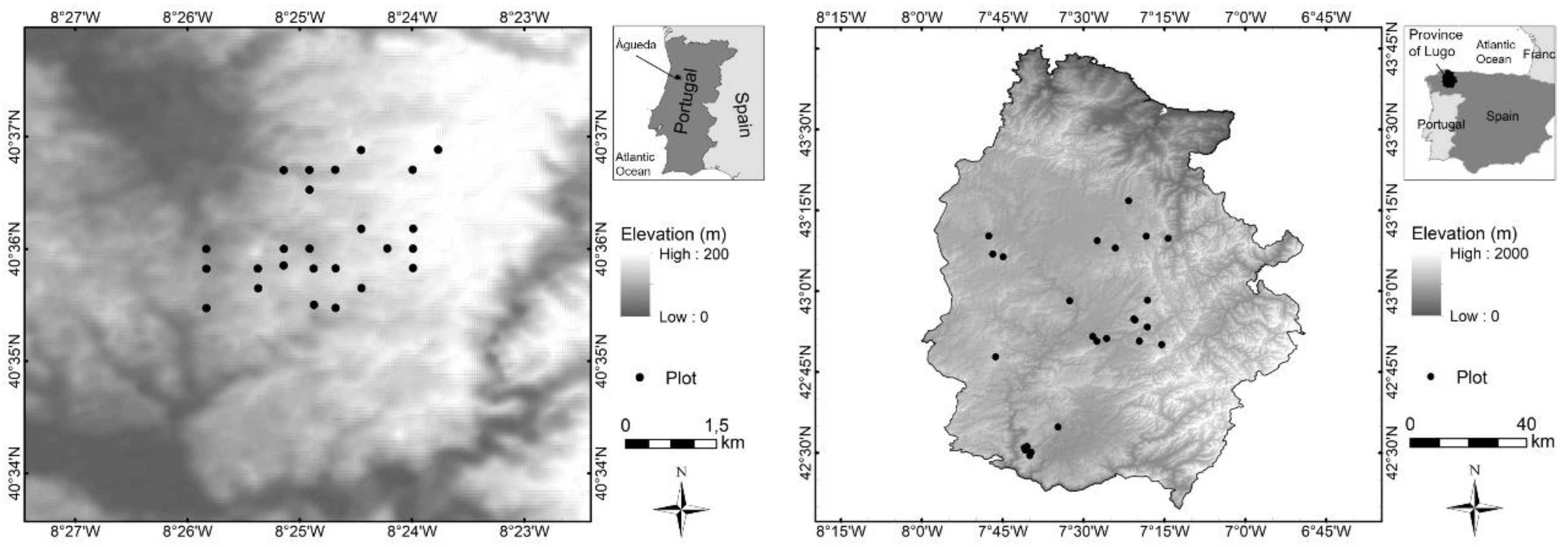
The pine dataset is located in a larger and more complex terrain when compared to the eucalyptus area (see Section 2.1). Thus, it is reasonable to consider this difference as a possible error source for the models since the terrain slope has a well-known influence on the accuracy of the ALS-derived DTM (e.g., [74,75]). However, the ABA has been commonly applied in steeped slopes with success (e.g., [76,77]) so it is not clear that the terrain complexity affects the forest models. Furthermore, the accuracy of the ALS surveys was relatively low (RMSE ≤ 0.25 m) so it is unlikely that the variation in the terrain had caused significant impact in the forest attribute predictions.

The S_B was highly sensitive to the input variables. Because of that, small deviations in the input predictions can result in changes in the parameters of the dbh distribution since they are interdependent in the fitting approaches (see Section 2.6). Therefore, the prediction errors can accumulate and affect the distribution even if the fitted equations have good performance. An example of those facts can be seen for S_B-3PR, which uses five stand variables as inputs in the parameter estimation and resulted in the worst performance for almost all assessments. On the other hand, the S_B-Moments and the S_B-Percentile use three stand variables each, while the Weibull has the advantage of using just two.

Each work involving the prediction of diameter distributions from ALS data has its particularities regarding the forest type, prediction approaches, or assessments, thus the comparative analysis among them is not straightforward. An exception is the work of Arias-Rodil [34], which used the same P. radiata dataset and LiDAR flight to estimate the diameter distribution through the two-parameter Weibull fitted also through parameter recovery approach. Our results show considerable improvement in relation to the Weibull distribution fitting; the acceptance by the KS test changes from 28% to 48% among plots. This fact was the result of the better equations to predict the stand variables used as predictors to estimate the distribution’s parameters, which use not two but up to three NHD metrics. If the S_B is taken into account, it is also considered as an improvement in the distribution’s prediction since it presented higher acceptance according to Arias-Rodil’s baseline, with 36% for the S_B-Moments.

Considering the best approaches of our work (S_B-Moments and Weibull), the mean error indices found could be considered low if compared to the literature. Maltamo et al. [10] found error index values of 50–60 for hybrid eucalyptus (E. urophilla x E. grandis) in Brazil using the two-parameter Weibull model. Other works involving boreal forests reported average indices varying 75–95 (“error2” of Maltamo et al. [18] [Editor1] ), 30–45 for diameter and basal area distributions [6], and 49–87 for just basal area distributions [7]. However, it should be highlighted that our dataset consists of homogeneous stands, thus, despite their variable structure, a lower modeling error was already expected.

According to the assessment through the growing stock prediction, the S_B-Moments presented a good indicator for the E. globulus data, where it performed slightly better than the Weibull. The Bias% of these estimations (≤2.0%, in absolute value) were comparable to the ones found by Gobakken and Næsset [6,7] [Editor2], with values below 4.8%, in absolute value. However, the Bias% values could be considered high in the case of the P. radiata data, varying 7–18% (in absolute value) for all approaches, although many of them presented reasonable RMSE% values and no significative differences between the predicted and ground reference values according to the paired t-test.

The deviations related to the N prediction are another source of error for the growing stock prediction assessment. The N is frequently reported as being one of the most difficult forest variables to be modeled from ALS data. In the related literature, it is common to find coefficients of determination (R², adjusted or not) of 0.50–0.82 in models with up to six metrics (e.g., [2,3,78]). One of the few studies with E. globulus plantations showed a low accuracy for the N equation (R² = 0.49), using 4 points m⁻² ALS data [79]. Woods et al. [80] suggested that this difficulty in modeling N could be bypassed if a high-point-density scanning is used. In our case, the E. globulus dataset has a relatively high density (9.5 points m⁻²) and the equation for the N was the least accurate, although its use is no longer discouraged. The N fitting for the P. radiata data, otherwise, presented a better accuracy even with a low pulse density (0.47 points m⁻²). In the case of availability of the tree density values of the stands, they could be applied to improve the growing stock prediction. Additionally, the modeling approaches could benefit from multisource data, such as multispectral images or multispectral ALS, which would contribute to improving predictions of the stand variables used as inputs in the estimation of the PDFs’ parameters.

The model transferability (see [77]) was not evaluated in this work so our results do not allow us to conclude about the efficiency of the models to predict attributes in stands from other regions. However, the models were developed using heterogeneous datasets in terms of stand age, density, and site index, and were assessed using a robust analysis. These features suggest that the developed models could be applied to E. globulus and P. radiata stands in the Iberian Peninsula. In the case of the absence of validation datasets to confirm such hypothesis, the replication of our methodology is recommended when the goal is to study different areas. Finally, this work filled the knowledge gap involving the Johnson’s S_B distribution and ALS approach and demonstrated that it allows obtaining accurate information about the forest horizontal structure to support decisions in forest management.

5. Conclusions

This work assessed the ability of the Johnson’s S_B and Weibull PDFs to model the diameter distributions of E. globulus and P. radiata plantations. In the studied areas, the S_B-Moments was the best approach to fit the S_B, while the S_B-3PR was the one providing the worse results. The performance of the S_B was comparable to the Weibull, presenting small advantages when applied to E. globulus data. S_B is very sensitive to the errors related to the predicted stand variables used to estimate the distribution parameters, so very accurate equations are required for their predictions.

References

1. Wulder, M.A.; White, J.C.; Nelson, R.F.; Næsset, E.; Ørka, H.O.; Coops, N.C.; Hilker, T.; Bater, C.W.; Gobakken, T. Lidar sampling for large-area forest characterization: A review. Remote. Sens. Environ. 2012, 121, 196–209. [Google Scholar] [CrossRef]
2. Næsset, E. Predicting forest stand characteristics with airborne scanning laser using a practical two-stage procedure and field data. Remote Sens. Environ. 2002, 80, 88–99. [Google Scholar] [CrossRef]
3. Næsset, E. Practical large-scale forest stand inventory using a small-footprint airborne scanning laser. Scand. J. For. Res. 2004, 19, 164–179. [Google Scholar] [CrossRef]
4. Burkhart, H.E.; Tomé, M. Modeling Forest Trees and Stands; Springer: Dordrecht, The Netherlands, 2012. [Google Scholar]
5. Maltamo, M.; Gobakken, T. Predicting tree diameter distributions. In Forestry Applycations of Airborne Laser Scanning: Concepts and Case Studies; Maltamo, M., Næsset, E., Vauhkonen, J., Eds.; Managing Forest Ecosystems; Springer: Dordrecht, The Netherlands, 2014; Volume 27, pp. 177–191. [Google Scholar]
6. Gobakken, T.; Næsset, E. Estimation of diameter and basal area distributions in coniferous forest by means of airborne laser scanner data. Scand. J. For. Res. 2004, 19, 529–542. [Google Scholar] [CrossRef]
7. Gobakken, T.; Næsset, E. Weibull and percentile models for lidar-based estimation of basal area distribution. Scand. J. For. Res. 2005, 20, 490–502. [Google Scholar] [CrossRef]
8. Maltamo, M.; Suvanto, A.; Packalén, P. Comparison of basal area and stem frequency diameter distribution modelling using airborne laser scanner data and calibration estimation. For. Ecol. Manag. 2007, 247, 26–34. [Google Scholar] [CrossRef]
9. Breidenbach, J.; Gläser, C.; Schmidt, M. Estimation of diameter distributions by means of airborne laser scanner data. Can. J. For. Res. 2008, 38, 1611–1620. [Google Scholar] [CrossRef]
10. Maltamo, M.; Mehtätalo, L.; Valbuena, R.; Vauhkonen, J.; Packalen, P. Airborne laser scanning for tree diameter distribution modelling: A comparison of different modelling alternatives in a tropical single-species plantation. Forestry 2018, 91, 121–131. [Google Scholar] [CrossRef]
11. Dudani, S.A. The distance-weighted k-nearest-neighbor rule. IEEE Trans. Syst. Man. Cybern. 1976, 325–327. [Google Scholar] [CrossRef]
12. Borders, B.E.; Souter, R.A.; Bailey, R.L.; Ware, K.D. Percentile-based distributions characterize forest stand tables. For. Sci. 1987, 33, 570–576. [Google Scholar]
13. Bollandsås, O.M.; Næsset, E. Estimating percentile-based diameter distributions in uneven-sized Norway spruce stands using airborne laser scanner data. Scand. J. For. Res. 2007, 22, 33–47. [Google Scholar] [CrossRef]
14. Packalén, P.; Maltamo, M. Estimation of species-specific diameter distributions using airborne laser scanning and aerial photographs. Can. J. For. Res. 2008, 38, 1750–1760. [Google Scholar] [CrossRef]
15. Maltamo, M.; Malinen, J.; Packalén, P.; Suvanto, A.; Kangas, J. Nonparametric estimation of stem volume using airborne laser scanning, aerial photography, and stand-register data. Can. J. For. Res. 2006, 36, 426–436. [Google Scholar] [CrossRef]
16. Xu, Q.; Hou, Z.; Maltamo, M.; Tokola, T. Calibration of area based diameter distribution with individual tree based diameter estimates using airborne laser scanning. ISPRS J. Photogramm. Remote Sens. 2014, 93, 65–75. [Google Scholar] [CrossRef]
17. Siipilehto, J.; Lindeman, H.; Vastaranta, M.; Yu, X.; Uusitalo, J. Reliability of the predicted stand structure for clear-cut stands using optional methods: Airborne laser scanning-based methods, smartphone-based forest inventory application Trestima and pre-harvest measurement tool EMO. Silva Fenn. 2016, 50. [Google Scholar] [CrossRef]
18. Maltamo, M.; Næsset, E.; Bollandsås, O.M.; Gobakken, T.; Packalén, P. Non-parametric prediction of diameter distributions using airborne laser scanner data. Scand. J. For. Res. 2009, 24, 541–553. [Google Scholar] [CrossRef]
19. Johnson, N.L. Systems of frequency curves generated by methods of translation. Biometrika 1949, 36, 149. [Google Scholar] [CrossRef]
20. Hafley, W.L.; Schreuder, H.T. Statistical distributions for fitting diameter and height data in even-aged stands. Can. J. For. Res. 1977, 7, 481–487. [Google Scholar] [CrossRef]
21. Barra, O.S.V.; Sanquetta, C.R.; Arce, J.E.; do Machado, S.A.; Corte, A.P.D. Proposta metodológica para o ajuste ótimo da distribuição diamétrica SB de Johnson. Rev. Árvore 2011, 35, 151–156. [Google Scholar] [CrossRef]
22. Fonseca, T.F.; Marques, C.P.; Parresol, B.R. Describing maritime pine diameter distributions with Johnson’s SB distribution using a new all-parameter recovery approach. For. Sci. 2009, 55, 367–373. [Google Scholar]
23. Gorgoso, J.J.; Rojo, A.; Cámara-Obregón, A.; Diéguez-Aranda, U. A comparison of estimation methods for fitting Weibull, Johnson’s SB and beta functions to Pinus pinaster, Pinus radiata and Pinus sylvestris stands in northwest Spain. For. Syst. 2012, 21, 446–459. [Google Scholar]
24. Kiviste, A.; Nilson, A.; Hordo, M.; Merenäkk, M. Diameter distribution models and height–diameter equations for Estonian forests. In Modelling Forest System; Amaro, A., Reed, D., Soares, P., Eds.; CABI: Wallingford, UK, 2003; p. 416. [Google Scholar]
25. Kudus, K.A.; Ahmad, M.I.; Lapongan, J. Nonlinear regression approach to estimating Johnson SB parameters for diameter data. Can. J. For. Res. 1999, 29, 310–314. [Google Scholar] [CrossRef]
26. De Moraes e Silva, V.S.; Soares, T.S.; Colpini, C.; Travagin, D.P.; Hosokawa, R.T.; Scolforo, J.R.S. Eucalyptus camaldulensis Dehnh. yield projection using johnson SB distribution. Rev. Árvore 2009, 33, 853–863. [Google Scholar]
27. Palahí, M.; Pukkala, T.; Blasco, E.; Trasobares, A. Comparison of beta, Johnson’s SB, Weibull and truncated Weibull functions for modeling the diameter distribution of forest stands in Catalonia (north-east of Spain). Eur. J. For. Res. 2007, 126, 563–571. [Google Scholar] [CrossRef]
28. Parresol, B.R. Recovering parameters of Johnson’s SB distribution; U.S. Department of Agriculture (USDA) Forest Service, Southern Research Station: Asheville, NC, USA, 2003.
29. Rennolls, K.; Wang, M. A new parameterization of Johnson’s SB distribution with application to fitting forest tree diameter data. Can. J. For. Res. 2005, 35, 575–579. [Google Scholar] [CrossRef]
30. Zhou, B.; McTague, J.P. Comparison and evaluation of five methods of estimation of the Johnson system parameters. Can. J. For. Res. 1996, 26, 928–935. [Google Scholar] [CrossRef]
31. Mateus, A.; Tomé, M. Modelling the diameter distribution of eucalyptus plantations with Johnson’s SB probability density function: Parameters recovery from a compatible system of equations to predict stand variables. Ann. For. Sci. 2011, 68, 325–335. [Google Scholar] [CrossRef]
32. Ferraz, A.; Mallet, C.; Jacquemoud, S.; Goncalves, G.R.; Tome, M.; Soares, P.; Pereira, L.G.; Bretar, F. Canopy density model: A new ALS-derived product to generate multilayer crown cover maps. IEEE Trans. Geosci. Remote Sens. 2015, 53, 6776–6790. [Google Scholar] [CrossRef]
33. Gonçalves, G.R.; Pereira, L.G. A thorough accuracy estimation of DTM produced from airborne full-waveform laser scanning data of unmanaged eucalypt plantations. IEEE Trans. Geosci. Remote Sens. 2012, 50, 3256–3266. [Google Scholar] [CrossRef]
34. Arias-Rodil, M.; Diéguez-Aranda, U.; Álvarez-González, J.G.; Pérez-Cruzado, C.; Castedo-Dorado, F.; González-Ferreiro, E. Modeling diameter distributions in radiata pine plantations in Spain with existing countrywide LiDAR data. Ann. For. Sci. 2018, 75, 36. [Google Scholar] [CrossRef]
35. Castedo-Dorado, F.; Gómez-Vázquez, I.; Fernandes, P.M.; Crecente-Campo, F. Shrub fuel characteristics estimated from overstory variables in NW Spain pine stands. For. Ecol. Manage. 2012, 275, 130–141. [Google Scholar] [CrossRef]
36. Autoridade Florestal Nacional. Instruções para o Trabalho de Campo do Inventário Florestal Nacional—IFN 2005/2006; Direção de Unidade de Gestão Florestal, Divisão para a Intervenção Florestal: Lisboa, Portugal, 2009. [Google Scholar]
37. Prodan, M. Holzmesslehre; Sauerländer’s Verlag: Frankfurt, Germany, 1965. [Google Scholar]
38. Ferraz, A.; Bretar, F.; Jacquemoud, S.; Gonçalves, G.; Pereira, L.; Tomé, M.; Soares, P. 3-D mapping of a multi-layered Mediterranean forest using ALS data. Remote Sens. Environ. 2012, 121, 210–223. [Google Scholar] [CrossRef]
39. Castedo-Dorado, F.; Diéguez-Aranda, U.; Álvarez-González, J.G. A growth model for Pinus radiata D. Don stands in north-western Spain. Ann. For. Sci. 2007, 64, 453–465. [Google Scholar] [CrossRef]
40. Gómez-Vázquez, I.; Crecente-Campo, F.; Diéguez-Aranda, U.; Castedo-Dorado, F. Modelling canopy fuel variables in Pinus pinaster Ait. and Pinus radiata D. Don stands in northwestern Spain. Ann. For. Sci. 2013, 70, 161–172. [Google Scholar] [CrossRef]
41. Tomé, M.; Tomé, J.; Ribeiro, F.; Faias, S. Equações de volume total, volume percentual e de perfil do tronco para Eucalyptus globulus Labill. em Portugal. Silva Lusit. 2007, 15, 25–39. [Google Scholar]
42. Diéguez-Aranda, U.; Alboreca, A.R.; Castedo-Dorado, F.; González, J.G.Á.; Barrio-Anta, M.; Crecente-Campo, F.; González, J.M.G.; Pérez-Cruzado, C.; Soalleiro, R.R.; López-Sánchez, C.A.; et al. Herramientas selvícolas para la gestión forestal sostenible en Galicia; Dirección Xeral de Montes, Xunta de Galicia; Tórculo Artes Gráficas, S.A: Lugo, Spain, 2009. [Google Scholar]
43. McGaughey, R. FUSION/LDV: Software for LIDAR data analysis and visualization, v3.60+. United States Dep. Agric. For. Serv. Pacific Northwest Res. Stn. 2018, 211. [Google Scholar]
44. Kraus, K.; Pfeifer, N. Determination of terrain models in wooded areas with airborne laser scanner data. ISPRS J. Photogramm. Remote Sens. 1998, 53, 193–203. [Google Scholar] [CrossRef]
45. Wang, Q.J. Direct sample estimators of L moments. Water Resour. Res. 1996, 32, 3617–3619. [Google Scholar] [CrossRef]
46. Siipilehto, J.; Sarkkola, S.; Mehtätalo, L. Comparing regression estimation techniques when predicting diameter distributions of scots pine on drained peatlands. Silva Fenn. 2007, 41, 333–349. [Google Scholar] [CrossRef] [Green Version]
47. Scolforo, J.R.S.; Tabai, F.C.V.; de Macedo, R.L.G.; Acerbi, F.W.; de Assis, A.L. SB distribution’s accuracy to represent the diameter distribution of Pinus taeda, through five fitting methods. For. Ecol. Manage. 2003, 175, 489–496. [Google Scholar] [CrossRef]
48. Knoebel, B.; Burkhart, H. A bivariate distribution approach to modeling forest diameter distributions at two points in time. Biometrics 1991, 47, 241–253. [Google Scholar] [CrossRef]
49. Parresol, B.R.; Fonseca, T.; Marques, C. Numerical details and SAS programs for parameter recovery of the SB distribution; Res. Pap. SRS–122; U.S. Department of Agriculture (USDA) Forest Service, Southern Research Station: Asheville, NC, USA, 2010.
50. R Core Team R: A Language and Environment for Statistical Computing. Available online: https://www.r-project.org/ (accessed on 12 September 2019).
51. Elzhov, T.V.; Mullen, K.M.; Spiess, A.-N.; Bolker, B. minpack.lm: R Interface to the Levenberg-Marquardt Nonlinear Least-squares Algorithm Found in MINPACK, Plus Support for Bounds. Available online: https://cran.r-project.org/package=minpack.lm (accessed on 12 September 2019).
52. Bailey, R.L.; Dell, R. Quantifying diameter distributions with the weibull function. For. Sci. 1972, 19, 97–104. [Google Scholar]
53. Newby, M.J. The properties of moment estimators for the weibull distribution based on the sample Coefficient of Variation. Technometrics 1980, 22, 187. [Google Scholar] [CrossRef]
54. Burk, T.E.; Newberry, J.D. Notes: A simple algorithm for moment-based recovery of weibull distribution parameters. For. Sci. 1984, 30, 329–332. [Google Scholar]
55. Myers, R.H. Classical and Modern Regression with Applications; Duxbury Press: Boston, MA, USA, 1989. [Google Scholar]
56. Fox, J.; Weisberg, S. An R Companion to Applied Regression. Available online: https://socialsciences.mcmaster.ca/jfox/Books/Companion/ (accessed on 12 September 2019).
57. Zellner, A.; Theil, H. Three-stage least squares: Simultaneous estimation of simultaneous equations. Econometrica. 1962, 30, 54–78. [Google Scholar] [CrossRef]
58. Henningsen, A.; Hamann, J.D. Systemfit: A package for estimating systems of simultaneous equations in R. J. Stat. Softw. 2007, 23, 1–40. [Google Scholar] [CrossRef] [Green Version]
59. Lilliefors, H.W. On the Kolmogorov-Smirnov test for normality with mean and variance unknown. J. Am. Stat. Assoc. 1967, 62, 399–402. [Google Scholar] [CrossRef]
60. Siipilehto, J. A comparison of two parameter prediction methods for stand structure in Finland. Silva Fenn. 2000, 34, 331–349. [Google Scholar] [CrossRef] [Green Version]
61. Reynolds, M.R.; Burk, T.E.; Huang, W.-C. Goodness-of-fit tests and model selection procedures for diameter distribution models. For. Sci. 1988, 34, 373–399. [Google Scholar]
62. Kotivuori, E.; Korhonen, L.; Packalen, P. Nationwide airborne laser scanning based models for volume, biomass and dominant height in Finland. Silva Fenn. 2016, 50, 1–28. [Google Scholar] [CrossRef] [Green Version]
63. Kotivuori, E.; Maltamo, M.; Korhonen, L.; Packalen, P. Calibration of nationwide airborne laser scanning based stem volume models. Remote Sens. Environ. 2018, 210, 179–192. [Google Scholar] [CrossRef]
64. Nilsson, M.; Nordkvist, K.; Jonzén, J.; Lindgren, N.; Axensten, P.; Wallerman, J.; Egberth, M.; Larsson, S.; Nilsson, L.; Eriksson, J. A nationwide forest attribute map of Sweden predicted using airborne laser scanning data and field data from the National Forest Inventory. Remote Sens. Environ. 2017, 194, 447–454. [Google Scholar] [CrossRef]
65. Nord-Larsen, T.; Riis-Nielsen, T. Developing an airborne laser scanning dominant height model from a countrywide scanning survey and national forest inventory data. Scand. J. For. Res. 2010, 25, 262–272. [Google Scholar] [CrossRef]
66. Guerra-Hernández, J.; Tomé, M.; González-Ferreiro, E. Using low density LiDAR data to map Mediterranean forest characteristics by means of an area-based approach and height threshold analysis. Rev. Teledetección 2016, 103–107. [Google Scholar]
67. González-Ferreiro, E.; Arellano-Pérez, S.; Castedo-Dorado, F.; Hevia, A.; Vega, J.A.; Vega-Nieva, D.; Álvarez-González, J.G.; Ruiz-González, A.D. Modelling the vertical distribution of canopy fuel load using national forest inventory and low-density airbone laser scanning data. PLoS ONE 2017, 12, e0176114. [Google Scholar] [CrossRef]
68. Montealegre, A.L.; Lamelas, M.T.; de la Riva, J.; García-Martín, A.; Escribano, F. Use of low point density ALS data to estimate stand-level structural variables in Mediterranean Aleppo pine forest. Forestry 2016, 89, 373–382. [Google Scholar] [CrossRef] [Green Version]
69. Montealegre, A.; Lamelas, M.; Tanase, M.; de la Riva, J. Forest fire severity assessment using ALS data in a mediterranean environment. Remote Sens. 2014, 6, 4240–4265. [Google Scholar] [CrossRef] [Green Version]
70. González-Ferreiro, E.; Diéguez-Aranda, U.; Crecente-Campo, F.; Barreiro-Fernández, L.; Miranda, D.; Castedo-Dorado, F. Modelling canopy fuel variables for Pinus radiata D. Don in NW Spain with low-density LiDAR data. Int. J. Wildl. Fire 2014, 23, 350–362. [Google Scholar] [CrossRef]
71. Ahokas, E.; Yu, X.; Oksanen, J.; Kaartinen, H.; Model, D.T. Optimization of the Scanning Angle for Countrywide. In Proceedings of the Laser Scanning; Vosselman, G., Brenner, C., Hyyppä, J., Eds.; International Society for Photogrammetry and Remote Sensing (ISPRS): Enschede, The Netherlands, 2005; pp. 115–119. [Google Scholar]
72. Jakubowski, M.K.; Guo, Q.; Kelly, M. Tradeoffs between lidar pulse density and forest measurement accuracy. Remote Sens. Environ. 2013, 130, 245–253. [Google Scholar] [CrossRef]
73. Hansen, E.H.; Gobakken, T.; Næsset, E. Effects of pulse density on digital terrain models and canopy metrics using airborne laser scanning in a tropical rainforest. Remote Sens. 2015, 7, 8453–8468. [Google Scholar] [CrossRef] [Green Version]
74. Stereńczak, K.; Ciesielski, M.; Bałazy, R.; Zawiła-Niedźwiecki, T. Comparison of various algorithms for DTM interpolation from LIDAR data in dense mountain forests. Eur. J. Remote Sens. 2016, 49, 599–621. [Google Scholar] [CrossRef]
75. Liu, X. Airborne LiDAR for DEM generation: Some critical issues. Prog. Phys. Geogr. Earth Environ. 2008, 32, 31–49. [Google Scholar]
76. Corona, P.; Cartisano, R.; Salvati, R.; Chirici, G.; Floris, A.; di Martino, P.; Marchetti, M.; Scrinzi, G.; Clementel, F.; Travaglini, D. Airborne laser scanning to support forest resource management under alpine, temperate and mediterranean environments in Italy. Eur. J. Remote Sens. 2012, 45, 27–37. [Google Scholar] [CrossRef] [Green Version]
77. Tompalski, P.; White, J.C.; Coops, N.C.; Wulder, M.A. Demonstrating the transferability of forest inventory attribute models derived using airborne laser scanning data. Remote Sens. Environ. 2019, 227, 110–124. [Google Scholar] [CrossRef]
78. Thomas, V.; Oliver, R.D.; Lim, K.; Woods, M. LiDAR and Weibull modeling of diameter and basal area. For. Chron. 2008, 84, 866–875. [Google Scholar] [CrossRef] [Green Version]
79. Gonçalves-Seco, L.; González-Ferreiro, E.; Diéguez-Aranda, U.; Fraga-Bugallo, B.; Crecente, R.; Miranda, D. Assessing the attributes of high-density Eucalyptus globulus stands using airborne laser scanner data. Int. J. Remote Sens. 2011, 32, 9821–9841. [Google Scholar] [CrossRef]
80. Woods, M.; Lim, K.; Treitz, P. Predicting forest stand variables from LiDAR data in the Great Lakes—St. Lawrence forest of Ontario. For. Chron. 2008, 84, 827–839. [Google Scholar] [CrossRef] [Green Version]
Figure 1. Study areas of: (left) eucalyptus stands; and (right) pine stands.
Remotesensing 11 02792 g001
Figure 2. Data dispersion over the β1 and β2 coefficients computed for the tree dbh within plots.
Remotesensing 11 02792 g002
Figure 3. SB-Moments and Weibull distributions and error indices (e) for five plots of the eucalyptus dataset.
Remotesensing 11 02792 g003
Figure 4. SB-Moments and Weibull diameter and error indices (e) for five plots of the pine dataset.
Remotesensing 11 02792 g004