Mobile Laser Scanning for Estimating Tree Stem Diameter Using Segmentation and Tree Spine Calibration


Abstract
:
1. Introduction
2. Material
2.1. Laser Scanner
2.2. Inertial Navigation System
2.3. Data Logging and Time Synchronization
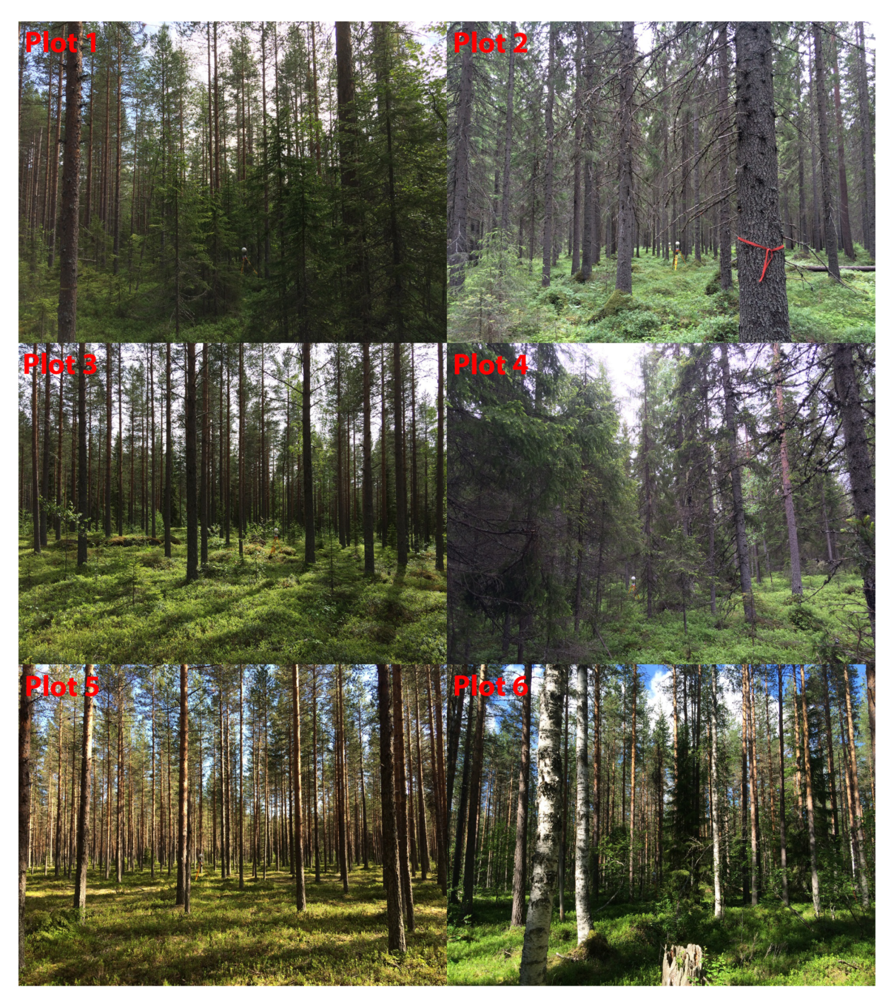
2.4. Validation Data
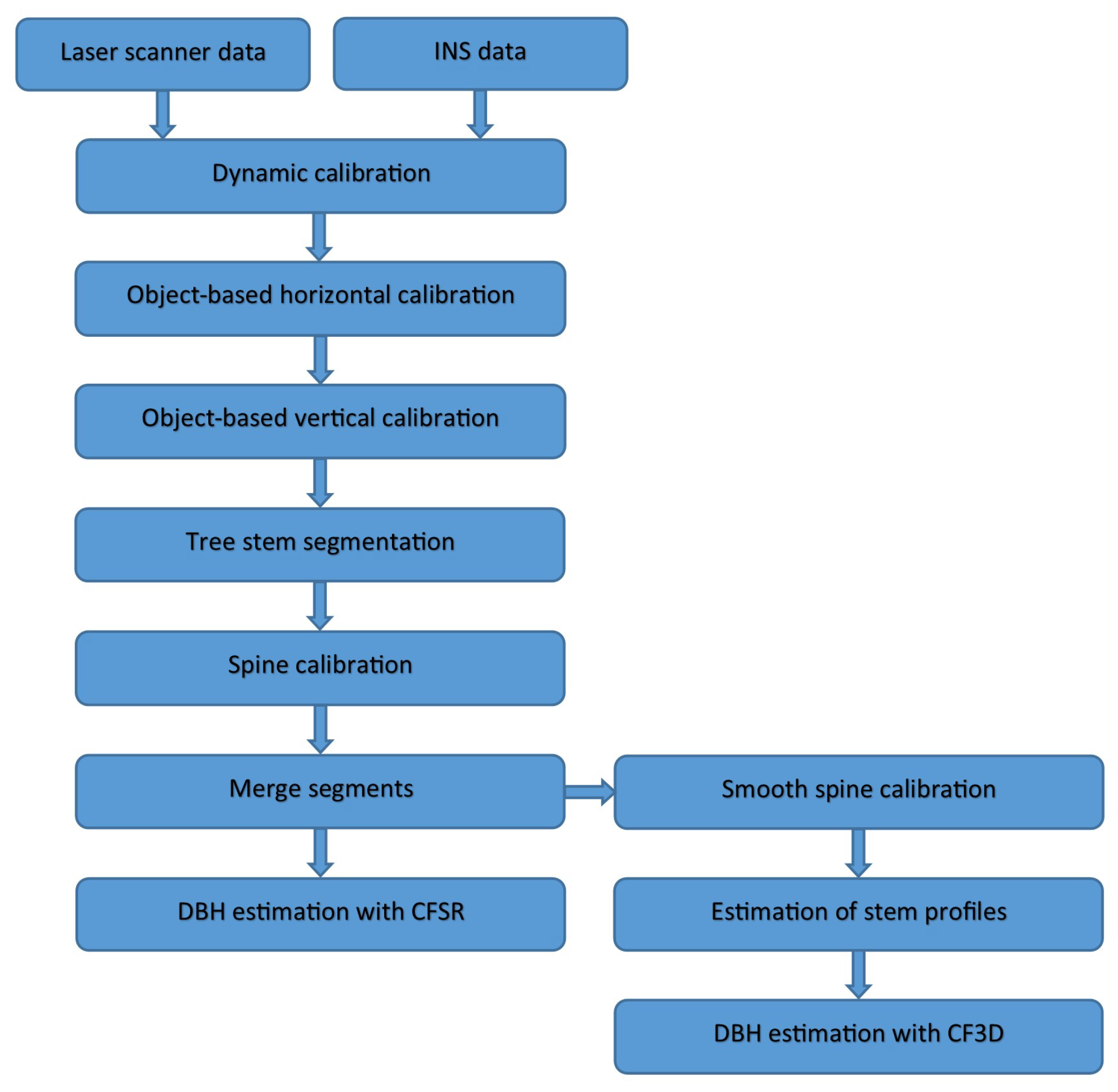
3. Methods
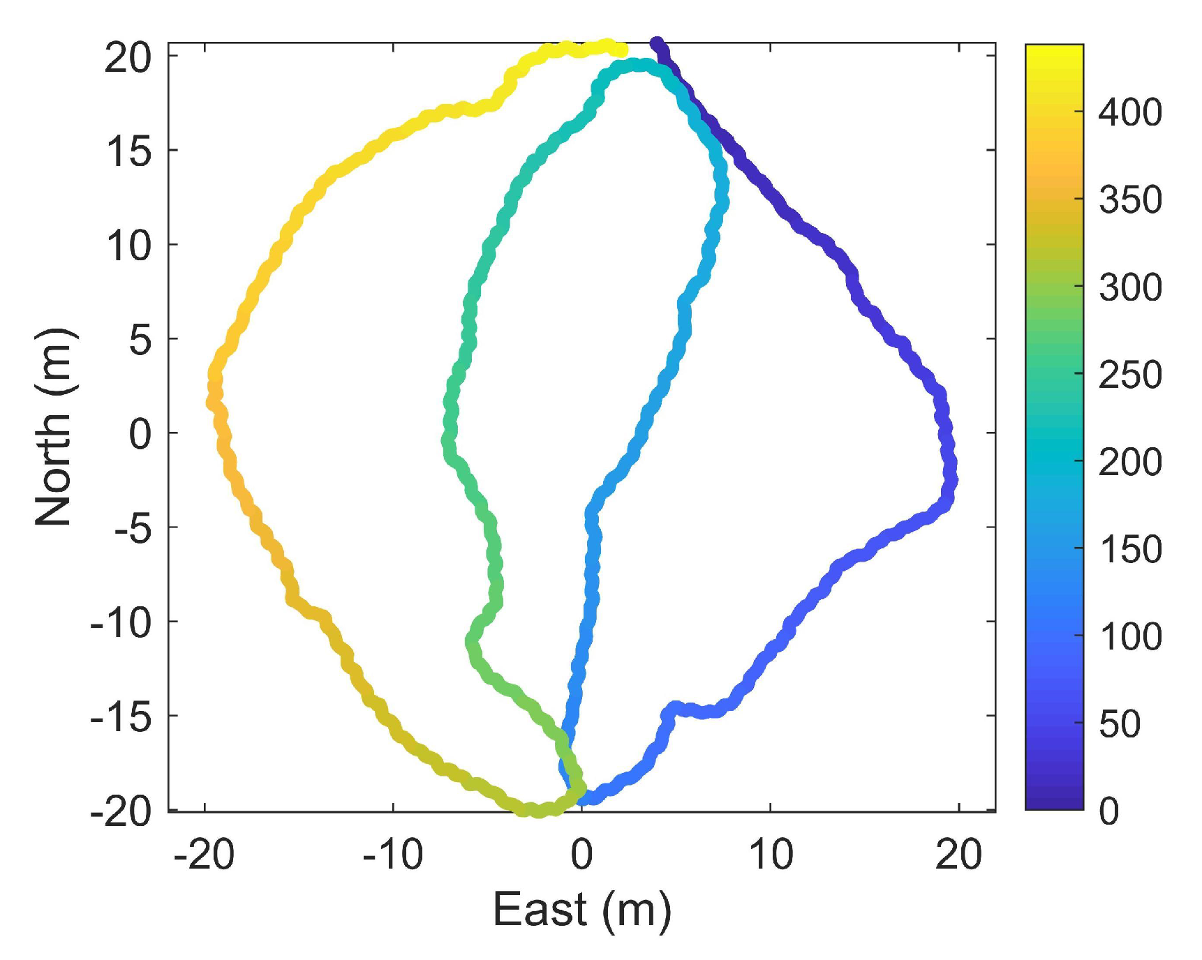
3.1. Dynamic Calibration
3.2. Horizontal Object-Based Calibration
3.3. Vertical Object-Based Calibration
3.4. Tree Stem Segmentation
| Algorithm 1 Segmentation |
|
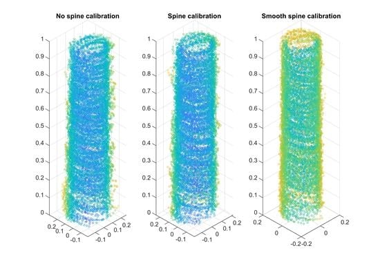
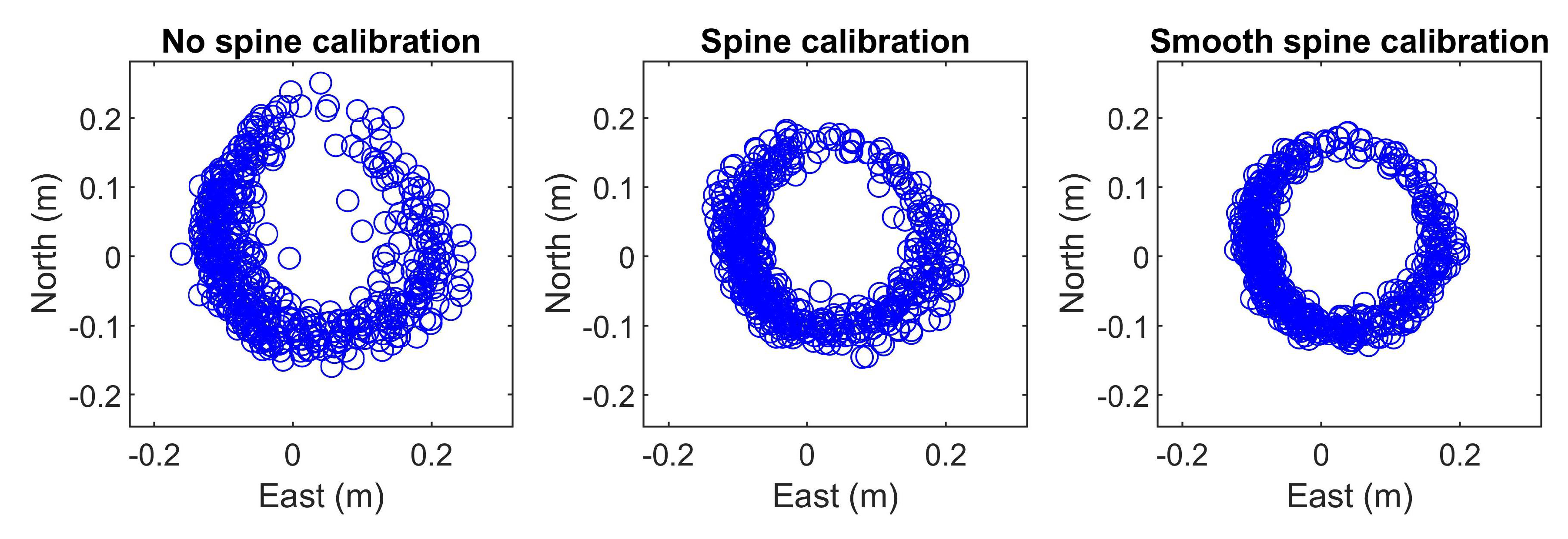
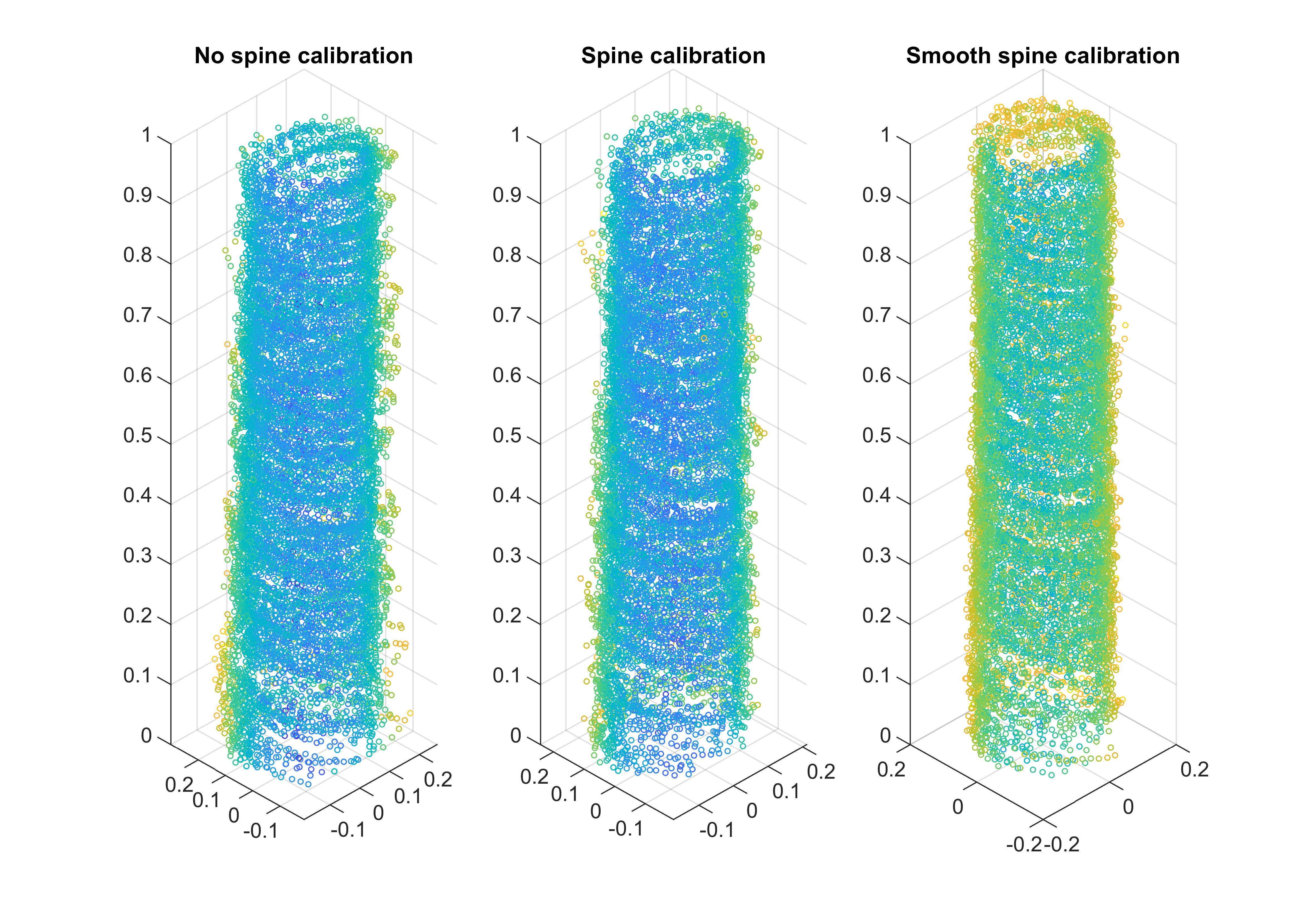
3.5. Spine Calibration
| Algorithm 2 Spine calibration |
|
3.6. Merge Segments
3.7. Smooth Spine Calibration
| Algorithm 3 Smooth spine calibration |
|
3.8. Estimation of Stem Profiles
3.9. Ground Elevation Model
3.10. Circle Fit Within Scan Revolutions (CFSR)
3.11. Circle Fit of 3D Point Cloud (CF3D)
3.12. Validation
4. Results
5. Discussion
6. Conclusions
Author Contributions
Funding
Acknowledgments
Conflicts of Interest
References
- Thies, M.; Pfeifer, N.; Winterhalder, D.; Gorte, B.G.H. Three-dimensional reconstruction of stems for assessment of taper, sweep and lean based on laser scanning of standing trees. Scand. J. For. Res. 2004, 19, 571–581. [Google Scholar] [CrossRef]
- Liang, X.; Kukko, A.; Kaartinen, H.; Hyyppä, J.; Yu, X.; Jaakkola, A.; Wang, Y. Possibilities of a Personal Laser Scanning System for Forest Mapping and Ecosystem Services. Sensors 2014, 14, 1228–1248. [Google Scholar] [CrossRef]
- Bosse, M.; Zlot, R.; Flick, P. Zebedee: Design of a spring-mounted 3-d range sensor with application to mobile mapping. IEEE Trans. Robot. 2012, 28, 1104–1119. [Google Scholar] [CrossRef]
- Zhang, J.; Singh, S. LOAM: Lidar Odometry and Mapping in Real-time. In Robotics: Science and Systems; Citeseer: Princeton, NJ, USA, 2014; Volume 2. [Google Scholar]
- Tang, J.; Chen, Y.; Kukko, A.; Kaartinen, H.; Jaakkola, A.; Khoramshahi, E.; Hakala, T.; Hyyppä, J.; Holopainen, M.; Hyyppä, H. SLAM-aided stem mapping for forest inventory with small-footprint mobile LiDAR. Forests 2015, 6, 4588–4606. [Google Scholar] [CrossRef]
- Qian, C.; Liu, H.; Tang, J.; Chen, Y.; Kaartinen, H.; Kukko, A.; Zhu, L.; Liang, X.; Chen, L.; Hyyppä, J. An integrated GNSS/INS/LiDAR-SLAM positioning method for highly accurate forest stem mapping. Remote Sens. 2016, 9, 3. [Google Scholar] [CrossRef]
- Kukko, A.; Kaijaluoto, R.; Kaartinen, H.; Lehtola, V.V.; Jaakkola, A.; Hyyppä, J. Graph SLAM correction for single scanner MLS forest data under boreal forest canopy. ISPRS J. Photogramm. Remote Sens. 2017, 132, 199–209. [Google Scholar] [CrossRef]
- Liang, X.; Kukko, A.; Hyyppä, J.; Lehtomäki, M.; Pyörälä, J.; Yu, X.; Kaartinen, H.; Jaakkola, A.; Wang, Y. In-situ measurements from mobile platforms: An emerging approach to address the old challenges associated with forest inventories. ISPRS J. Photogramm. Remote Sens. 2018, 143, 97–107. [Google Scholar] [CrossRef]
- Oveland, I.; Hauglin, M.; Gobakken, T.; Næsset, E.; Maalen-Johansen, I. Automatic estimation of tree position and stem diameter using a moving terrestrial laser scanner. Remote Sens. 2017, 9, 350. [Google Scholar] [CrossRef]
- Oveland, I.; Hauglin, M.; Giannetti, F.; Schipper Kjørsvik, N.; Gobakken, T. Comparing three different ground based laser scanning methods for tree stem detection. Remote Sens. 2018, 10, 538. [Google Scholar] [CrossRef]
- Holmgren, J.; Tulldahl, H.M.; Nordlöf, J.; Nyström, M.; Olofsson, K.; Rydell, J.; Willén, E. Estimation of tree position and stem diameter using simultaneous localization and mapping with data from a backpack-mounted laser scanner. Int. Arch. Photogramm. Remote Sens. Spat. Inf. Sci. 2017, XLII-3/W3, 59–63. [Google Scholar] [CrossRef]
- Olofsson, K.; Holmgren, J. Single Tree Stem Profile Detection Using Terrestrial Laser Scanner Data, Flatness Saliency Features and Curvature Properties. Forests 2016, 7, 207. [Google Scholar] [CrossRef]
- Olofsson, K.; Lindberg, E.; Holmgren, J. A method for linking field-surveyed and aerial-detected single trees using cross correlation of position images and the optimization of weighted tree list graphs. In Proceedings of the SilviLaser 2008, 8th International Conference on LiDAR Applications in Forest Assessment and Inventory, Edinburgh, UK, 17–19 September 2008; Hill, R., Rosette, J., Suarez, J., Eds.; pp. 95–104. [Google Scholar]
- Tulldahl, M.; Rydell, J.; Holmgren, J.; Nordlöf, J.; Willén, E. Lidar-based positioning in forest environments. In Proceedings of the Electro-Optical Remote Sensing XIII, Strasbourg, France, 9–12 September 2019; Kamerman, G., Steinvall, O., Eds.; International Society for Optics and Photonics, SPIE: Bellingham, WA, USA, 2019; Volume 11160, pp. 32–47. [Google Scholar] [CrossRef]
- Tulldahl, H.M.; Larsson, H. Lidar on small UAV for 3D mapping. In Proceedings of the SPIE Security+ Defence, Amsterdam, The Netherlands, 22–25 September 2014; International Society for Optics and Photonics: Bellingham, WA, USA, 2014; pp. 925009-1–925009–14. [Google Scholar]
- Tulldahl, H.M.; Bissmarck, F.; Larsson, H.; Grönwall, C.; Tolt, G. Accuracy evaluation of 3D lidar data from small UAV. In Proceedings of the SPIE Security+ Defence, Toulouse, France, 21–24 September 2015; International Society for Optics and Photonics: Bellingham, WA, USA, 2015; pp. 964903-1–964903–11. [Google Scholar]
- Armijo, L. Minimization of functions having Lipschitz continuous first partial derivatives. Pac. J. Math. 1966, 16, 1–3. [Google Scholar] [CrossRef]
- Elmqvist, M.; Jungert, E.; Lantz, F.; Persson, Å.; Söderman, U. Terrain modelling and analysis using laser scanner data. Int. Arch. Photogramm. Remote Sens. Spat. Inf. Sci. 2001, 34, 219–226. [Google Scholar]
- Forsman, M.; Börlin, N.; Olofsson, K.; Reese, H.; Holmgren, J. Bias of cylinder diameter estimation from ground-based laser scanners with different beam widths: A simulation study. ISPRS J. Photogramm. Remote Sens. 2018, 135, 84–92. [Google Scholar] [CrossRef]
- Forsman, M.; Holmgren, J.; Olofsson, K. Tree Stem Diameter Estimation from Mobile Laser Scanning Using Line-Wise Intensity-Based Clustering. Forests 2016, 7, 206. [Google Scholar] [CrossRef]
- Liang, X.; Hyyppä, J.; Kukko, A.; Kaartinen, H.; Jaakkola, A.; Yu, X. The Use of a Mobile Laser Scanning System for Mapping Large Forest Plots. IEEE Geosci. Remote Sens. Lett. 2014, 11, 1504–1508. [Google Scholar] [CrossRef]


| PLOT | RMSE (mm) | Rel. RMSE (%) | Bias (mm) | Rel. Bias (%) | ||||
|---|---|---|---|---|---|---|---|---|
| CFSR | CF3D | CFSR | CF3D | CFSR | CF3D | CFSR | CF3D | |
| 1 | 17 | 10 | 9 | 5 | 6 | 1 | 3 | 1 |
| 2 | 15 | 15 | 5 | 5 | 8 | −2 | 3 | −1 |
| 3 | 8 | 9 | 3 | 4 | 4 | −3 | 2 | −1 |
| 4 | 12 | 12 | 6 | 5 | 4 | 0 | 2 | 0 |
| 5 | 7 | 7 | 4 | 4 | 4 | 3 | 2 | 2 |
| 6 | 9 | 9 | 5 | 4 | −1 | −4 | −1 | −2 |
| PLOT | RMSE (mm) | Rel. RMSE (%) | Bias (mm) | Rel. Bias (%) | ||||
|---|---|---|---|---|---|---|---|---|
| CFSR | CF3D | CFSR | CF3D | CFSR | CF3D | CFSR | CF3D | |
| 1 | 18 | 19 | 10 | 10 | 7 | 5 | 4 | 3 |
| 2 | 15 | 15 | 5 | 5 | 8 | −1 | 3 | 0 |
| 3 | 8 | 9 | 3 | 4 | 4 | −3 | 2 | −1 |
| 4 | 28 | 45 | 14 | 22 | 11 | 19 | 5 | 9 |
| 5 | 7 | 7 | 4 | 4 | 4 | 3 | 2 | 2 |
| 6 | 24 | 41 | 14 | 23 | 3 | 7 | 2 | 4 |
| PLOT | Link A (%) | Link B (%) | Link C (%) | Commission (%) | Manual | ||||
|---|---|---|---|---|---|---|---|---|---|
| CFSR | CF3D | CFSR | CF3D | CFSR | CF3D | CFSR | CF3D | ||
| 1 | 50 | 46 | 52 | 51 | 59 | 59 | 6 | 7 | 171 |
| 2 | 79 | 76 | 79 | 79 | 95 | 95 | 3 | 3 | 63 |
| 3 | 93 | 93 | 93 | 93 | 100 | 100 | 2 | 3 | 59 |
| 4 | 46 | 33 | 62 | 62 | 68 | 68 | 4 | 4 | 132 |
| 5 | 89 | 86 | 89 | 89 | 98 | 98 | 2 | 2 | 122 |
| 6 | 62 | 49 | 73 | 73 | 79 | 79 | 5 | 5 | 169 |
© 2019 by the authors. Licensee MDPI, Basel, Switzerland. This article is an open access article distributed under the terms and conditions of the Creative Commons Attribution (CC BY) license (http://creativecommons.org/licenses/by/4.0/).
Share and Cite
Holmgren, J.; Tulldahl, M.; Nordlöf, J.; Willén, E.; Olsson, H. Mobile Laser Scanning for Estimating Tree Stem Diameter Using Segmentation and Tree Spine Calibration. Remote Sens. 2019, 11, 2781. https://doi.org/10.3390/rs11232781
Holmgren J, Tulldahl M, Nordlöf J, Willén E, Olsson H. Mobile Laser Scanning for Estimating Tree Stem Diameter Using Segmentation and Tree Spine Calibration. Remote Sensing. 2019; 11(23):2781. https://doi.org/10.3390/rs11232781
Chicago/Turabian StyleHolmgren, Johan, Michael Tulldahl, Jonas Nordlöf, Erik Willén, and Håkan Olsson. 2019. "Mobile Laser Scanning for Estimating Tree Stem Diameter Using Segmentation and Tree Spine Calibration" Remote Sensing 11, no. 23: 2781. https://doi.org/10.3390/rs11232781
APA StyleHolmgren, J., Tulldahl, M., Nordlöf, J., Willén, E., & Olsson, H. (2019). Mobile Laser Scanning for Estimating Tree Stem Diameter Using Segmentation and Tree Spine Calibration. Remote Sensing, 11(23), 2781. https://doi.org/10.3390/rs11232781