Abstract
This paper presents a novel approach for automatically detecting land cover changes from multitemporal high-resolution remote sensing images in the deep feature space. This is accomplished by using multitemporal deep feature collaborative learning and a semi-supervised Chan–Vese (SCV) model. The multitemporal deep feature collaborative learning model is developed to obtain the multitemporal deep feature representations in the same high-level feature space and to improve the separability between changed and unchanged patterns. The deep difference feature map at the object-level is then extracted through a feature similarity measure. Based on the deep difference feature map, the SCV model is proposed to detect changes in which labeled patterns automatically derived from uncertainty analysis are integrated into the energy functional to efficiently drive the contour towards accurate boundaries of changed objects. The experimental results obtained on the four data sets acquired by different high-resolution sensors corroborate the effectiveness of the proposed approach.
1. Introduction
Land cover change information is extremely important for the study of global climate change, biodiversity, environmental monitoring, and national resources management [1,2,3,4]. In recent decades, change detection (CD) using multi-temporal remote sensing datasets to quantify the changes and temporal effects on the Earth’s surface have become a research hotspot [5,6]. Along with the rapid development of Earth observing technology, vast amounts of CD methodologies from remote sensing imagery have been developed and newer techniques are still emerging [6,7,8].
In the literature, the developed CD approaches can be classified into two categories, namely post-classification comparison and direct comparison [9,10]. Post-classification comparison is performed on multitemporal images to independently classify pixels, and then the classified maps are compared for change analysis [11,12,13]. The direct comparison of multispectral images is generally achieved by two steps: generating a difference feature map containing change magnitudes and analyzing the feature map to detect the changed areas [14,15,16]. Layer arithmetic operations (e.g., image differencing and change vector analysis [14]) and data transformation (e.g., principle component analysis [17] and histogram trend similarity [7]) can be used to generate the difference feature map. Then, analyzing methods for the feature map including thresholding, clustering, image segmentation, and machine learning are performed to discriminate changed and unchanged areas [6]. Direct comparison approaches based on the difference feature map have been widely implemented to automatically detect changes from multitemporal remote sensing data without the need for any prior information.
Based on the unit of analysis, these CD approaches can be categorized into pixel-based and object-based methods [18,19,20,21,22]. Pixel-based approaches mainly include the expectation maximization algorithm (EM), the fuzzy C-means (FCM), and active contour models (ACMs) [10,23]. The Chan–Vese (CV) model reduces the complexity of the optimization problem of ACMs and has been extensively studied in pixel-based CD approaches [24,25,26]. The local uncertainty of pixels was incorporated into the CV model to construct energy constraints in [27] to improve the accuracy of CD results and the computational efficiency. Li et al. [28] added the local fuzzy information in the CV model to enhance the changed information and reduce speckle noise. Li, Shi, Myint, Lu, and Wang [26] combined a thresholding method, morphology operations, and fast level set evolution for landslide mapping from bitemporal orthophotos. Compared to pixel-based approaches, object-based methods can delineate landscape features at different levels and reduce small spurious changes [6]. Therefore, object-based approaches are considered more suitable for remote sensing images with high spatial resolution [29,30,31]. Image segmentation is a pre-step for OBCD, which divides the image into homogenous objects on different scales. These image-objects are further used as the basic unit for developing a CD strategy [30,32].
Numerous machine learning algorithms have been used in CD applications, such as SVM [33,34,35], neural networks [36,37], and decision trees [38,39,40]. Recently, with the development of machine learning techniques, deep learning has attracted increasing attention due to its ability of mining the latent features and representations from the raw data [41]. The overwhelming advantages of deep learning have been presented in various remote-sensing applications [42,43,44], such as semantic segmentation [45], object detection [46], and complex land cover mapping based on remote sensing imagery [47]. For CD applications, Khan et al. [48] detected forest changes from contaminated SLC-off Landsat images using a convolutional neural network (CNN) model. Mou et al. [49] proposed a recurrent CNN architecture to learn spectral–spatial–temporal features for CD in multispectral remote sensing images. Wang et al. [50] presented a general CNN framework for discriminative feature extraction and CD from the multisource hyperspectral images. Zhang et al. [51] utilized feature learning based on deep neural networks and mapping transformation for CD from images with different spatial resolutions. Gong et al. [52] presented a CD framework using deep difference representations at the superpixel level by deep belief networks. However, it is difficult to effectively exploit robust features to highlight changes from high-resolution images, and we face a tradeoff between the level of required supervision and the possibility to define automatic criteria for the generation of CD maps [34,52].
In this paper, we propose a novel CD framework which combines deep feature learning (DFL) and a novel semi-supervised CV (SCV) model for detecting changes from multitemporal high-resolution remote sensing images. The multitemporal deep feature collaborative learning is conducted based on the SDAE model to obtain deep representations of multitemporal images from the spatial contextual information of the given pixel. Then the object-level difference feature map can be obtained through the feature similarity measure and multi-scale segmentation. After that, the SCV algorithm is proposed to detect the changed objects which can automatically exploit seed patterns with labeling information to guide the level set evolution. This CD procedure does not require any prior information. The contributions of this work can be concluded in the following aspects:
- (1)
- This paper proposed a new schema for solving CD problems for high-resolution multispectral remote sensing images, which has the ability to measure changes accurately and efficiently.
- (2)
- The multitemporal deep feature collaborative learning can transform the original multitemporal images into the same high-level feature space, obtaining the abstract representation of difference in intensities and improving the separability between changed and unchanged objects.
- (3)
- The pseudo-training set containing changed and unchanged patterns derived by uncertainty analysis of object labels is incorporated into the level set evolution process to efficiently drive the level curves towards the accurate boundaries of changed objects.
The rest of this paper is organized as follows. Section 2 describes the proposed CD approach. Then, Section 3 presents the experimental results on four remote sensing datasets from different sensors. After that, the findings are discussed in Section 4. Finally, the conclusions of this research are drawn in Section 5.
2. Methodology
The general framework of the proposed CD approach is depicted in Figure 1. The approach consists of two principal steps: 1) DFL of multitemporal images and 2) SCV model based on object-level deep difference feature map. First, deep feature collaborative learning based on SDAE is applied for the well-preprocessed multitemporal images to obtain deep feature representations in the same high-level feature space. Second, the object-level deep difference feature map is achieved by co-segmentation of the stacked bi-temporal images and the feature similarity measure. After that, the SCV model is proposed in which the pseudo-training set containing labeled patterns derived from the uncertainty analysis is integrated into the level set energy functional to guide the level set evolution. Finally, the CD map can be obtained through the level set evolution.
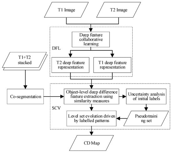
Figure 1.
Flowchart of the proposed change detection (CD) approach.
2.1. Multitemporal Deep Feature Collaborative Learning
The proposed deep feature collaborative learning aims at transforming the multitemporal images into the same high-level feature space to highlight changes and improve the separability between changed and unchanged patterns. SDAE, as its capability of learning robust and abstract representations from the raw data in an unsupervised way, is utilized in the multitemporal deep feature collaborative learning [53,54].
Let us consider two remote sensing images, and of size , acquired in the same geographical area at two different times, and , each having b bands. Both images have been well-preprocessed, including co-registration and radiometric calibration. For each point , we use the point with its spatial neighboring pixels as the input vector, where ω represents the local window size of its neighborhood. The corresponding image patches in the bitemporal images are both vectorized as training samples with dimensions of , as displayed in Figure 2. Then, the feature vectors from the bitemporal images are trained together through a deep feature learning algorithm based on a SDAE model.
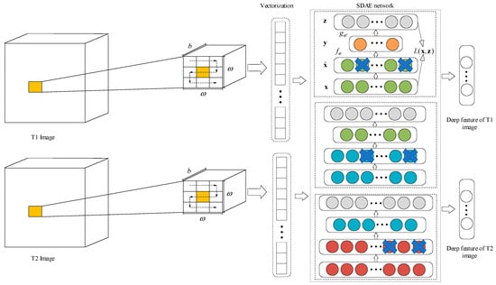
Figure 2.
Process of deep feature collaborative learning of multitemporal images.
An autoencoder is a multi-layer neural network that is used to reconstruct the original input and learn the features. DAE introduces a denoising criterion into the basic autoencoder to make the autoencoder robust to unfavorable noises, and the original inputs are contaminated explicitly by adding random noises during the training. After training, a clean “repaired” input will be reconstructed from the corrupted one and the output values will be as close as the original uncontaminated values [51,55]. This is done by corrupting the original input to get a partially contaminated version , according to a stochastic mapping . Corrupted input is then transformed into a hidden representation through a deterministic mapping :
where the parameter is set to , is the activation function, is a bias vector of dimensionality and is a weight matrix. The activation function is set to the sigmoid function in this paper, i.e.,.
Then we reconstruct a d-dimensional vector through mapping the hidden representation back to the input space. This mapping is an affine mapping, optionally followed by a squashing non-linearity:
parameterized by , where is a bias vector of the dimensionality d and is a weight matrix.
The parameters of the DAE model are optimized in an unsupervised way by minimizing the reconstruction error amounts between a clean and its reconstruction , that is, carrying the following optimization:
where L is the squared error function . The sample size is equal to . After training, the reconstruction layer is removed, and the values of the hidden layer can be used as the representation of input features in a new feature space [51,55].
By stacking multiple DAEs in a hierarchical manner such that the values of hidden layers become the input to the next upper DAE, a SDAE model can be constructed. The SDAE is learnt in a greedy layer-wise fashion using a gradient descent [51,55]. After training the (k-1)th DAE, its learnt representation is used as input to train the kth DAE to learn the next-level representation [54,56]. Then the procedure can be repeated until all the DAEs are trained and the highest-level output representation can be obtained. In this paper, parameters of SDAE are initialized at random and then optimized by stochastic gradient descent. The multitemporal deep features are learned collaboratively in the same high-level feature space based on a SDAE model, as illustrated in Figure 2, thus the multitemporal deep features can be compared directly.
2.2. Deep Difference Feature Extraction
In the proposed CD framework, the co-segmentation using the fractal net evolution approach (FNEA) is applied directly to the stacked bitemporal images to create spatially corresponding objects. FNEA is a region growing algorithm based on a minimum heterogeneity criteria and builds a multi-scale hierarchical structure by merging the neighboring image objects [57,58]. The segment parameters for the FNEA-based segmentation are adjusted and determined with the aid of the ESP tool in this paper.
The deep difference feature map Q is then generated by applying the cosine similarity measure on the multitemporal deep features, as follows:
where is the deep difference feature of the kth object in region . denotes the number of pixels in the kth object. and represent the deep feature vectors of image and , respectively. means the cosine similarity of the two vectors denoted as follows:
2.3. Uncertainty Analysis
In CD problems, it is difficult to obtain reliable supervised information without available ground truth. In this study, we propose to exploit the changed and unchanged patterns by an uncertainty analysis of object labels. The FCM algorithm can obtain more useful information such as the fuzzy membership grade compared to the traditional hard clustering methods [59,60], thus it is adopted to initially cluster the objects in this research. It is an unsupervised method that can classify the deep difference features of the objects into fuzzy clusters. The objective function of the initial clustering algorithm for the deep difference features is represented as the following equation:
where is the deep difference feature vector of the kth object, is the cluster center in the jth cluster, indicates the fuzzy membership grade of associated with the jth cluster, is the squared distance between the feature vector and the cluster .
Based on the initial clustering by FCM, the label uncertainty of each object can be measured by information entropy. Then the pseudo-training set identified as seed patterns can be obtained by selectively thresholding the uncertainty values and comparing between the changed and unchanged fuzzy membership grade, as demonstrated below:
where is the initial label uncertainty of the kth object, denotes a threshold of uncertainty to determine the range of the nearly certain patterns, and contain the changed and unchanged patterns, respectively. As objects with high uncertainty are more likely to be confused with changed and unchanged classes, we can define a relatively small certain region to guarantee the chosen objects contained in the sets and can be accurately labeled with a high probability. Consequently, a pseudo-training set containing relatively reliable samples can be obtained from the deep difference feature map by using the represented rules. The pseudo-training set is made up of the pairs: the changed samples and the unchanged ones , to be used as seed patterns, i.e., and .
2.4. SCV Model
The proposed SCV model aims at finding an optimal contour, which splits the deep difference feature map into non-overlapping regions associated with changed and unchanged classes. In this paper, the pseudo-training information containing labeled patterns is introduced into the traditional CV model. For the given deep difference feature map Q, the proposed energy functional takes on the following form:
where is the proposed energy functional, is the global energy term derived from the CV model and is the incorporated supervised term integrated with the labeled patterns. is the level set function. is the Heaviside step function, i.e., if , and if otherwise. and approximate the change intensities inside and outside the contour, respectively. The typically used regularization term based on the mean curvature in the CV model is eliminated in the proposed model to reduce the computational complexity and constrain the curves towards the object boundaries in the feature map.
Keeping fixed and minimizing the energy , we solve and , as follows:
The energy functional is minimized with respect to by deducing the associated Euler–Lagrange equation for when and remain fixed. Then the new variational formulation for level set evolution can be represented as follows:
where the regularized versions of Heaviside step function and the Dirac delta function are selected as follows:
where is a small number.
The implementation of the proposed algorithm is presented in Table 1.

Table 1.
Pseudocode of the proposed semi-supervised Chan–Vese (SCV) model.
3. Experiments and Analysis
3.1. Datasets
To verify the advantages of the proposed CD approach, four high-resolution multitemporal remote sensing datasets acquired by different platforms and sensors, namely, QuickBird, GF 1, SPOT 5, and Aerial, were considered in the experiments.
The first data set consists of two images of size 598 × 497 pixels, acquired by the QuickBird satellite covering the Xinzhou district in the city of Wuhan, China, in April 2002 and July 2009, with the same spatial resolution of 2.4 m, as shown in Figure 3a.

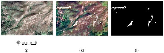
Figure 3.
Data sets used in the experiments: (a)–(c) QuickBird data set acquired in (a) and (b), (c) ground truth map; (d)–(f) GF 1 data set acquired in (d) and (e), (f) ground truth map; (g)–(i) SPOT 5 data set acquired in (g) and (h), (i) ground truth map; (j)–(l) Aerial data set acquired in (j) and (k), (l) ground truth map.
The second data set represented two 2 m high-resolution images acquired by the GF 1 satellite over the Caidian district in Wuhan, China, in April 2016 and August 2018. The images were generated by fusing panchromatic and multispectral images. An area with 800 × 1050 pixels was cropped from the entire images, as displayed in Figure 3b.
The third data set was acquired by the SPOT 5 satellite covering the Wuqing district in the city of Tianjin, China, in April 2008 and February 2009. The size of the dataset is 450 × 400 pixels with a spatial resolution of 2.5 m, as shown in Figure 3c.
The fourth data set contains a pair of bitemporal aerial orthophotos on the Lantau Island, Hong Kong, China. The orthophotos were acquired by Zeiss RMK TOP Aerial Survey Camera System in December 2005 and November 2008, respectively. The images have the size of 743 × 1107 pixels, with a spatial resolution of 0.5 m, as presented in Figure 3d.
Before applying the proposed CD approach, the preprocessing of multitemporal images, including image co-registration and radiometric correction, was performed on the four data sets by ENVI software. The ground truth maps were produced by visual interpretation using ArcGIS software.
3.2. Evaluation Criteria and Experimental Settings
In the experiments, five unsupervised CD methods are selected as the comparison algorithms to verify the advantages of the proposed CD approach, including the classic PCA-K-Means method [17], multi-scale superpixel and deep neural networks (MSDNN) for CD [61], region-based level set evolution (RLSE) method [26], multi-scale object histogram distance (MOHD) method [57], and the object-based unsupervised CD based on the SVM method, denoted as object-based SVM (OSVM) [25].
To verify the effectiveness of the proposed approach, the CD results were evaluated by the following four widely used indices: 1) false alarm (FA) rate, 2) missed detection (MD) rate, 3) total error (TE) rate, and 4) Kappa coefficient [62,63,64].
In the experiments, the local window size of the given pixel and the threshold of uncertainty were set for the proposed approach. The multitemporal deep feature collaborative learning adopted a 3-layer SDAE with structure 27-15-5-2 stacked by three DAEs. Furthermore, we set and for PCA-K-Means, , for MSDNN, and for RLSE, scale = 40, compactness = 0.8, shape = 0.9 for MOHD and , for OSVM in which the Gaussian radial basis function kernel was set for the SVM kernel model. The deep feature learning was implemented in the Python programming language using TensorFlow 1.13.1 (GPU version) on a workstation with an Intel Core i7 CPU and NVIDIA GeForce GTX 1070. The SCV model was implemented in MATLAB R2016a on the workstation.
3.3. Experimental Analysis
The CD maps obtained from the proposed approach and the comparison algorithms on the four datasets are shown in Figure 4, Figure 5, Figure 6 and Figure 7, respectively. From the qualitative point of view, change maps generated with PCA-K-Means display significant noise both in the changed and unchanged regions. Although the homogenous changes can be well-detected by MSDNN, MOHD, and OSVM, many noise spots still exist in the change maps. RLSE uses a thresholding method and morphology operations to reduce errors, but it produces change maps losing a large number of details in the changed regions. By contrast, the proposed approach significantly reduces noise spots and simultaneously retains detailed changes in the change maps.
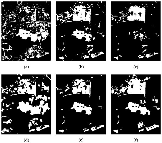
Figure 4.
CD results of QuickBird data set by: (a) PCA-K-Means, (b) MSDNN, (c) RLSE, (d) MOHD, (e) OSVM, and (f) the proposed approach.
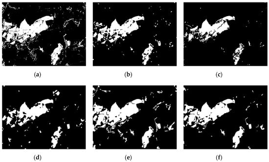
Figure 5.
CD results of GF 1 data set by: (a) PCA-K-Means, (b) MSDNN, (c) RLSE, (d) MOHD, (e) OSVM, and (f) the proposed approach.
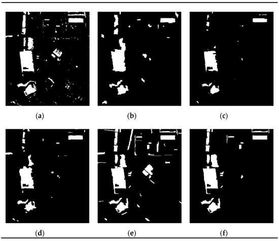
Figure 6.
CD results of SPOT 5 data set by: (a) PCA-K-Means, (b) MSDNN, (c) RLSE, (d) MOHD, (e) OSVM, and (f) the proposed approach.
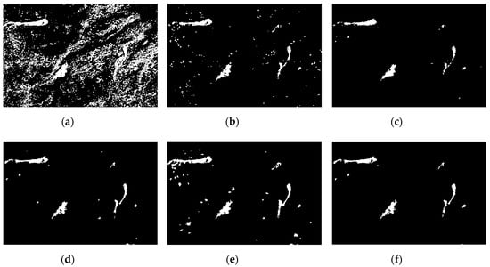
Figure 7.
CD results of Aerial data set by: (a) PCA-K-Means, (b) MSDNN, (c) RLSE, (d) MOHD, (e) OSVM, and (f) the proposed approach.
Deep difference feature maps and uncertainty analysis results of the four test data sets are given in Figure 8. As can be seen, the deep difference feature maps can highlight change intensities of objects. In addition, the changed and unchanged samples identified as seed patterns can be obtained from deep difference feature maps through uncertainty analysis
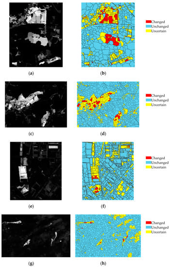
Figure 8.
Deep difference feature maps and uncertainty analysis results: (a)–(b) QuickBird data set; (c)–(d) GF 1 data set; (e)–(f) SPOT 5 data set; (g)–(h) Aerial data set.
Figure 9 represents the evolution process of the level set function from the initial contour to the final result in the SCV model compared to the traditional CV model. The initial curves were circles evenly covering the entire deep difference feature map. As shown in Figure 8, the SCV model has the capability of causing the level curves to rapidly evolve towards the object boundaries compared to the CV model.
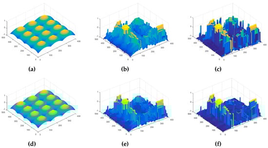
Figure 9.
Level set evolution of the proposed SCV model compared to the CV model in terms of SPOT 5 data: (a) initialization of CV; (b) iteration 20 of CV; (c) iteration 200 of CV (final contour); (d) initialization of SCV; (e) iteration 20 of SCV; (f) iteration 30 of SCV (final contour).
Table 2, Table 3, Table 4 and Table 5 illustrate the quantitative error measures obtained by all the CD methods used in this research. From the point of view of KC and TE rates, the proposed approach clearly exceeds the other five methods, which indicates that the proposed approach achieves the most accurate CD results compared to the ground truths. In terms of QuickBird data, although the proposed approach generates more FAs than RLSE and OSVM, the MD rate has been significantly reduced by the proposed approach. Consequently, the proposed approach generates the least amount of TEs. The similar performance can be found in results of GF 1 data and SPOT 5 data. RLSE generates the least FAs, but the largest amount of MD rates. However, the proposed approach is capable of extracting more complete changed areas. As a result, the proposed approach produces the lowest TEs. With respect to the aerial data, the PCA-K-Means and OSVM achieve lower MD rates and larger FA rates. In comparison, the proposed approach performs significantly better in terms of TEs and FAs. Overall, the proposed approach has demonstrated competitive advantages over the compared methods throughout the experiments.
Table 2.
Accuracy comparison among different methods on the QuickBird data set.
Table 3.
Accuracy comparison among different methods on the GF 1 data set.
Table 4.
Accuracy comparison among different methods on the SPOT 5 data set.
Table 5.
Accuracy comparison among different methods on the Aerial data set.
To test the impact of the network structure of SDAE in our deep feature learning model, different network structures have been taken into consideration to evaluate their influences over the accuracy of the CD results. Figure 10 illustrates the variations in the TE rates and KC values with CD results obtained by SDAE with different structures, in which SDAE-2 is a 2-layer SDAE with structure 27-15-2 stacked by two DAEs, SDAE-3 is a 3-layer SDAE with structure 27-15-5-2 stacked by three DAEs, SDAE-4 is a 4-layer SDAE with structure 27-20-15-5-2 stacked by four DAEs, and SDAE-5 is a 5-layer SDAE with structure 27-20-15-10-5-2 stacked by five DAEs.
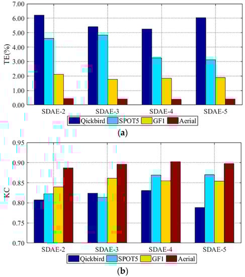
Figure 10.
Variations in: (a) TE rates and (b) KC of the proposed approach when different change maps were obtained by SDAE with different network structures for the test data sets.
In general, a deeper network can learn more useful abstract features from the input data. The CD results in this paper are related to both deep difference features and the SCV model. For the SPOT 5 and Aerial data sets, the deeper network such as SDAE-3, SDAE-4, and SDAE-5 can generate more accurate results than SDAE-2, and the TE and KC values obtained by SDAE-3, SDAE-4, and SDAE-5 are close. Similarly, for the GF 1 data set, the SDAE-4 and SDAE-5 with deeper network structures can obtain more accurate results than SDAE-2 and SDAE-3. Nevertheless, for the QuickBird data set, the SDAE-5 stacked by five DAEs undergoes a decline in accuracy because some detailed changes are lacking in the CD result.
In the SCV model, the T values determine the uncertainty of pseudo-training samples and the reliability of the labeled patterns. The variations in the TE rates and KC with different T values in Equation (9) of the SCV model are displayed in Figure 11. Different change maps produced by T values ranging from 0.1 to 0.9 with a step of 0.1 are used to analyze the effects of different T values on CD results. In general, the TE rates rise with the increase of the value of T and the KC values undergo a decline. It indicates that the more reliable pseudo-training samples with smaller T values can generate more accurate CD results. Labeled patterns obtained by larger T values may guide the level curves to the unexpected objects boundaries and result in a decrease of the accuracy of CD maps, especially for Aerial data.

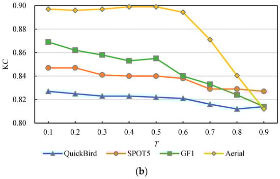
Figure 11.
Variations in: (a) TE rates and (b) KC of the proposed approach when different change maps were obtained by T values ranging from 0.1 to 0.9, with a step of 0.1 for the test data sets.
4. Discussion
The experimental results on four remote sensing data sets from different sensors have corroborated the proposed CD approach is superior to other methods through the qualitative and quantitative analysis. In the multitemporal deep feature collaborative learning, the deeper network can generate more abstract difference features, but the loss of detailed changes may occur in the deep feature map when there are too much layers in the deep networks. Reliable labeled patterns for the SCV model can be obtained by smaller T values and guide the level curves to the changed object boundaries.
The proposed CD approach in this research is mainly based on comparing images at two different times–the bitemporal approach, but it can also be used for CD with more than two images. For example, the image-objects can be generated by segmenting the multi-temporal images together and the multitemporal deep feature collaborative learning can use multi-temporal images as input. The experimental results have confirmed the robustness of the proposed approach and its ability of handling different land cover change types, such as urban sprawl (QuickBird data, GF1 data, and SPOT5 data), vegetation restoration (QuickBird data), and disaster monitoring (Aerial data). This research focuses on automatically and efficiently detecting land cover changes from remote sensing images. It provides a solution for CD without high-quality samples or prior knowledge. To further improve the reliability of CD results, the additional information can be used in the specific CD applications, such as analyzing historical data and other supplementary data to obtain the driving factor of land cover changes and integrating the slope and aspect information in the landslide mapping.
5. Conclusions
This paper has presented a novel approach for CD from multitemporal high-resolution remote sensing images without any prior information. The multitemporal deep feature collaborative learning based on SDAE is developed to obtain the deep feature representations of multitemporal images. Then, the object-level abstract difference features can be obtained through multitemporal co-segmentation and the feature similarity measure. After that, a SCV model is used to extract the final changed regions integrated with the labeled patterns derived from an uncertainty analysis.
The experimental results on four data sets acquired by different sensors have corroborated the effectiveness and reliability of the proposed approach for CD. Compared to PCA-K-Means, MSDNN, RLSE, MOHD, and OSVM, the proposed approach performs better through qualitative and quantitative evaluations. The proposed approach can not only reduce the influence of speckle noise, but also retain the detailed changes. Thus, it achieves the most accurate CD results among all the methods in the experiments.
The main advantages of the proposed approach are that deep features of original multitemporal images can be represented in the same high-level feature space through deep feature collaborative learning to effectively exploit the abstract difference features and improve the separability between changed and unchanged patterns. Moreover, the pseudo-training set containing the labeled patterns derived from uncertainty analysis is incorporated into the level set evolution functional to efficiently drive the level curves towards more accurate changed object boundaries.
Further improvement will be considered in modifying this algorithm to handle the CD problems when the multitemporal images come from different sensors and when detecting the multi-class changes from the images.
Author Contributions
X.Z. and W.S. were responsible for the overall design of the study. X.Z. performed the experiments and drafted the manuscript, which was revised by all authors. X.Z., Z.L., and F.P. carried out the data processing. All authors read and approved the final manuscript.
Funding
This research was funded by the National Natural Science Foundation of China under grants 41801323, 41701511.
Acknowledgments
The authors are grateful to the editors and referees for their constructive criticism on this paper.
Conflicts of Interest
The authors declare no conflict of interest.
References
- Hansen, M.C.; Loveland, T.R. A review of large area monitoring of land cover change using Landsat data. Remote Sens. Environ. 2012, 122, 66–74. [Google Scholar] [CrossRef]
- Stramondo, S.; Bignami, C.; Chini, M.; Pierdicca, N.; Tertulliani, A. Satellite radar and optical remote sensing for earthquake damage detection: Results from different case studies. Int. J. Remote Sens. 2006, 27, 4433–4447. [Google Scholar] [CrossRef]
- Foley, J.A.; DeFries, R.; Asner, G.P.; Barford, C.; Bonan, G.; Carpenter, S.R.; Chapin, F.S.; Coe, M.T.; Daily, G.C.; Gibbs, H.K. Global consequences of land use. Science 2005, 309, 570–574. [Google Scholar] [CrossRef]
- Coppin, P.; Jonckheere, I.; Nackaerts, K.; Muys, B.; Lambin, E. Review ArticleDigital change detection methods in ecosystem monitoring: A review. Int. J. Remote Sens. 2004, 25, 1565–1596. [Google Scholar] [CrossRef]
- Lu, D.; Mausel, P.; Brondizio, E.; Moran, E. Change detection techniques. Int. J. Remote Sens. 2004, 25, 2365–2401. [Google Scholar] [CrossRef]
- Tewkesbury, A.P.; Comber, A.J.; Tate, N.J.; Lamb, A.; Fisher, P.F. A critical synthesis of remotely sensed optical image change detection techniques. Remote Sens. Environ. 2015, 160, 1–14. [Google Scholar] [CrossRef]
- Lv, Z.Y.; Liu, T.F.; Zhang, P.; Benediktsson, J.A.; Lei, T.; Zhang, X. Novel Adaptive Histogram Trend Similarity Approach for Land Cover Change Detection by Using Bitemporal Very-High-Resolution Remote Sensing Images. IEEE Trans. Geosci. Remote Sens. 2019, 57, 9554–9574. [Google Scholar] [CrossRef]
- Saha, S.; Bovolo, F.; Bruzzone, L. Unsupervised Deep Change Vector Analysis for Multiple-Change Detection in VHR Images. IEEE Trans. Geosci. Remote Sens. 2019, 57, 3677–3693. [Google Scholar] [CrossRef]
- Zhan, Y.; Fu, K.; Yan, M.; Sun, X.; Wang, H.; Qiu, X. Change Detection Based on Deep Siamese Convolutional Network for Optical Aerial Images. IEEE Geosci. Remote Sens. Lett. 2017, 14, 1845–1849. [Google Scholar] [CrossRef]
- Hussain, M.; Chen, D.; Cheng, A.; Wei, H.; Stanley, D. Change detection from remotely sensed images: From pixel-based to object-based approaches. ISPRS J. Photogramm. Remote Sens. 2013, 80, 91–106. [Google Scholar] [CrossRef]
- Blaschke, T.; Hay, G.J.; Weng, Q.; Resch, B. Collective Sensing: Integrating Geospatial Technologies to Understand Urban Systems—An Overview. Remote Sens. 2011, 3, 1743–1776. [Google Scholar] [CrossRef]
- Im, J.; Rhee, J.; Jensen, J.R.; Hodgson, M.E. An automated binary change detection model using a calibration approach. Remote Sens. Environ. 2007, 106, 89–105. [Google Scholar] [CrossRef]
- Serra, P.; Pons, X.; Sauri, D. Post-classification change detection with data from different sensors: Some accuracy considerations. Int. J. Remote Sens. 2003, 24, 3311–3340. [Google Scholar] [CrossRef]
- Bruzzone, L.; Prieto, D. Automatic analysis of the difference image for unsupervised change detection. IEEE Trans. Geosci. Remote Sens. 2000, 38, 1171–1182. [Google Scholar] [CrossRef]
- Zhang, X.; Shi, W.; Hao, M.; Shao, P.; Lyu, X. Level set incorporated with an improved MRF model for unsupervised change detection for satellite images. Eur. J. Remote Sens. 2017, 50, 202–210. [Google Scholar] [CrossRef]
- Lv, Z.; Liu, T.; Wan, Y.; Benediktsson, J.A.; Zhang, X. Post-Processing Approach for Refining Raw Land Cover Change Detection of Very High-Resolution Remote Sensing Images. Remote Sens. 2018, 10, 472. [Google Scholar] [CrossRef]
- Celik, T. Unsupervised Change Detection in Satellite Images Using Principal Component Analysis and k-Means Clustering. IEEE Geosci. Remote Sens. Lett. 2009, 6, 772–776. [Google Scholar] [CrossRef]
- Zhang, Y.; Peng, D.; Huang, X. Object-Based Change Detection for VHR Images Based on Multiscale Uncertainty Analysis. IEEE Geosci. Remote Sens. Lett. 2018, 15, 13–17. [Google Scholar] [CrossRef]
- Leichtle, T.; Geiß, C.; Wurm, M.; Lakes, T.; Taubenböck, H. Unsupervised change detection in VHR remote sensing imagery—An object-based clustering approach in a dynamic urban environment. Int. J. Appl. Earth Obs. Geoinf. 2017, 54, 15–27. [Google Scholar] [CrossRef]
- Ma, L.; Li, M.; Blaschke, T.; Ma, X.; Tiede, D.; Cheng, L.; Chen, Z.; Chen, D. Object-based change detection in urban areas: The effects of segmentation strategy, scale, and feature space on unsupervised methods. Remote Sens. 2016, 8, 761. [Google Scholar] [CrossRef]
- Cai, L.; Shi, W.; Zhang, H.; Hao, M. Object-oriented change detection method based on adaptive multi-method combination for remote-sensing images. Int. J. Remote Sens. 2016, 37, 5457–5471. [Google Scholar] [CrossRef]
- Wang, B.; Choi, S.; Byun, Y.; Lee, S.; Choi, J. Object-Based Change Detection of Very High Resolution Satellite Imagery Using the Cross-Sharpening of Multitemporal Data. IEEE Geosci. Remote Sens. Lett. 2015, 12, 1151–1155. [Google Scholar] [CrossRef]
- Shao, P.; Shi, W.; He, P.; Hao, M.; Zhang, X. Novel Approach to Unsupervised Change Detection Based on a Robust Semi-Supervised FCM Clustering Algorithm. Remote Sens. 2016, 8, 264. [Google Scholar] [CrossRef]
- Ardila, J.P.; Bijker, W.; Tolpekin, V.A.; Stein, A. Multitemporal change detection of urban trees using localized region-based active contours in VHR images. Remote Sens. Environ. 2012, 124, 413–426. [Google Scholar] [CrossRef]
- Cao, G.; Li, Y.; Liu, Y.; Shang, Y. Automatic change detection in high-resolution remote-sensing images by means of level set evolution and support vector machine classification. Int. J. Remote Sens. 2014, 35, 6255–6270. [Google Scholar] [CrossRef]
- Li, Z.; Shi, W.; Myint, S.W.; Lu, P.; Wang, Q. Semi-automated landslide inventory mapping from bitemporal aerial photographs using change detection and level set method. Remote Sens. Environ. 2016, 175, 215–230. [Google Scholar] [CrossRef]
- Zhang, X.; Shi, W.; Liang, P.; Hao, M. Level set evolution with local uncertainty constraints for unsupervised change detection. Remote Sens. Lett. 2017, 8, 811–820. [Google Scholar] [CrossRef]
- Li, H.; Gong, M.; Liu, J. A local statistical fuzzy active contour model for change detection. IEEE Geosci. Remote Sens. Lett. 2015, 12, 582–586. [Google Scholar] [CrossRef]
- Blaschke, T.; Hay, G.J.; Kelly, M.; Lang, S.; Hofmann, P.; Addink, E.; Feitosa, R.Q.; Van Der Meer, F.; Van Der Werff, H.; Van Coillie, F.; et al. Geographic Object-Based Image Analysis—Towards a new paradigm. ISPRS J. Photogramm. Remote Sens. 2014, 87, 180–191. [Google Scholar] [CrossRef]
- Blaschke, T. Object based image analysis for remote sensing. ISPRS J. Photogramm. Remote Sens. 2010, 65, 2–16. [Google Scholar] [CrossRef]
- Lv, Z.Y.; Shi, W.; Zhang, X.; Benediktsson, J.A. Landslide Inventory Mapping From Bitemporal High-Resolution Remote Sensing Images Using Change Detection and Multiscale Segmentation. IEEE J. Sel. Top. Appl. Earth Obs. Remote Sens. 2018, 11, 1520–1532. [Google Scholar] [CrossRef]
- Im, J.; Jensen, J.R.; Tullis, J.A. Object-based change detection using correlation image analysis and image segmentation. Int. J. Remote Sens. 2008, 29, 399–423. [Google Scholar] [CrossRef]
- Volpi, M.; Tuia, D.; Bovolo, F.; Kanevski, M.; Bruzzone, L. Supervised change detection in VHR images using contextual information and support vector machines. Int. J. Appl. Earth Obs. Geoinf. 2013, 20, 77–85. [Google Scholar] [CrossRef]
- Bovolo, F.; Bruzzone, L.; Marconcini, M. A Novel Approach to Unsupervised Change Detection Based on a Semisupervised SVM and a Similarity Measure. IEEE Trans. Geosci. Remote Sens. 2008, 46, 2070–2082. [Google Scholar] [CrossRef]
- Huo, C.; Zhou, Z.; Lu, H.; Pan, C.; Chen, K. Fast Object-Level Change Detection for VHR Images. IEEE Geosci. Remote Sens. Lett. 2009, 7, 118–122. [Google Scholar] [CrossRef]
- Neagoe, V.-E.; Stoica, R.-M.; Ciurea, A.-I.; Bruzzone, L.; Bovolo, F. Concurrent Self-Organizing Maps for Supervised/Unsupervised Change Detection in Remote Sensing Images. IEEE J. Sel. Top. Appl. Earth Obs. Remote Sens. 2014, 7, 3525–3533. [Google Scholar] [CrossRef]
- Ghosh, S.; Roy, M.; Ghosh, A. Semi-supervised change detection using modified self-organizing feature map neural network. Appl. Soft Comput. 2014, 15, 1–20. [Google Scholar] [CrossRef]
- Homer, C.; Dewitz, J.; Yang, L.; Jin, S.; Danielson, P.; Xian, G.; Coulston, J.; Herold, N.; Wickham, J.; Megown, K. Completion of the 2011 National Land Cover Database for the conterminous United States–representing a decade of land cover change information. Photogramm. Eng. Remote Sens. 2015, 81, 345–354. [Google Scholar]
- Im, J.; Jensen, J.R. A change detection model based on neighborhood correlation image analysis and decision tree classification. Remote Sens. Environ. 2005, 99, 326–340. [Google Scholar] [CrossRef]
- Sesnie, S.E.; Gessler, P.E.; Finegan, B.; Thessler, S. Integrating Landsat TM and SRTM-DEM derived variables with decision trees for habitat classification and change detection in complex neotropical environments. Remote Sens. Environ. 2008, 112, 2145–2159. [Google Scholar] [CrossRef]
- Xu, X.; Li, W.; Ran, Q.; Du, Q.; Gao, L.; Zhang, B. Multisource remote sensing data classification based on convolutional neural network. IEEE Trans. Geosci. Remote Sens. 2017, 56, 937–949. [Google Scholar] [CrossRef]
- Wu, H.; Prasad, S. Convolutional Recurrent Neural Networks for Hyperspectral Data Classification. Remote Sens. 2017, 9, 298. [Google Scholar] [CrossRef]
- Zhang, C.; Sargent, I.; Pan, X.; Li, H.; Gardiner, A.; Hare, J.; Atkinson, P.M. An object-based convolutional neural network (OCNN) for urban land use classification. Remote Sens. Environ. 2018, 216, 57–70. [Google Scholar] [CrossRef]
- Lei, T.; Zhang, Y.; Lv, Z.; Li, S.; Liu, S.; Nandi, A.K. Landslide Inventory Mapping from Bitemporal Images Using Deep Convolutional Neural Networks. IEEE Geosci. Remote Sens. Lett. 2019, 16, 982–986. [Google Scholar] [CrossRef]
- Bischke, B.; Helber, P.; Folz, J.; Borth, D.; Dengel, A. Multi-Task Learning for Segmentation of Building Footprints with Deep Neural Networks. In Proceedings of the 2019 IEEE International Conference on Image Processing (ICIP), Taipei, Taiwan, 22–25 September 2019; pp. 1480–1484. [Google Scholar]
- Liu, W.; Cheng, D.; Yin, P.; Yang, M.; Li, E.; Xie, M.; Zhang, L. Small Manhole Cover Detection in Remote Sensing Imagery with Deep Convolutional Neural Networks. ISPRS Int. J. Geo-Inf. 2019, 8, 49. [Google Scholar] [CrossRef]
- Mahdianpari, M.; Salehi, B.; Rezaee, M.; Mohammadimanesh, F.; Zhang, Y. Very Deep Convolutional Neural Networks for Complex Land Cover Mapping Using Multispectral Remote Sensing Imagery. Remote Sens. 2018, 10, 1119. [Google Scholar] [CrossRef]
- Khan, S.H.; He, X.; Porikli, F.; Bennamoun, M. Forest Change Detection in Incomplete Satellite Images with Deep Neural Networks. IEEE Trans. Geosci. Remote Sens. 2017, 55, 5407–5423. [Google Scholar] [CrossRef]
- Mou, L.; Bruzzone, L.; Zhu, X.X. Learning Spectral-Spatial-Temporal Features via a Recurrent Convolutional Neural Network for Change Detection in Multispectral Imagery. IEEE Trans. Geosci. Remote Sens. 2018, 57, 924–935. [Google Scholar] [CrossRef]
- Wang, Q.; Yuan, Z.; Du, Q.; Li, X. GETNET: A General End-to-End 2-D CNN Framework for Hyperspectral Image Change Detection. IEEE Trans. Geosci. Remote Sens. 2018, 57, 3–13. [Google Scholar] [CrossRef]
- Zhang, P.; Gong, M.; Su, L.; Liu, J.; Li, Z. Change detection based on deep feature representation and mapping transformation for multi-spatial-resolution remote sensing images. ISPRS J. Photogramm. Remote Sens. 2016, 116, 24–41. [Google Scholar] [CrossRef]
- Gong, M.; Zhan, T.; Zhang, P.; Miao, Q. Superpixel-Based Difference Representation Learning for Change Detection in Multispectral Remote Sensing Images. IEEE Trans. Geosci. Remote Sens. 2017, 55, 2658–2673. [Google Scholar] [CrossRef]
- Xie, J.; Xu, L.; Chen, E. Image denoising and inpainting with deep neural networks. In Proceedings of the Advances in Neural Information Processing Systems, Lake Tahoe, NV, USA, 3–6 December 2012; pp. 341–349. [Google Scholar]
- Vincent, P.; Larochelle, H.; Lajoie, I.; Bengio, Y.; Manzagol, P.-A. Stacked denoising autoencoders: Learning useful representations in a deep network with a local denoising criterion. J. Mach. Learn. Res. 2010, 11, 3371–3408. [Google Scholar]
- Zhang, X.; Chen, G.; Wang, W.; Wang, Q.; Dai, F. Object-Based Land-Cover Supervised Classification for Very-High-Resolution UAV Images Using Stacked Denoising Autoencoders. IEEE J. Sel. Top. Appl. Earth Obs. Remote Sens. 2017, 10, 3373–3385. [Google Scholar] [CrossRef]
- Vincent, P.; LaRochelle, H.; Bengio, Y.; Manzagol, P.-A. Extracting and composing robust features with denoising autoencoders. In Proceedings of the 25th International Conference on Machine Learning, Helsinki, Finland, 5–9 July 2008; pp. 1096–1103. [Google Scholar]
- Lv, Z.; Liu, T.; Benediktsson, J.A.; Lei, T.; Wan, Y. Multi-Scale Object Histogram Distance for LCCD Using Bi-Temporal Very-High-Resolution Remote Sensing Images. Remote Sens. 2018, 10, 1809. [Google Scholar] [CrossRef]
- Gu, H.; Han, Y.; Yang, Y.; Li, H.; Liu, Z.; Soergel, U.; Blaschke, T.; Cui, S. An Efficient Parallel Multi-Scale Segmentation Method for Remote Sensing Imagery. Remote Sens. 2018, 10, 590. [Google Scholar] [CrossRef]
- Lei, T.; Jia, X.; Zhang, Y.; He, L.; Meng, H.; Nandi, A.K. Significantly Fast and Robust Fuzzy C-Means Clustering Algorithm Based on Morphological Reconstruction and Membership Filtering. IEEE Trans. Fuzzy Syst. 2018, 26, 3027–3041. [Google Scholar] [CrossRef]
- Lei, T.; Xue, D.; Lv, Z.; Li, S.; Zhang, Y.; Nandi, A.K. Unsupervised change detection using fast fuzzy clustering for landslide mapping from very high-resolution images. Remote Sens. 2018, 10, 1381. [Google Scholar] [CrossRef]
- Lei, Y.; Liu, X.; Shi, J.; Lei, C.; Wang, J. Multiscale superpixel segmentation with deep features for change detection. IEEE Access 2019, 7, 36600–36616. [Google Scholar] [CrossRef]
- Yetgin, Z. Unsupervised change detection of satellite images using local gradual descent. IEEE Trans. Geosci. Remote Sens. 2012, 50, 1919–1929. [Google Scholar] [CrossRef]
- Shi, W.; Zhang, X.; Hao, M.; Shao, P.; Cai, L.; Lyu, X. Validation of land cover products using reliability evaluation methods. Remote Sens. 2015, 7, 7846–7864. [Google Scholar] [CrossRef]
- Zhang, X.; Shi, W.; Lv, Z. Uncertainty Assessment in Multitemporal Land Use/Cover Mapping with Classification System Semantic Heterogeneity. Remote Sens. 2019, 11, 2509. [Google Scholar] [CrossRef]
© 2019 by the authors. Licensee MDPI, Basel, Switzerland. This article is an open access article distributed under the terms and conditions of the Creative Commons Attribution (CC BY) license (http://creativecommons.org/licenses/by/4.0/).