1. Introduction
Tree species classification is a challenging and important task for large-area monitoring and managing of forests. For many applications, it is an important step to first retrieve the tree species in order to enable the detection of specific traits such as nutrition state, water content, various stresses, diseases, and other relevant parameters in a species-specific context.
In 2015, Fraunhofer IFF conducted measurement flights over forests in Saxony Anhalt and Thuringia, Germany for two reasons: (1) to develop new methods for detection of biotic stresses related to oak feeding society (green oak-leaf roller,
Tortrix viridana), mottled umber (
Erannis defoliaria), and winter moth (
Operophthera brumata); and (2) to support ground-based forest inventory by airborne assessment of tree species and tree vitality. Both require reliable detection of oak trees as well as other tree species in mixed forests. Hyperspectral imaging was chosen as a means to address these challenging tasks. It is an emerging measurement technique frequently used for optical non-invasive characterization of surfaces and materials. In contrast to the analysis of conventional digital images, multiple image channels that correspond to reflected or transmitted light of a certain small wavelength range, must be taken into account. A typical hyperspectral image consists of hundreds of image bands. A good introduction to hyperspectral image classification was provided by Bioucas-Dias et al. [
1]. Challenges mentioned are the limited number of labeled samples and the need to combine spectral and spatial information to obtain good results. Typically, the high-dimensional nature of the data and strong correlations among spectral bands require the extraction of suitable features prior to training of a classifier. The authors also highlight the importance of high spatial image resolution, as most classification techniques assume a single predominant spectral signature per pixel. In contrast, a low image resolution leads to mixed pixels, which requires spectral unmixing as an additional preprocessing step [
2].
Wang et al. [
3] dedicated a chapter of their book “Remote Sensing of Natural Resources” to the classification of tree species. They listed principal component analysis (PCA), minimum noisef fraction (MNF), canonical discriminant analysis, partial least squares regression (PLS), and wavelet transform as common feature extraction methods. They also provide references where these techniques have been applied. Moreover, an overview on the application of classifiers containing support vector machines (SVM), classification and regression trees (CART), and artificial neural networks (ANN) is given. Fassnacht et al. [
4] published a recent survey on tree species classification. The authors considered different types of discriminant analysis (linear, quadratic, canonical, stepwise, regularized, and penalized), SVM, random forest, and maximum likelihood classifiers. With reference to experiences from previous work (e.g., [
5]), the authors draw the conclusion that the choice of the classifier is less important than adequate data preprocessing to obtain good results.
Féret et al. [
6] investigated the discrimination of 17 tree species in tropical forests. A comparison of different parametric and non-parametric methods showed that SVM with linear or radial basis function kernels outperformed other classifiers given a large number of training samples. For smaller training sets, the authors recommend regularized discriminant analysis. Richter et al. [
7] introduced a modified version of discriminant analysis based on PLS. The authors compared their approach to random forests and SVMs on an airborne hyperspectral dataset recorded over a German forest area and obtained better results compared to these classifiers. In this study, random forests performed notably worse than SVMs. To a smaller extent, this is also the result of studies in the Southern Alps conducted by Dalponte et al. [
8]. The authors show that the overall accuracy of tree species identification increased by the integration of LiDAR data in addition to hyperspectral measurements.
Xia et al. [
9] have demonstrated successful usage of an ensemble classifier on hyperspectral benchmark datasets. In addition, the concept of rotation forests, originally introduced by Rodriguez et al. [
10], was successfully applied using CARTs as base classifiers. Compared to MNF, independent component analysis (ICA), and local Fisher discriminant analysis (LFDA) as transformation approaches, the choice of PCA yields the highest accuracy in their studies.
Instead of searching for a favorable transformation of the feature space, certain spectral bands can be selected based on close correspondence to biochemical traits and physical properties of the observed plants. This concept led to a variety of general or trait-specific vegetation indices. Lausch et al. [
11] list spectral indices related to greenness and other vitality parameters, mainly using bands in the spectral range of 450–890 nm. A similar overview can be found in a disease detection report published by Sankaran et al. [
12]. Mutanga et al. [
13] investigated the relationship between water content and spectral variables. Besides known water absorption features located at three different bands, related spectral indices (NDWI [
14], WI [
15]) and continuum-removed features were included in their correlation analysis.
Airborne hyperspectral imaging generates a large amount of data of which usually only a small fraction is labeled with reference data. Therefore, semi-supervised approaches for classifier training aim to make use of unlabeled data for hyperspectral image classification as well. Here, the term semi-supervised is used for all approaches that includes both labeled and unlabeled data in the training of classifiers to enhance the classification performance. It emphasizes the fact that reference data is still required, but a much larger dataset contributes to the final classifier.
Ayerdi et al. [
16] describe a data augmentation method as a means to use the information of unlabeled data. After performing a clustering in the spectral domain, labeled pixels propagate their label to neighboring unlabeled pixels in the spatial domain if they belong to the same cluster.
Wenzhi et al. [
17] introduce a semi-supervised feature extraction algorithm named semi-supervised local discriminant analysis (SELD). The combination of an unsupervised local linear feature extraction method with linear discriminant analysis (LDA) results in a projection that separates the different classes while preserving local neighborhoods. In their evaluation, SELD is compared to different feature extraction methods such as PCA and LDA and obtained the best results on several datasets with different classifiers.
Since SVMs are reported to perform well on hyperspectral datasets, an extension to the semi-supervised case is desirable. Vapnik et al. [
18] proposed the idea of transductive SVMs, which was applied to hyperspectral data later on (e.g., by Bruzzone et al. [
19]).
It is common practice to use both spectral and spatial information for classification. For the problem of tree species classification, a popular approach is to identify individual tree crowns (ITCs), before starting the classification process. Féret et al. [
6] used mean shift clustering to segment ITCs and evaluated two different classification methods: object-based classification of the mean spectrum per ITC and majority class assignment based on the decisions per pixel within the ITC. The authors report an increased accuracy for both approaches compared to pixelwise classification without prior tree crown segmentation. Dalponte et al. [
20] incorporated the assumption that all pixels belonging to an ITC should have the same label within the training process of a semi-supervised SVM. An improvement over conventional SVMs was observed, especially if the number of training samples is small. The problems related to small numbers of training samples can also be effectively addressed by tensor-based linear and non-linear models as proposed by Makantasis et al. in [
21].
Ghamisi et al. [
22] proposed a spectral-spatial classifier based on hidden Markov random fields and SVMs. This fully automatic approach performed better than SVMs on widely used datasets. Li et al. [
23] integrate spectral and spatial information in a robust Bayesian framework, addressing problems related to noise, the presence of mixed pixels, and small number of training samples. The authors evaluated their algorithm along with several state-of-the-art methods and achieved notably better results in terms of accuracy. Zhang et al. [
24] introduced a sparse ensemble learning method, which allows for information sharing between neighboring pixels during the optimization process. While any classifier can potentially be used, the experiments in this study used CARTs. The authors report not only better accuracy, but also a lower runtime of the trained ensemble compared to traditional ensemble methods.
Since the extraction of handcrafted features is time consuming and complex, Makantasis et al. [
25] suggest a convolutional neural network (CNN) to automatically construct high-level features. The dimensionality of the input data is reduced by a PCA first and then three convolutional layers hierarchically detect features, which are classified by two fully connected layers in the end. The CNN outperformed different types of SVMs on benchmark datasets.
Ayerdi et al. [
16] suggested a regularization step after classification: each pixel adapts its label to the majority class in its neighborhood. If rather homogeneous tree species distributions in the area under consideration can be assumed, this technique leads to more plausible results.
The review of the literature shows a number of promising approaches to classify tree species from hyperspectral imaging data. It was especially shown that recent advances in image classification with CNNs are transferable to hyperspectral image classification. However, for any new application and dataset, several state-of-the-art classifiers and different feature spaces in question must be tested to prove the suitability and superiority of an approach [
26]. Given this requirement, the question arises: what benefits the combination of the best available classification techniques and turns them into an ensemble classifier capable of providing for the problem of tree species classification? To answer this question, we focus on popular voting strategies, which are easy to apply to any group of classifiers.
2. Materials and Methods
2.1. Datasets
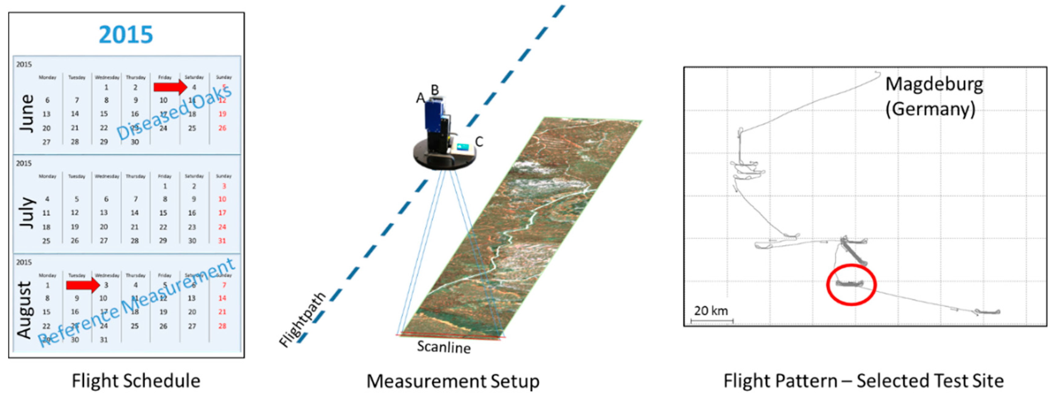
Figure 1 illustrates the acquisition of the datasets. Hyperspectral imaging data has been recorded during two measurement flights over forests in Saxony Anhalt and Thuringia (Germany) to determine tree species and investigate oak tree specific biotic stresses. Used cameras were NEO Hyspex VNIR 1600 and NEO Hyspex SWIR 320m-e. Cameras and inertial measurement unit (IMU) Novatel SPAN CPT were fixed on a stabilized mount (see
Figure 1). The recording of the flight path and orientation of the line scanning camera systems by the IMU is crucial for later alignment of the scanlines into an image. Experiments reported here are based on Hyspex VNIR 1600 images recorded during the second flight. The reasons are to minimize potential errors from alignment and interpolation of the low resolution Hyspex SWIR 320m-e camera to match the grid of the VNIR camera, better weather conditions during the second flight (no cloud cover), and the recovery of diseased oak trees after secondary ‘lammas’ shoots [
27], which is expected to ease tree species classification.
Orthorectification of the line scanning data was done with parametric geocoding using the software PARGE [
28]. Radiometric corrections were performed with the software ATCOR-4 [
29].
One of the major challenges while classifying tree species is the availability of training data that represents differences between individual trees of one species, differences between development stages of individual trees as well as the differences between tree species. In order to account for the variability and to minimize the necessary fieldwork, existing databases and high-resolution aerial images were used to determine areas with a single dominant tree species.
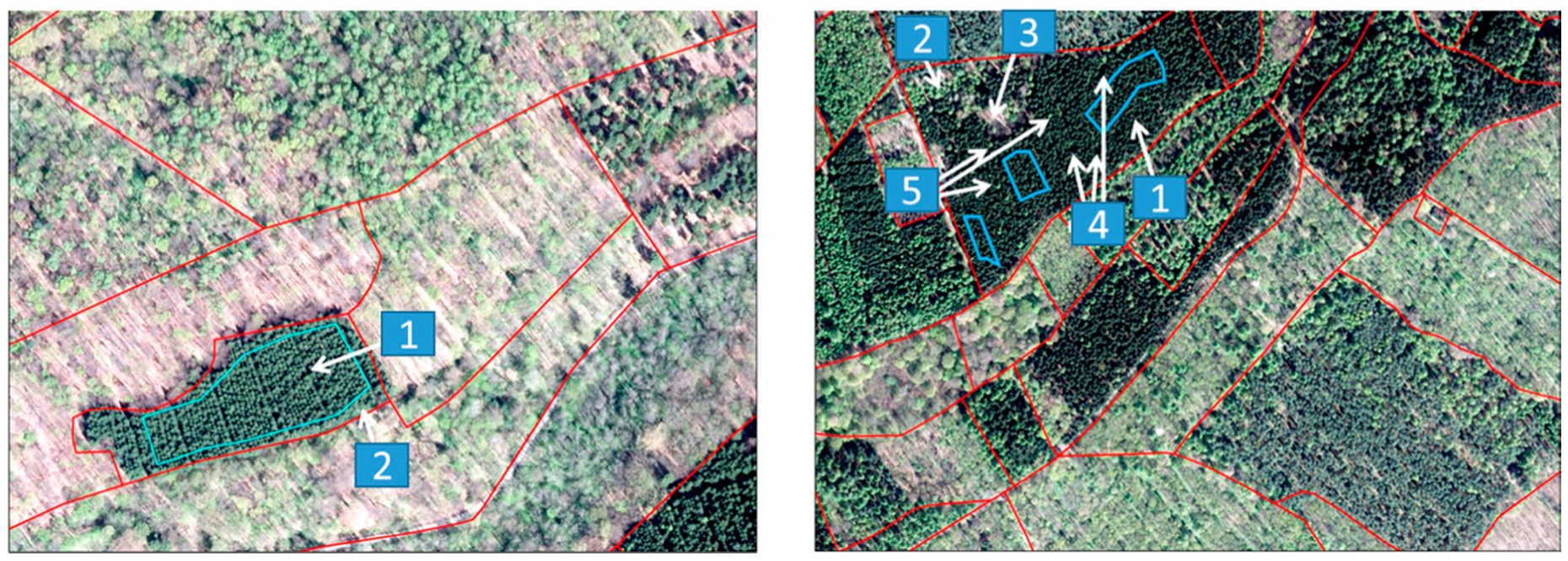
Figure 2 illustrates the results of the selection process. As shown, potential error sources such as boundary regions with a mix of tree species, individual trees and clearings were excluded to compensate for potential minor misalignment of hyperspectral images as well as discrepancies due to changes between the available historical images and the current state of the forest cover. Given the locations and shapes of the reference sites, the training data can be derived directly from the hyperspectral images. From 23 known tree species at the study sites, a subset of 15 species is represented by sufficiently large reference sites and was therefore selected to develop and evaluate classifiers. In
Table 1, these tree species are listed.
2.2. Features
As emphasized in the introduction, the selection of an appropriate feature space is crucial for successful classification. By operating in different feature spaces, diversity among the classifiers should increase in many cases. This is a crucial concept in the design of ensemble classifiers [
30]. In this study, 15 different feature spaces have been selected to investigate these dependencies between feature spaces and classifiers in terms of improvements in the classification performance. Our choice of feature spaces is explained below.
The measured and preprocessed spectral data itself is a powerful data source for separation of image pixels into classes. Hence, the first feature space is the raw 160-dimensional reflectance data vector per image pixel.
A vector containing a number of spectral indices (calculated based on the reflectance spectra) is used as a second feature space. As presented in the introduction, these indices have been developed to correlate with selected physiological parameters of vegetation, vegetation health, and vegetation nutrition. The following indices have been chosen and are used as features: DI1, GNDVI, MCARI, NDVI, PRI, and WI (see
Table 2 for definitions and references).
Classification based on raw spectral data, where individual image bands are simply treated as features as well as using spectral indices as features, represent the most common approaches to the analysis of hyperspectral imaging data. Here, both approaches serve just as a baseline reference for the performance of tree species classification.
The high dimensionality of hyperspectral data imposes a number of problems, which are summarized as the curse of dimensionality in the literature [
31]. Therefore, we included approaches for reduction of dimensionality prior to classifier training. Principal component analysis (PCA) is performed to calculate a projection into an orthogonal low dimensional subspace, which covers most of the variation of the original high dimensional spectral dataset. We chose 5 and 14 as the numbers of dimensions in the low dimensional representation. This choice is motivated by the number of most prominent tree species in the observed area. Using reference sites with 15 different tree species, 14 is the number of required dimensions for LDA. On the other hand, the choice of five dimensions is motivated by PCA, where the five largest Eigenvalues explain 99.5% of the variation within the spectral dataset.
Multi-class linear discriminant analysis (MCLDA) aims to generate a low dimensional representation, where a single dimension is a projection allowing a good discrimination between elements of one class and all the others. As mentioned above, 5 and 14 dimensions are used again.
SELD was included as a semi-supervised feature extraction technique. SELD combines the supervised method of LDA with the unsupervised method of local linear embedding (LLE). LLE represents the instances in a graph structure and computes a projection that preserves the local neighborhood of instances in the feature space. The combination of supervised and unsupervised feature extraction enables SELD to find features that maximize the class separation and preserve local neighborhoods in the feature space. Therefore, SELD depends on two parameters: the number of instances to consider for local neighborhoods and the number of extracted features.
Table 3 gives an overview of the above listed feature spaces. In addition to the pixelwise transformation of the spectral data into these representations, so-called spatial-spectral features are derived. Within the predefined square image blocks with a side length of s = 2r + 1, the statistical measures mean, standard deviation and homogeneity are calculated for each feature and used as new features, instead. This approach combines the information from the low dimensional representations of the spectral data with its local spatial distribution. We set r = 5 which corresponds to a side length 4.4 m given the campaigns ground sampling distance of 0.4 m per pixel. This size matches the area of typical tree crowns of boreal trees within the recorded hyperspectral images.
2.3. Classifiers
In addition to the different feature spaces, a number of classifiers were selected to find the best classifier/feature space combination for the task of tree species classification.
Differently parameterized random forests, rotation forests, SVMs, and a CNN provide state-of-the-art classification results as well as a potentially diverse pool of classifiers for integration into an ensemble classifier.
Random forests are a realization of the concept of bootstrap-aggregation (bagging) with decision trees [
32]. As single decision trees tend to overfit, the bagging method creates several bootstrapped sample sets from the original data and trains one tree on each sample set. The resulting ensemble of trees can classify a new instance via majority voting. An important parameter here is the number of trees to be trained. This classifier was chosen because it is a standard approach in literature, when dealing with the classification of tree species from hyperspectral data.
Rotation forests are an advanced form of random forests and were proposed by Rodriguez et al. in 2006 [
10]. We decided to test this classifier because of the good results for hyperspectral data as previously reported [
9]. As in random forests, the trees are trained on bootstrapped sample sets of the original data. The difference is that the bootstrapping is not performed on a subset of the original data, but on the whole data set with only a subset of features. The feature space is divided into k subsets. For each subset, all instances of randomly drawn classes are deleted from the training data and a bootstrapped sample set with a size of 75% of the original data is created. PCA is performed on each sample set and the resulting coefficient matrices are merged into a single one. This is equivalent to k axis rotations. A decision tree is then trained on the whole PCA-transformed data set. This procedure is repeated for each tree in the ensemble. The two parameters this classifier provides are the number of trees in the ensemble and the number of subsets the feature space is divided into.
SVMs are another standard classification and regression approach. We therefore chose to include them in our experiments. An SVM tries to fit a hyperplane that separates two classes while maximizing the margin between the instances and the plane. The plane can then be described by the instances nearest to it. These instances are called support vectors. To classify more than two classes, one can either train an SVM for each pair of classes (1 versus 1) or each class against the rest (1 versus All). The final decision is then found by majority voting (1 versus 1) or by taking the result of the classifier with the highest confidence (1 versus All). In order to classify not linearly separable classes, the data can be transformed into a higher dimensional space where it is linearly separable. To make this method computable in appropriate time one can use the so-called kernel trick, where the kernel is a type of nonlinear transformation. As the number of adjustable parameters for an SVM is very large, we only chose to vary the kernel (linear or polynomial) and whether to use 1 versus 1 or 1 versus All. We tested several SVM implementations ranging from standard MATLAB classes to native C libraries connected to MATLAB via the MEX interface. We settled for the LibLinear library [
33] from the National University of Taiwan for 1 versus All and SVMlin [
34] by Vikas Sindhwani for 1 versus 1, both specializing in linear SVM solving. Preliminary tests revealed that polynomial SVMs did not converge in appropriate time and we therefore abandoned this kernel from further investigation.
Deep neural networks are a recent hot topic in machine learning. As Makantasis et al. [
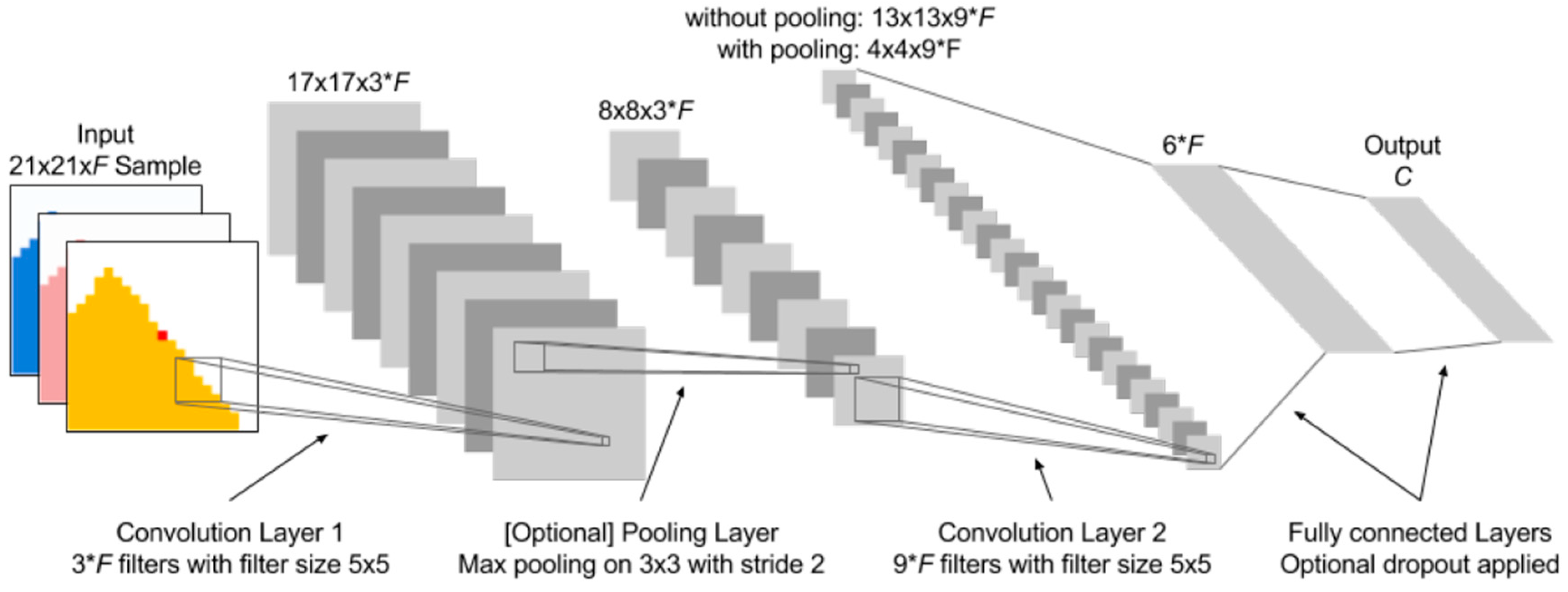
25] were able to produce good results on hyperspectral data with convolutional deep neural networks, we added this classification method to our experimental setup. Neural networks are inspired by the structure of the human brain to learn classification and regression tasks. A neural network consists of several layers of perceptron units that are interconnected. Via backpropagation, this network can learn from examples. A deep neural network has significantly more layers than a conventional network. Deep convolutional networks use filters that are shifted over the input image to generate new and more high-level features in each layer. It is not possible to test or even enumerate all possible network structures and parameter configurations. We therefore employed the network structure shown in
Figure 3, which is based on the one used in the original paper [
25]. The network starts with a convolutional layer containing
trainable filters (block size 5 × 5 pixels), where F denotes the number of features. The second convolutional layer then contains
trainable filters (block size 5 × 5). The output of this layer is then fed to a fully connected network with a hidden layer of size
. Additionally, we added the option to use a max-pooling layer in between the convolution layers and an option to apply a specified dropout rate to the fully connected network part. A pooling layer applies a filter mask for each pixel incorporating its surroundings. Common filters are mean or maximum filter. A dropout layer randomly omits a perceptron for the next training instance with a certain probability to avoid early convergence and to improve generalization. The deep learning library MatConvNet [
35] provided all functions needed to build our networks.
2.4. Fusion Algorithms
Equations (1) and (2) describe the applied framework for fusion of different base classifier results. Given a feature vector , its label is calculated as follows.
Using Equation (1), a score is calculated for each class label from the results of the N base classifiers. For each label in question, the score is a sum of weights for the corresponding base classifiers. The indicator function equals one, if its argument is true and zero, if not. Hence, only the weights of base classifiers with output label are included.
Equation (2) simply denotes the selection of the label with the highest score. Different voting strategies are implemented by variation of the weights .
Majority voting is defined by setting . If a majority of the base classifiers assigns the same label, the corresponding score is maximized. In our study, majority voting serves as a baseline for the performance of classifier fusion as it is a commonly used method.
Presidential voting is defined by setting and , where the index denotes a prior chosen classifier, e.g., the one with the best overall accuracy. Due to this constraint, the label assigned by the chosen classifier determines the ensemble result in most cases. Only if all other classifiers agree on the same divergent result, a different label is assigned.
Accuracy weighted voting uses a classification accuracy estimate to weight the different classifiers. According to the definitions in [
35], the average accuracy is calculated from the elements of the confusion matrix
of each classifier. A subset of the reference data is used to determine
and to estimate the weights
.
Hence, for the j-th classifier the weight
is defined with Equation (3) as the average accuracy [
36] which measures the average per-class effectiveness of a classifier.
The confusion matrix is transformed into confusion matrices to obtain the required true positive , true negative , false positive , and false negative values.
For precision weighted voting, a similar approach to calculate the weights is used. The precision measure is calculated with Equation (4) as follows
This fusion framework is a means to investigate how different popular approaches to weight a classifier influence the quality of the joint decision-making of an ensemble classifier.
3. Results
Table 4,
Table 5,
Table 6 and
Table 7 summarize the results of SVM, random forest, rotation forest, and CNN classifiers. Each table contains the mean accuracy values and standard deviations obtained with multiple runs of holdout testing. In the tables, for each feature space the best results per table row are emphasized as bold text. In addition, the feature space with the best overall classification accuracy is emphasized and the corresponding accuracy has been underlined. In each run, a complete reference site with a single dominant tree species was only used for testing the classifier, which was trained with data from the remaining reference sites. See
Table 1 for the total number of reference sites and areas. If only a single reference site is available it is divided into non-overlapping sites for training and validation of equal size. Each row corresponds to one of the selected feature spaces. We discriminate between the results of pixelwise and spatial classification, where statistical measures (mean, standard deviation, homogeneity) of the original features are used as features instead.
We report results for different ensemble sizes of random forest (
Table 5) and rotation forest (
Table 6) classifiers separately to assess the impact of this parameter and the trade-off for using a compact ensemble of 20 decision trees instead of a large ensemble of 100 decision trees.
Transformation of the reflectance data with MCLDA into a low dimensional representation yields the best results for all tested classifiers in separating between the 15 tree species. Moreover, inclusion of the spectral-spatial features significantly improves classification accuracy compared to pixelwise classification of spectral features in most cases. The best individual classifier was the CNN (see
Table 7) with an overall accuracy of 0.732 ± 0.086, followed by a rotation forest of 100 decision trees with an overall accuracy of 0.705 ± 0.044. The CNN intrinsically combines spectral and spatial information. Hence, the CNN operating on raw or preprocessed hyperspectral image data achieved a similar performance to fandom rorests and SVMs, which make use of handcrafted spectral and spatial-spectral features. However, even the CNN the initial transformation with MCLDA was crucial to achieve the gain in overall accuracy.
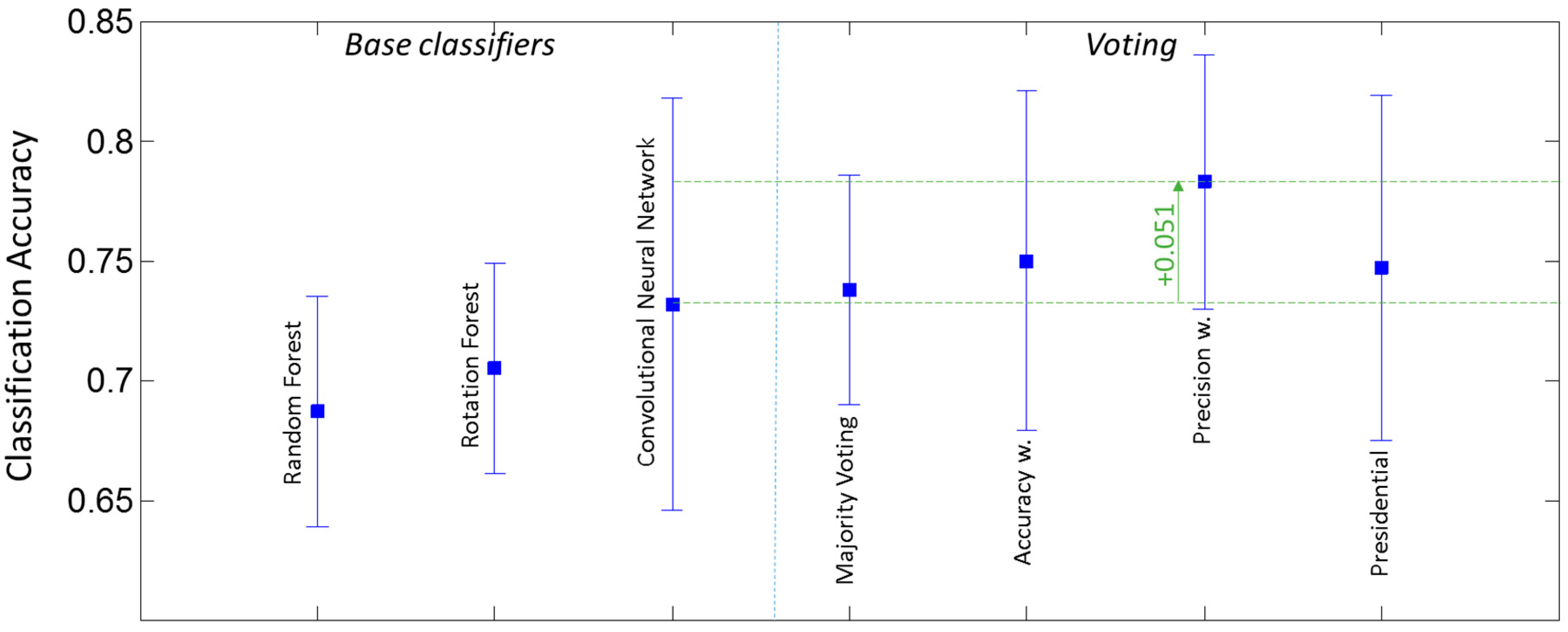
The results of combining a small number of base classifiers into a hybrid ensemble are summarized in
Figure 4. The diagram shows the accuracies and standard deviations of individual base classifiers together with results of different voting strategies. An accuracy gain of 5.1% was achieved by precision weighted voting compared to the best individual classifier. It significantly outperformed the three other tested voting methods.
To better understand these improvements,
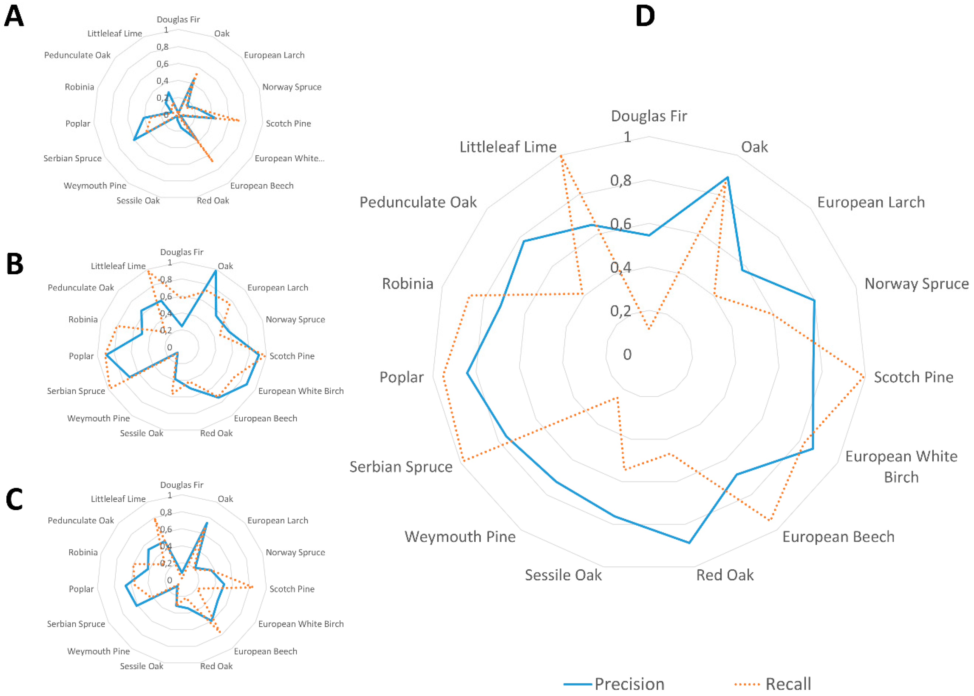
Figure 5 shows net diagrams of class-wise performance measures precision and recall. The subplots A–C show the performances of the included base classifiers, while subplot D represents the performance of the fusion framework with precision weighted voting using Equation (4) to calculate the weights.
The expected general improvement of class-wise precision values is shown by the more convex shape and the much larger area within the precision curve in subplot D. The recall value of the hybrid ensemble is still dominated by the best base classifier, the CNN (compare subplots B and D, dotted curves). However, a class0wise direct comparison reveals a few minor differences. For some tree species the recall values increase (e.g., poplar, robinia, oak), while for a few others (e.g., larch, Douglas dir) they decrease slightly.
4. Discussion
The need for a reliable tree species classification motivated our investigation of several state-of-the-art classifiers as well as their combination into an ensemble classifier. This demand has led to the development of a processing pipeline, where the positions of suitable training sites with one dominant tree species are obtained from existing databases of the forest authorities. Hence, it was possible to create a large training dataset covering 15 tree species without additional groundwork. The alternative, the assessment of tree species of individual trees in mixed forests by experts to create a reference database, either from ground or from aerial stereo imagery is expensive, time-consuming, and error-prone.
Although, we developed a promising framework for classifier fusion and did careful validation, the method was not validated against ground truth data from real mixed forests. This is due to the fact that a large-scale validation would require the same efforts to obtain the reference data as mentioned above for the classifier training. However, the method was successfully applied to classify the complete forest in our hyperspectral dataset. This tree species map can then be used to select a number of individual trees and to validate the assigned class label in the field.
The performance of classification models based on this kind of training data was extensively tested with a combination of cross-validation and hold-out-testing. Compared to standard cross-validation not only a subset of randomly chosen pixels or patches were excluded from training for testing, but complete areas. This allowed us to study the performances on independent data. However, the spectral data belongs to a single measurement flight and has undergone the same preprocessing (e.g., radiometric and atmospheric corrections). Hence, the trained classifiers are adapted to the development stages of the trees and the conditions on the day of flight. To our best knowledge, the proposed method to acquire training data directly from the hyperspectral images at predefined locations with dominant tree species is the best way to learn classification models for future flights. Otherwise, many test flights and expenses are required to acquire training data that cover all possible appearances of leaves and needles beforehand. Locations with a single dominant tree species can be determined by an expert using existing databases and aerial images. For any region, this could be done once stored in a database and then be used for future measurement flights.
The per-class assessment of the classification performance of the fusion approach shows differences depending on the tree species. The net diagram in
Figure 5 reveals that the precision of the class assignment was improved to large extends, but for some tree species the fraction of successfully detected trees remains low. However, compared to the state-of-the-art CNN a significant loss is only observed for Douglas firs. On the other hand, the rate of true Douglas firs among the reported ones increased significantly. There are different reasons, which possibly explain this behavior. First, the dataset contains a number of tree species with only subtle differences like oaks, sessile oaks, red oaks, and pedunculate oaks. While this information is of interest for the forest authorities and motivates the use of hyperspectral imaging to detect subtle differences, it might be better to take a hierarchical approach, which first detects all oaks and then tries to discriminate between oak species. Second, some of the tree species are more common than others. We account for this by balancing the dataset to have an equal number of samples for all tree species. However, the number of reference sites for rare species is also low and the natural variation between trees is better covered for frequent tree species. Here, our strict validation with holding back complete reference sites for testing may penalize the rare species.
With Scotch pines, Norway spruces, oaks, and beeches being the most frequent tree species in Saxony-Anhalt as well as Thuringia the results show, that our approach for analysis of airborne hyperspectral images already provides a useful tool to support forest inventory and to detect oak trees for subsequent analysis of vitality parameters. Moreover, the proposed fusion framework allows to easily add any other classifier.

 ,
, 


