Midterm Fire Danger Prediction Using Satellite Imagery and Auxiliary Thematic Layers

Abstract

Wildfires constitute a significant environmental pressure in Europe, particularly in the Mediterranean countries. The prediction of fire danger is essential for sustainable forest fire management since it provides critical information for designing effective prevention measures and for facilitating response planning to potential fire events. This study presents a new midterm fire danger index (MFDI) using satellite and auxiliary geographic data. The proposed methodology is based on estimations of a dry fuel connectivity measure calculated from the Moderate Imaging Spectrometer (MODIS) time-series data, which are combined with biophysical and topological variables to obtain accurate fire ignition danger predictions for the following eight days. The index’s accuracy was assessed using historical fire data from four large wildfires in Greece. The results showcase that the index predicted high fire danger (≥3 on a scale within $[1,4]$) within the identified fire ignition areas, proving its strong potential for deriving reliable estimations of fire danger, despite the fact that no meteorological measurements or forecasts are used for its calculation.

1. Introduction

Forest fires are considered a rather complex natural process and one of the most crucial environmental issues in Europe [1], resulting in severe ecological, economic, and social consequences [2]. Most of the total European fire-affected areas are located in the Mediterranean countries during the summer season [2,3,4]. For example, Portugal, Spain, France, Italy, and Greece accounted for 78% of the total burnt area and 84% of the total number of fires registered in Europe in the 2000–2013 period, according to Burned Areas Perimeters dataset of the European Forest Fire Information System (EFFIS) [4]. For the five larger southern European countries most affected by wildfires (Portugal, Spain, France, Italy, and Greece), the number of fires has increased from 1980 to 2000 (partly due to improvements in monitoring systems) and has decreased afterwards (which is partly attributed to the improvement of the fire suppression mechanism), albeit with considerable variability in both number of fires and total area burned each year [5,6]. Nevertheless, climate change is expected to result in increased temperatures and prolonged droughts that may, in turn, lead to a major increase in the frequency and severity of fires [5,7], not only in the Mediterranean countries but also in northerner European countries as well.

Reliable fire danger forecast constitutes one of the most significant components of integrated forest fire management [8] and it is highly dependent on a variety of factors affecting fire ignition and spread. These factors comprise meteorological variables, vegetation condition, topography, and human activities, which are utilized as inputs in existing fire behavior prediction systems (e.g., Fire Area Simulator—FARSITE, FlamMap, FS Pro) [8,9]. Weather is considered the most dynamic factor affecting fire danger as it influences fuel moisture content—mostly that of the dead fuels—and partly determines wind direction [10,11]. Therefore, most of the eminent operationally applied fire danger forecasting systems are primarily based on meteorological data measurements and/or predictions [8]. The Canadian Forest Fire Danger Rating System (CFFDRS) [12], the National Fire Danger Rating System (NFDRS) adopted in the USA [13], and the Australian McArthur rating systems [14] are some of the most widely used operational systems providing forecasts of potential fire ignition, behavior, and rate of spread [15,16].

When the aforementioned fire danger forecasting systems are to be applied in a new ecosystem, they should be evaluated and—if required—calibrated to the meteorological conditions and vegetation cover of the new area [8,17,18]. A number of recent studies have investigated the suitability of existing operational fire danger indices in different countries. Horel et al. [19] evaluated the CFFDRS indices that were calculated in the framework of the Great Lakes Fire and Fuel Information System (GLFF) in the United States. The researchers concluded that most of the calculated CFFDRS values are comparable to those derived from observations whereas precipitation-related indices are more prone to errors. De Long et al. [20] introduced a percentile-based calibration approach for the Canadian Forest Fire Weather Index (FWI) System in the United Kingdom. The results showcased that the Fine Fuel Moisture Code (FFMC), Initial Spread Index (ISI) and FWI components of the FWI System performed better compared to the rest of the system’s components, namely the Duff Moisture Code (DMC), the Drought Code (DC) and the Buildup Index (BUI). Beccari et al. [21] examined the potential of the FWI in the Alpine region for its integration within a new fire risk occurrence model. Different fire danger indices (e.g., Nesterov, Telicyn, and FWI) were also evaluated in Brazil [11], with varying results across the different states of the country.

Apart from performance evaluation and calibration of existing fire danger indices, researchers have focused on the development of new ones based on meteorological variables for the reliable forecast of fire danger conditions in a variety of ecosystems. Sharples et al. [22] introduced a new index for fire danger rating in Australia, which was compared to a number of other indices operationally applied in Australia and the United States (e.g., McArthur Mark 4 and Mark 5 Grassland Fire Danger Meters and the Fosberg FWI) and exhibited satisfactory accuracy. Bellis et al. [23] ) designed a platform for fire risk prediction based on the Australian McArthur index with—as stated by the authors–acceptable performance. Furthermore, multivariate linear regression modeling was applied for the development of a reliable method for forest fire forecast, based on measurements from wireless sensor networks [24].

Whereas weather-based fire danger systems constitute an appropriate tool for civil protection agencies and other relevant authorities, information related only to the meteorological conditions of an area is not enough for accurate fire danger prediction and rapid response in case of a potential fire event [25]. The use of additional fire-affecting factors such as the fuel types, their condition, and the topography of the area is essential [25,26]. Moreover, the volume of meteorological data required by the aforementioned operational forecasting systems is large and their calibration requires extensive ground data collections [27]. The meteorological variables used by most of these systems are obtained from weather stations that provide information solely for point locations [8,28]. Hence, surface maps for the variable of interest are produced through the application of GIS-based interpolation techniques, but such an approach results in different outputs being produced using the same input variables [8,29]. Especially in cases where the distance between two weather stations is more than 20 km, interpolation methods may not produce reliable results for the areas between the stations [30]. Another limitation of using only point-based meteorological data is that weather stations are often sparsely located, which means that continuous spatial coverage cannot be achieved, especially in the case of remote forested areas [31].

The aforementioned limitations and uncertainties about the results’ accuracy can be alleviated with the use of satellite remote sensing. Satellite remote sensing technologies have the advantage of capturing the spatial–spectral variability on a regular basis and over extended and/or remote areas [32,33,34]. In the last decade, satellite remote sensing has been investigated for its applicability in reliable forecasting of fire danger conditions, either by employing the remotely-sensed data alone or combining them with meteorological variables [33,35,36].

With respect to fire danger estimation methodologies that incorporate meteorological variables, Yu et al. [37] employed both remote sensing and meteorological variables for fire risk forecast in Cambodia. They combined MODIS-derived products with Shuttle Radar Topography Mission (SRTM)-derived DEM and Tropical Rainfall Measuring Mission (TRMM)-derived precipitation data reporting good agreement between the predicted risk and MODIS-derived fire spots. Moreover, Landsat satellite imagery was employed by Mitri et al. [38] for the generation of a land use/cover map, which was combined with other biophysical and WorldClim data (e.g., average monthly climate data for minimum, mean, and maximum temperature, and precipitation) [39] in order to reliably predict wildfire risk in the Lebanon region. The methodology was later enhanced by combining the initial fire risk data with drought spatial characteristics extracted from the WorldClim database, topographic, socio-economic, and fire data, leading to the development of a new daily fire danger index for the Lebanon region [26]. In another study [40], weather variables provided by 45 meteorological stations, vegetation data derived from Landsat and IKONOS satellite images, as well as other anthropogenic, topographic, and fire data were fed as inputs into a multi-layer perceptron, in order to accurately map regional forest fire probability in a Mediterranean ecosystem. DaCamara et al. [41] introduced a methodology for operational generation of fire danger maps over the Mediterranean Europe using vegetation cover maps obtained from Global Land Cover 2000 (GLC2000) dataset, meteorological data provided by the European Centre for Medium-Range Weather Forecasts (ECMWF) operational model, and fire activity based on the Fire Detection and Monitoring (FD&M) product from the Satellite Application Facility on Land Surface Analysis (LSA SAF) [42]. Chowdhury and Hassan [34] used MODIS-derived environmental variables, such as daily perceptible water (PW), Ts, and Normalized Difference Vegetation Index (NDVI) for the development of a daily fire danger forecasting system.

Focusing on methodologies not relying on meteorological variables directly, Abdollahi et al. [43] employed MODIS-derived products and historical fire ignition data for the performance enhancement of an existing fire danger forecasting system (FFDFS) that is solely based on remote sensing data. MODIS vegetation and canopy water content-related indices were analyzed by Arganaraz et al. [44] for live fuel moisture estimation and the subsequent prediction of fire danger conditions in Argentina. Matin et al. [45] integrated several factors related to land cover, surface temperature, topography, and spatial proximity to human activities using MODIS satellite imagery and Geographic Information System (GIS) to generate a fire risk map covering the area of Nepal. MODIS data were also employed for land cover mapping of the Uttarakhand state of India [46]. The produced vegetation map was used to produce a fuel type danger index, which was subsequently combined with various topographic variables (i.e., elevation, slope, aspect, and terrain ruggedness) for the generation of the final so-called Static Fire Danger Index, the accuracy of which approached $95\%$. Babu et al. [47] developed a fire danger index mainly based on MODIS-derived parameters (e.g., Land Surface Temperature, Normalized Multiband Drought Index, Modified Normalized Difference Fire Index), which is currently operationally employed in Kazakhstan. Liu et al. [48] used MODIS surface temperature (Ts) and reflectance data in combination with Advanced Spaceborne Thermal Emission and Reflection Radiometer (ASTER)-derived DEM and historical lightning-caused fire data for fire risk forecast over a mountainous area in China. MODIS 16-day enhanced vegetation index (EVI) and daily Ts were integrated by Bisquert et al. [49] to predict fire danger conditions over the Galicia region in Spain for the period 2001-2006. Akther and Hassan [50] evaluated different satellite-based variables/indices to predict fire danger over boreal forests of Alberta for the period 2006–2008, proving that the combined use of Ts, normalized multiband drought index (NMDI) and temperature vegetation wetness index (TVWI) results in accurate ($91.63\%$) fire danger predictions. Ahmed et al. [51] introduced a new model for forest fire danger prediction in northern Alberta on a four-day basis using three different Terra MODIS products (i.e., surface reflectance, land surface temperature, land cover map). The results showcased high agreement with the historical fire data revealing its’ strong potential for operational use.

Most of the aforementioned fire danger forecasting systems provide daily fire danger estimations, i.e., they forecast the next day’s fire danger conditions. Fire danger assessment on a midterm basis is also of high importance and could be synergistically employed with the daily estimations, aiding stakeholders to apply the appropriate prevention management practices. Here, we consider as midterm the fire danger forecasts that cover a period of at least one week ahead from the day they are issued. The number of such midterm indices that do not rely on meteorological measurements or predictions is still limited in the literature [34].

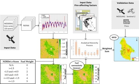
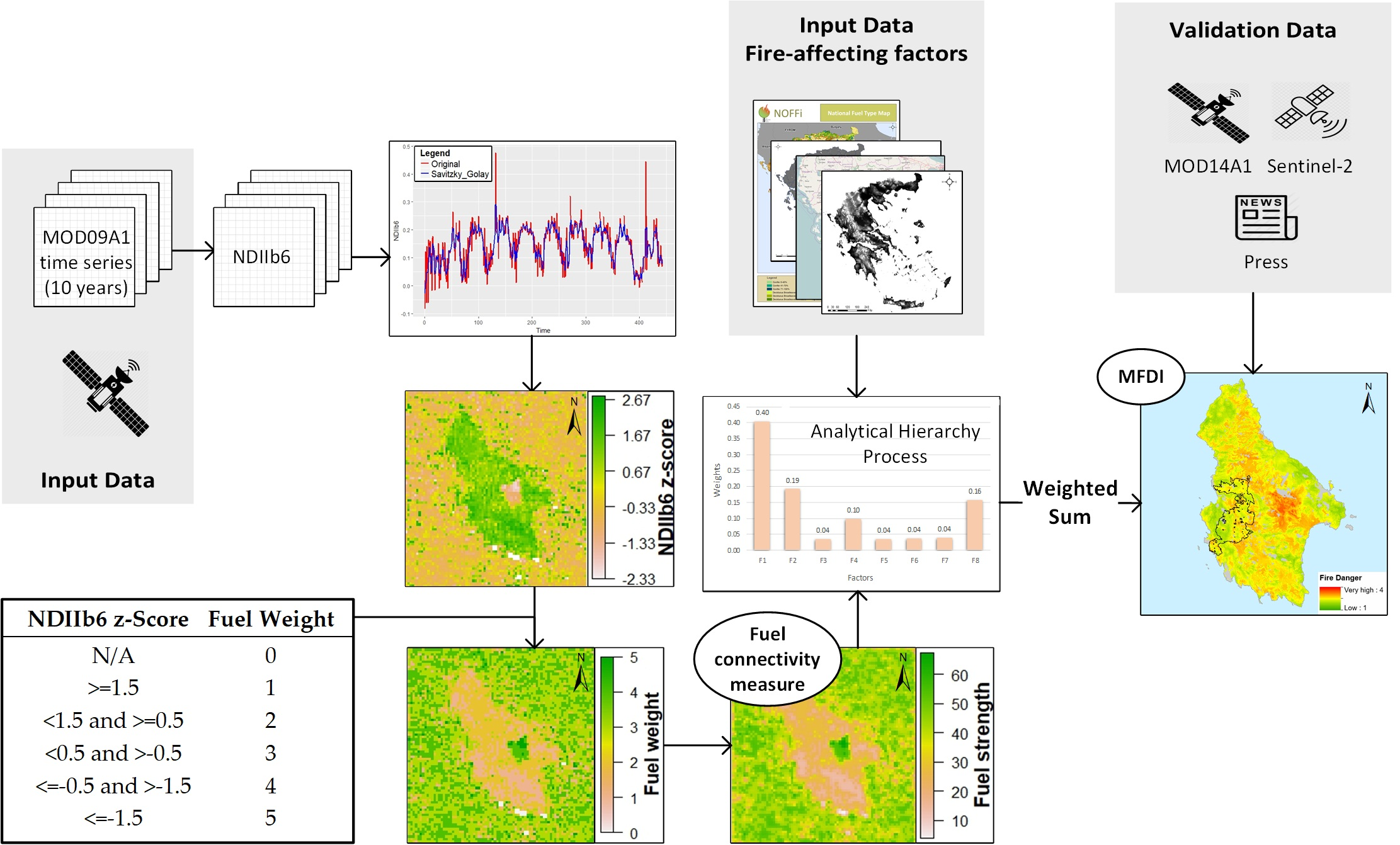
This study presents a new midterm fire danger index (MFDI) for a Euro-Mediterranean region (Greece), which is based on Earth Observation and ancillary geographic data and provides reliable estimations of fire ignition danger for a period of eight days ahead without using any meteorological data. Our methodology builds upon a previously proposed automated method for monitoring the spatial dry fuel connectivity [52] and combines it with additional biophysical and topographic variables for fire danger forecast on a midterm basis. Considering the spatial heterogeneity of vegetation patterns, the diversity of tree species, and the topographical variability characterizing the Mediterranean ecosystems [53], the spatial resolution of the fire danger maps is crucial for the accurate representation of fire danger conditions. The dry fuel connectivity estimates are considered as the main component of MFDI and provide information of 500 m spatial resolution, whereas all the other integrated variables have a spatial resolution of 30 m.

2. Materials and Methods

Figure 1 provides an overview of the proposed methodology. Time-series of MODIS satellite data—spanning the 10 previous years—are used to identify extrema in vegetation moisture content. This is achieved by first calculating a moisture-sensitive spectral index from the original MODIS bands and then deriving a so-called fuel connectivity measure, taking into consideration the index’s deviation relative to the 10 years history as well as the respective values from its spatial neighbors. The fuel connectivity measure is combined with other static variables (fuel type, topographic features, and distance from specific land cover/use classes) by means of the analytic hierarchy process [54] multi-criteria analysis, thus deriving the proposed fire danger index. The accuracy of the latter is finally assessed considering a number of test cases in Greece and various sources of information. The rest of this section describes in detail each individual step.

2.1. Datasets

The EO datasets required for MFDI are eight-day composite surface reflectance products from the MODIS sensor (MOD09A1). MOD09A1 provides an estimate of surface spectral reflectance values of Terra MODIS bands 1–7 (at a spatial resolution of 500 m), corrected for atmospheric conditions, along with a quality flag layer and four observation bands [35]. The products were downloaded from the MODIS Global Subsets Tool of the Oak Ridge National Laboratory Distributed Active Archive Center (ORNL DAAC) (https://modis.ornl.gov/cgi-bin/MODIS/global/subset.pl) for a ten-year period for each case study. Official perimeters of the burned areas within the study area are also necessary for the application of the proposed method. These data were provided by the Greek Ministry of Environment and Energy and the Laboratory of Forest Management and Remote Sensing (FMRS) of the Aristotle University of Thessaloniki in Greece.

The midterm prediction of fire danger also necessitates spatial information regarding the type and distribution of fuels, which constitutes one of the most important parameters that directly affect fire ignition and propagation danger. A national fuel type map (with 30 m spatial resolution) was developed in the framework of the NOFFi project (http://epadap.web.auth.gr/?lang=en), using the Landsat 8 OLI satellite imagery and ancillary spatial layers, such as the official national vegetation layer provided by the Hellenic Ministry of Environment and Energy [36]. The mapping process was performed through the development of an object-based Image Analysis (OBIA ) model [55] based on fuzzy logic rules, which was applied in all regional units to derive a country-wide map. The validity of the map was assessed using control points from the land use and land cover area frame survey (LUCAS) provided by Eurostat and the overall accuracy reached $92.59\%$ [36].

The boundaries of urban and agricultural areas extracted from the Land Parcel Identification System (LPIS) geodatabase are also required and have been provided by the Hellenic Agricultural Payments Organization (OPEKEPE) in accordance to the European Union’s (EU) Common Agricultural Policy (CAP). In addition, the Advanced Spaceborne Thermal Emission and Reflection Radiometer (ASTER) Global Digital Elevation Model (GDEM) (https://asterweb.jpl.nasa.gov/gdem.asp) (30 m spatial resolution) and the OpenStreetMap (OSM) road network are also considered as fire-influencing parameters for the MFDI computation.

Finally, the validation procedure required the use of additional satellite data, namely the MODIS thermal anomalies and fire products and Sentinel-2 satellite images. The MODIS active fire product (MOD14A1) is a composite of fire pixels at 1 km spatial resolution detected in each cell of a predefined grid with a daily period [56]. MOD14A1 is produced every eight days but includes daily information, i.e., complete per-pixel information for each of the corresponding eight days [56]. The pixels are classified in ten categories according to

Table 1. MOD14 fire mask pixel classes [56].

Class	Description
0	Not processed (missing input data)
1	Not processed (obsolete; not used since Collection 1)
2	Not processed (other reason)
3	Non-fire water pixel
4	Cloud (land or water)
5	Non-fire land pixel
6	Unknown (land or water)
7	Fire (low confidence, land or water)
8	Fire (nominal confidence, land or water)
9	Fire (high confidence, land or water)

[56]. Sentinel-2 is a European satellite mission within the Copernicus EO program, providing high-resolution multi-spectral imagery from two identical sensors with a revisit frequency of five days. The Sentinel-2 product consists of 13 spectral bands, four of which are at 10 m spatial resolution, six at 20 m and three at 60 m [57]. Sentinel-2 images were used in two test cases, at which the imager captured the fire ignition areas.

Table 2. Satellite data used in this study.

Name	Product ID	Spatial Resolution	Temporal Resolution
Surface Reflectance	MOD09A1	500 m	8 days
Active Fire	MOD14A1	1 km	daily
Surface Reflectance	Sentinel-2	10 m	5 days
Digital Elevation Model	ASTER GDEM	30 m	−

and

Table 3. Vector data used in this study.

Name	Extracted Information
National fuel type map	Spatial distribution of forest fuels
Burned areas	Historical fire perimeters
Land Parcel Identification System (LPIS)	Agricultural and urban areas
OpenStreetMap (OSM)	Road network

provide a brief description of all datasets used in the present study.

2.2. Methods

The proposed method includes two main parts (Figure 1), namely the estimation of the dry fuel spatial connectivity and the combination of these estimates with ancillary data for the calculation of the MFDI fire danger rating. Both parts of the method have been implemented in the free and open-source software R, compiled into an automated workflow.

2.2.1. Dry Fuel Spatial Connectivity Estimation

The dry fuel connectivity constitutes a precipitation-driven variable and its estimation follows the automated procedure introduced in [52]. The measure is based on the Normalized Difference Infrared Index—band 6 (NDIIb6), which is calculated using the first short-wave infrared (SWIR) band (Band 6) of the MOD09A1 product:

$$\mathrm{NDIIb}6=\frac{\mathrm{Band}2-\mathrm{Band}6}{\mathrm{Band}2+\mathrm{Band}6},$$

(1)

where Band2 and Band6 are the MODIS near-infrared (841–876 nm) and SWIR (1628–1652 nm) reflectance values, respectively. NDIIb6 is highly correlated with canopy water content, which is one the most important fire-affecting vegetation characteristics, since moisture constrains flammability and fire spread [52,58,59,60]. It is a normalized index and the values theoretically range between $-1$ and 1, with the lower values (especially below zero) indicating canopy water stress [60].

The NDIIb6 is calculated for the whole MODIS time-series (ten-year period). Data anomalies (e.g., clouds) are masked out using the quality assurance (QA) metadata (state QA flag) [35]. Any residual noise and atmospheric disturbances affecting the time-series is eliminated by means of the adaptive Savitzky-Golay smoothing filter [61].

The smoothed time-series is subsequently used for calculating the z-score of the NDIIb6 values, expressed as the deviation from the mean value over the examined ten-year period (NDIIb6 anomaly data). If y is the current year, $m_{kx}$ is the average NDIIb6 value over the previous ten years for image pixel k and for the specific eight-day composite x ($x\in [1,46]$, covering a whole year), i.e., $m_{kx}=0.1·{\sum }_{i=y-10}^{y-1}{\mathrm{NDIIb}6}_{kxi}$, and ${\sigma }_{kx}$ is the corresponding standard deviation, the z-score is defined as:

$$z_{kxy}={\displaystyle \frac{{\mathrm{NDIIb}6}_{kxy}-m_{kx}}{{\sigma }_{kx}}}.$$

(2)

The rationale for using the z-scores instead of the absolute NDIIb6 values is that fire danger conditions are linked to these NDIIb6 anomaly data (i.e., relative deviations), rather than the absolute index values [28,52,62,63], since the former represent the drought-induced anomalies, at least as quantified by the pixel’s spectral response [28]. In other words, the higher the drought anomalies (low NDIIb6 z-score values), the higher the fuel flammability potential is and, consequently, the greater the danger for a fire to occur is. The normalization of these deviations (division with the standard deviation) allows the subsequent categorization of the z-score values into six dryness classes, with an integer fuel weight being assigned to each one of them (high fuel weights representing drier fuels), as reported in

Table 4. Dryness classes and fuel weights based on NDIIb6 z-score ranges [52].

Dryness Class	NDIIb6 z-Score	Description	Fuel Weight
1	N/A	Time since last fire <5	0
2	$\ge 1.5$	Severely wet	1
3	<1.5 and $\ge 0.5$	Wet	2
4	<0.5 and >−0.5	Normal	3
5	≤−0.5 and > −1.5	Dry	4
6	≤−1.5	Severely dry	5

.

Fire danger is not only affected by the drought status of a small area such as that of a pixel, but also from the state of neighboring pixels. Imagine, for example, that a pixel has a very low z-score value (i.e., abnormally dry), but all neighboring pixels have medium or high z-score values. In this case, the probability of a fire to start and spread from the central pixel is lower than that implied by its very low z-score value. Following this reasoning, the aforementioned fuel weight image is processed in order to estimate the dry fuel connectivity map, considering a $3\times 3$ pixel neighborhood around each pixel. The weight of each connection between the central pixel and one of its neighbors is computed by summing their fuel weight values. For the four diagonal connections, this sum is further divided by $\sqrt{2}$, accounting for the longer distance [52,64]. Finally, the fuel strength (connectivity measure) of each pixel is calculated by summing the weights of all connections with its eight neighboring pixels. In other words, areas with high fuel strength represent more strongly connected dry fuels, which leads to higher fire danger.

Mathematically, the calculation of the dry fuel connectivity is performed as follows:

$$W_{i,j}={\mathbf{1}}^{\mathrm{T}}\times ({\mathbf{P}}_{i,j}\circ {\mathbf{F}}_{i,j}\times \mathbf{1}),$$

(3)

where ${\mathbf{W}}_{i,j}$ is the dry fuel connectivity for the pixel located at row i and column j of the fuel weight image, $\mathbf{1}$ is a column vector of ones, ${\mathbf{1}}^{\mathrm{T}}$ is its transpose, ∘ denotes the Hadamard product (also known as Schur or entry-wise product), ${\mathbf{P}}_{i,j}$ is the matrix of pixel values in the neighborhood of the pixel located at row i and column j of the fuel weight image:

$${\mathbf{P}}_{i,j}=\left[\begin{array}{ccc}{p}_{i-1,j-1}& p_{i-1,j}& p_{i-1,j+1}\\ p_{i,j-1}& p_{i,j}& p_{i,j+1}\\ p_{i+1,j-1}& p_{i+1,j}& p_{i+1,j+1}\end{array}\right]$$

(4)

and ${\mathbf{F}}_{i,j}$ is the following weighting matrix:

$${\mathbf{F}}_{i,j}=\left[\begin{array}{ccc}1/\sqrt{2}& 1& 1/\sqrt{2}\\ 1& 4+4/\sqrt{2}& 1\\ 1/\sqrt{2}& 1& 1/\sqrt{2}\end{array}\right]$$

(5)

The dry fuel connectivity estimates ($W_{i,j}$) are used as the component related to vegetation dryness in the proposed MFDI. This is subsequently combined with the other input parameters through multi-criteria analysis detailed in the following section.

2.2.2. Multi-Criteria Analysis

The second part of the methodology comprises the application of the Analytical Hierarchy Process (AHP) for estimating the final fire danger rating. AHP is a multi-criteria decision-making method that employs pairwise criteria comparisons in order to determine a scale of preferences among different sets of alternatives [54]. Numerical values representing the relative importance of one factor against all others are assigned to each factor, according to a judgment scale (for example, linear), so that they can be compared to each other in a pairwise comparison matrix [54,65].

Saaty’s pairwise comparison scale (

Table 5. Saaty’s pairwise comparison scale [54].

Intensity of Importance	Definition
1	Equal importance
3	Weak importance of one over another
5	Essential or strong importance
7	Demonstrated importance
9	Absolute importance
2, 4, 6, 8	Intermediate values between the two adjacent judgements
Reciprocals of above zero	If activity i has one of the above nonzero numbers assigned to it when compared with activity j, then j has the reciprocal value when compared with i

) [54,66] was used for the development of the pairwise comparison matrix. It is a nine-valued scale that quantifies the relative importance between any two criteria in a multi-criteria decision system, based on the linguistic description of an expert. If the importance of a criterion over another has been graded with some value by the expert, the reciprocal value is used by definition when comparing the criteria in the reverse order. The criteria compared to each other include the fuel connectivity estimates, fuel types, distance from agricultural areas, urban areas and road network, elevation, slope, and aspect. The relative importance values have been determined through expert knowledge and the results are reported in

Table 6. Pairwise comparison matrix developed using the Saaty’s pairwise comparison scale (C1 = fuel connectivity, C2 = fuel type, C3 = elevation, C4 = slope, C5 = aspect, C6 = proximity to roads, C7 = proximity to urban areas, C8 = proximity to agricultural areas).

Criteria	C1	C2	C3	C4	C5	C6	C7	C8
C1	1.00	5.00	7.00	7.00	7.00	9.00	9.00	7.00
C2	0.20	1.00	5.00	5.00	9.00	9.00	7.00	0.33
C3	0.14	0.20	1.00	0.20	0.33	3.00	0.33	0.20
C4	0.14	0.20	5.00	1.00	5.00	3.00	5.00	0.33
C5	0.14	0.11	3.00	0.20	1.00	0.50	0.50	0.20
C6	0.11	0.11	0.33	0.33	2.00	1.00	2.00	0.33
C7	0.11	0.14	3.00	0.20	2.00	0.50	1.00	0.20
C8	0.14	3.00	5.00	3.00	5.00	3.00	5.00	1.00
Total	1.99	9.77	29.33	16.93	31.33	29.00	29.83	9.60

. The validity of the latter has been confirmed by calculating the so-called consistency ratio (CR), the most well-known measure employed to quantify the consistency of the comparison matrix in AHP [66,67]. In our case, the CR was calculated as 0.17, which is considered acceptable [68,69,70,71]. Therefore, no further reevaluation of the expert’s judgments was performed, and the comparison matrix was considered as acceptable.

The relative factor priorities (weights) are derived by first normalizing the comparison matrix’s columns (by dividing each column with its sum) and then calculating averages for each row [66]. The resulting weights in our case are reported in

Table 7. Fire danger weight for each parameter as calculated through the analytical hierarchy process (AHP).

Parameters	Fire Danger Weight
Fuel connectivity	0.40
Fuel type	0.19
Elevation	0.03
Slope	0.10
Aspect	0.04
Road network	0.04
Urban areas	0.04
Agricultural areas	0.16

. Obviously, the fuel connectivity factor received the highest relative weight, since it was rated as the most important among all factors by the expect (values greater than one in the first row of Table 6). Fuel type received the second-highest weight, closely followed by proximity to agricultural areas, since a substantial number of wildfires in the Mediterranean area start from human activities in agricultural areas [72,73].

In order to derive the final MFDI estimations, all spatial datasets used to calculate the factors of Table 7 (see Section 2.1) must be co-registered into a common spatial grid and converted into a common metric scale. For the latter, we chose to employ a four-valued ordinal scale from 1 to 4 (i.e., 1 = low, 2 = moderate, 3 = high, 4 = very high), frequently used in fire danger forecasting systems [46,50,74].

The slope and aspect rasters are generated by the DEM raster (which provides the elevation information). The linear vector features of the road network and the polygons of the agricultural and urban areas are used for the derivation of the raster datasets (with a spatial resolution of 30 m, co-registered with the DEM raster) representing the Euclidean distance to the closest source, i.e., proximity to roads, agricultural, and urban areas. Finally, the dry fuel connectivity raster (500 m spatial resolution) is resampled to 30 m (following the nearest neighbor resampling approach) and co-registered with the DEM raster as well.in order to match the spatial resolution of all other raster datasets. All input variables are subsequently classified to the aforementioned four-valued ordinal scale, following the reclassification procedure reported in

Table 8. Discretization of each parameter (dry fuel connectivity, fuel type, elevation, slope, aspect, proximity to agricultural areas, urban areas and road network) according to a common risk scale (1 = low, 2 = moderate, 3 = high, 4 = very high).

Parameter	Class/Range/Process	Common Risk Scale Value
Dry fuel connectivity	Linear transformation	1–4
Fuel type	Water and not vegetated areas	—
	Agricultural areas	4
	Low vegetation	3
	Shrubs	3
	Conifer 10–40% Sparse	2
	Conifer 41–70% Dense	2
	Conifer 71–100% Very dense	2
	Evergreen broadleaf 10–40% Sparse	3
	Evergreen broadleaf 41–70% Dense	2
	Evergreen broadleaf 71–100% Very dense	2
	Deciduous broadleaf 10–40% Sparse	2
	Deciduous broadleaf 41–70% Dense	1
	Deciduous broadleaf 71–100% Very dense	1
Elevation (m)	0–100	4
	101–500	3
	501–1000	2
	>1000	1
Slope (%)	0–20	4
	21–50	2
	>50	1
Aspect	North (315–360°and 0–45°)	1
	East (45–135°)	2
	South (135–225°)	4
	West (225–315°)	2
Proximity to roads and urban areas (m)	≤500	4
	>500	1
Proximity to agricultural areas (m)	<100	4
	100–300	3
	>300	1

. Following the example of other relevant studies (e.g., [38,43,75,76,77]), the thresholds used to categorize continuous variables into fire ignition danger classes or the reclassification of nominal variables are based on expert fire knowledge and experience taking into account the index objective—which is to classify fire ignition danger—as well as the ecosystem type for which the index is developed (i.e., Mediterranean). More specifically, the reasoning followed for each parameter is summarized in the following points:

• The fuel connectivity measure is confined in the range $[0,68.28]$, which can be obtain if Equations (3)–(5) are employed with all elements of matrix ${\mathbf{F}}_{i,j}$ having the minimum (0) or maximum (5) z-score fuel weight value (see Table 4). This range is simply linearly mapped to the (continuous) range $[1,4]$.
• Regarding fuel types, agricultural areas were assigned the highest risk value, since a substantial number of wildfires in the Mediterranean area start from human activities in agricultural areas [72,73]. Low vegetation, shrubs, and sparse evergreen broadleaved vegetation were assigned a high-risk value, because they dry easier than other vegetation types during the summer months, increasing their flammability. Conversely, dense or very dense deciduous broadleaved forests received the minimum risk value, since they are characterized by increased moisture content throughout the whole fire season. All other fuel type categories received a moderate risk value. This classification of fuel types with respect to fire ignition risk is consistent with the results of various studies in Mediterranean ecosystems (e.g., [73,78,79,80]). We should note that water and non-vegetated areas are not assigned any risk level, so they proposed MFDI is not calculated for those areas (since they are not burnable).
• Regarding topography, lower altitudes are significantly more prone to fires, with the risk becoming negligible above 1000 m [81]. Although the fire spread risk increases at steeper slopes, we chose to assign decreasing wildfire ignition risk values as the terrain’s slope increases, because human activities are concentrated mainly in flat terrains (urban interfaces, road network, agricultural activities, etc.) [82,83]. As for terrain aspect, south-facing slopes exhibit the highest ignition risk—since they receive higher direct solar energy during the day [84]—and conversely, northern aspects the lowest risk, whereas eastern and western aspect have an intermediate (to low) risk [79,85,86].
• A buffer of 500 m around the road network is frequently considered as a high-risk zone for wildfires ignitions [43,73,81,87] and the same threshold was also applied for proximity to urban areas. With respect to agricultural land, the higher the proximity to these areas the greater the danger of fire ignition [88]. Following this general rule and considering the fire ignition drivers in Greece, empirical thresholds based on expert knowledge and experience were considered for defining the three distance zones, see Table 8.
• In assigning the discrete values, each parameter is considered independently from the others and the minimum (1) and maximum (4) values are always assigned to the extreme categories. When a parameter has been split into three categories (e.g., proximity to agricultural areas), the intermediate category receives the value closer to the more appropriate extreme, as decided by the expert.

Having transformed all parameters into a common scale, the final MDFI value is derived via a weighted sum of all variables, using the weights obtained by the AHP (Table 7).

2.2.3. Accuracy Assessment

The validation of MFDI was based on historical fire events of four large wildfires in Greece, namely, in the Attica region (fire of June 2007), in two areas at Euboea Island (Karistos and Farakla for the fires of July 2016), and one at Kythira Island (fire of August 2017). The ten-year analysis period varies in each case study according to the year of fire occurrence, ranging from the MODIS eight-day composite ten years prior to the fire event until the one before the eight days period for which fire danger is being estimated. Thus, MODIS time-series data for the period 2007–2016 were employed for Karistos and Farakla areas at the Euboea island and 2008–2017 for the Kythira island. As for the Attica region, the lack of availability of a full MODIS time-series before 2001 led to the analysis of the period 2001–2010. The decision of using the specific time range was based on the assumption that the trend of drought under current climate conditions remains unchanged between the two time periods (1998–2007 and 2001–2010).

Ideally, MFDI’s validation would have to be performed considering a large number of fire ignition points from historical wildfires. However, these data could not be provided to us by the Greek Fire Service that maintains this database, due to legal restrictions. As such, we used the aforementioned four historical fire events instead, for which we were able to identify the ignition points by other means. In the case of Karistos (Euboea region), we employed the MODIS active fire product (MOD14A1), comparing the average MFDI value within all MOD14A1 pixels flagged as fire (high confidence) with the average MFDI value over the rest of the burned area. Although the use of the MOD14A1 may seem as a systematic approach in validating MFDI, in practice it exhibits limitations, due to the Terra satellite overpass time being long after the fire ignition in most cases. Actually, the case of Karistos was the only case we could find that the Terra overpass time was close to the fire ignition time, with the latter being confirmed from press reports. In the cases of Farakla and Kythira Island, the fire ignition area was detected using Sentinel-2 satellite images, which were acquired around the time of the fire eruption. Finally, press reports facilitated the identification of the fire ignition area for the fire event of 2007 in Attica with good accuracy, since the fire started near one of the few residential areas nearby. In all MFDI cases, the official fire perimeters were used for the empirical/indirect MFDI accuracy assessment, as well as for the calculation of statistics within the burned areas.

3. Results

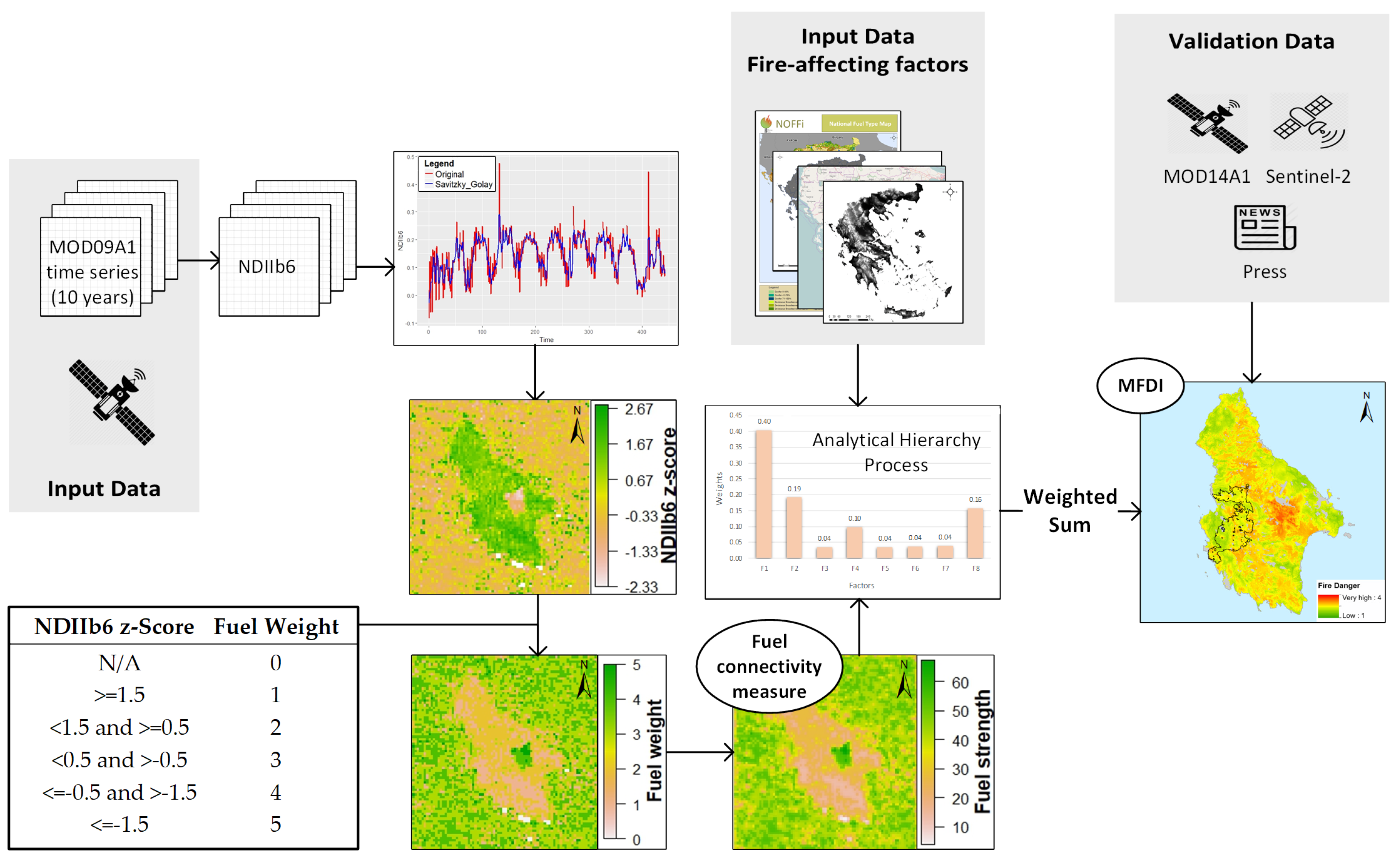
Figure 2 presents the MFDI maps of the four aforementioned test cases, calculated for the eight-day period that each fire erupted.

In Attica (Figure 2a), the mean MFDI value within the burned area is approximately $2.7$. The index presents moderate to very high values (that is, greater than 2) in most of the area’s extent, with the very high values located to the northwest side of the fire-affected area. According to press reports, the specific fire ignited at Dervenoxoria Municipality, near the village Stefani, which is located on the northwest side of Mount Parnitha, where the MFDI values were very high (greater than 3).

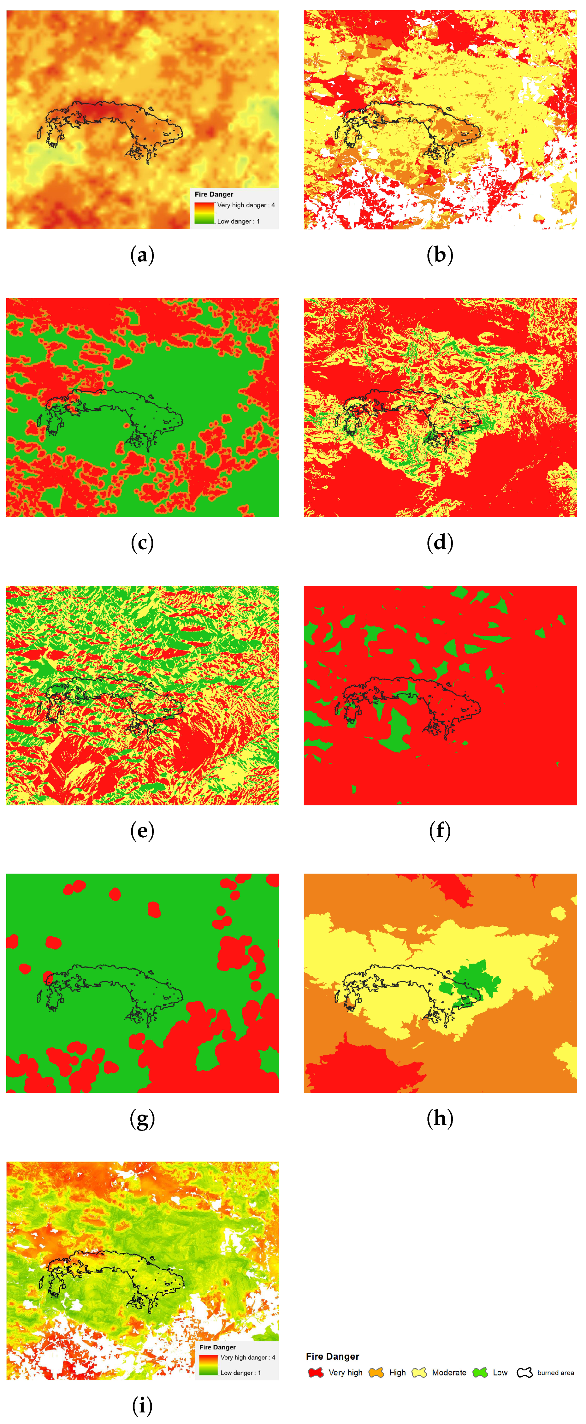
Figure 3 depicts the individual parameters (i.e., input variables) used for the index calculation. We can observe that the fuel connectivity (Figure 3a) exhibits close to maximum values in approximately half the burned area. Although this parameter is assigned the largest (by far) weight by the AHP (see Table 7), most other parameters denote a medium to small danger within most of the burned area. As such, the final result (Figure 3i) reports medium to low risk in most of the affected regions and pinpoints the dangerous areas on the northwestern part of the fire perimeter, where the fire actually started from. This part of the area exhibited high fuel connectivity values, but moreover was surrounded by highly flammable fuels and was close to agricultural and/or urban areas.

The MFDI calculated for Karistos (Figure 2b) exhibits very high danger values (greater than $3.5$) mainly in the northern part of the burned area, whereas the mean index value within the whole fire perimeter is approximately $2.9$. The index validation in this specific case was performed using the MOD14A1 product (Figure 4). More specifically, the region belonging to MOD14A1 pixels of class 9 (fire, high confidence, land or water) within the fire perimeter as compared to the rest of the burned area. The mean MFDI value within the area identified as fire by MOD14A1 (class 9) was $3.4$, i.e., high to very high fire danger. On the other hand, the mean MFDI value of all other pixels within the burned area was $2.8$, i.e., moderate to high fire danger.

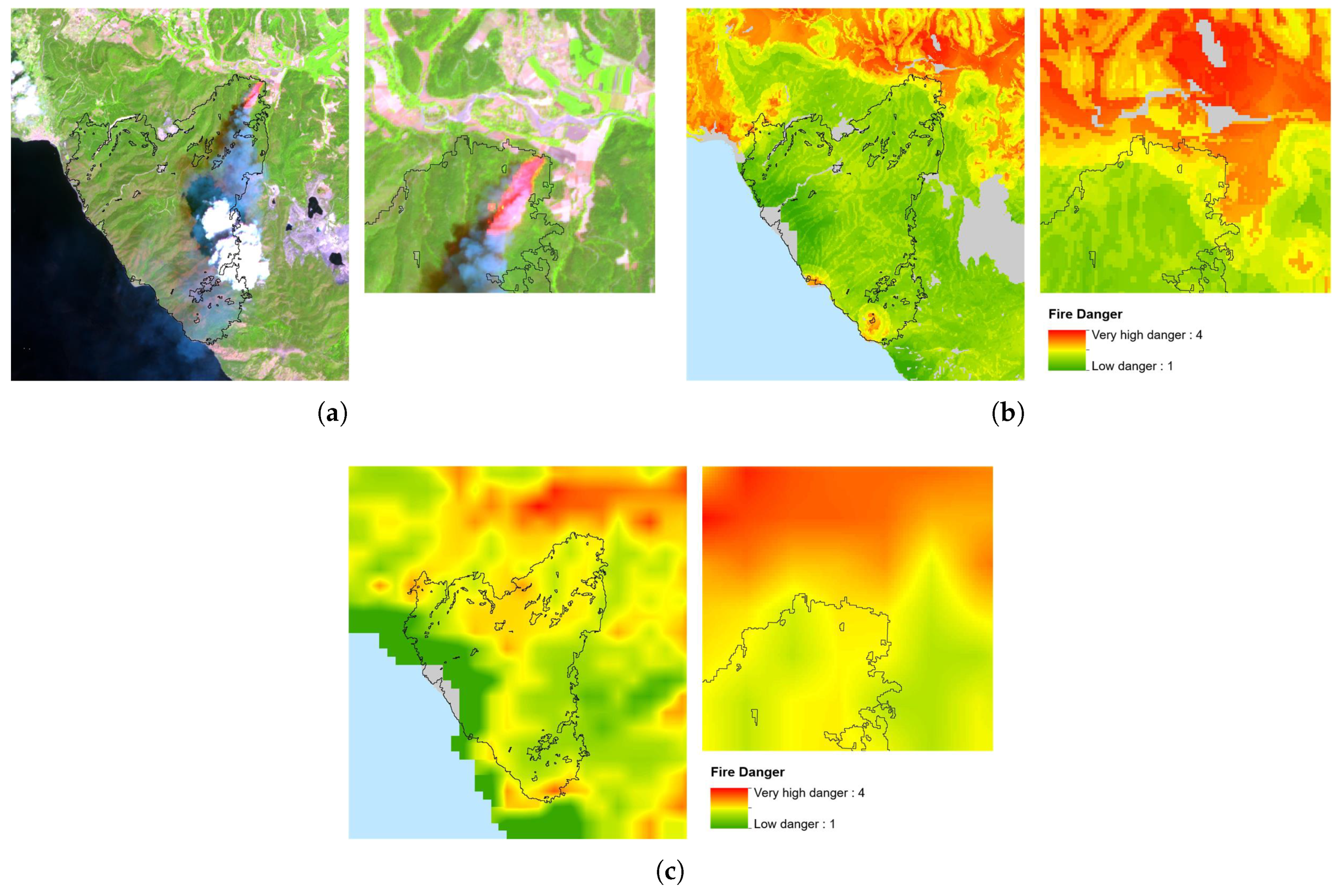
For the Farakla (Euboea region) case (Figure 2c), the index’s accuracy was empirically assessed with the use of a Sentinel-2 satellite image, which was acquired around the time that the fire erupted. The ignition point was located in the northern part of the fire-affected region, which is adjacent to agricultural crops (Figure 5) and characterized by a very high fire danger according to the MFDI map (greater than 3). Indeed, press reports connected the origin of this fire to agricultural burnings. Since the MFDI quantifies the danger for fire ignition and not for spread, high MFDI values are observed only in few areas, one of which is the fire ignition point, contrary to the rest of the burned area. In this case, the strong north wind (clearly identifiable in the Sentinel-2 image from the smoke’s direction) was the reason for the spread of the fire to the south, even though the predicted fire danger was much lower for those areas. Figure 5c depicts the fuel connectivity parameter, which highlights the opposite situation of that observed in Parnitha (Figure 3). In the latter, the high fuel connectivity values within most of the burned area were confined by the other parameters in the final MFDI. Here, the fuel connectivity is medium to low in almost all burned areas, but specific points are highlighted as highly dangerous in MFDI due to their proximity to agricultural areas.

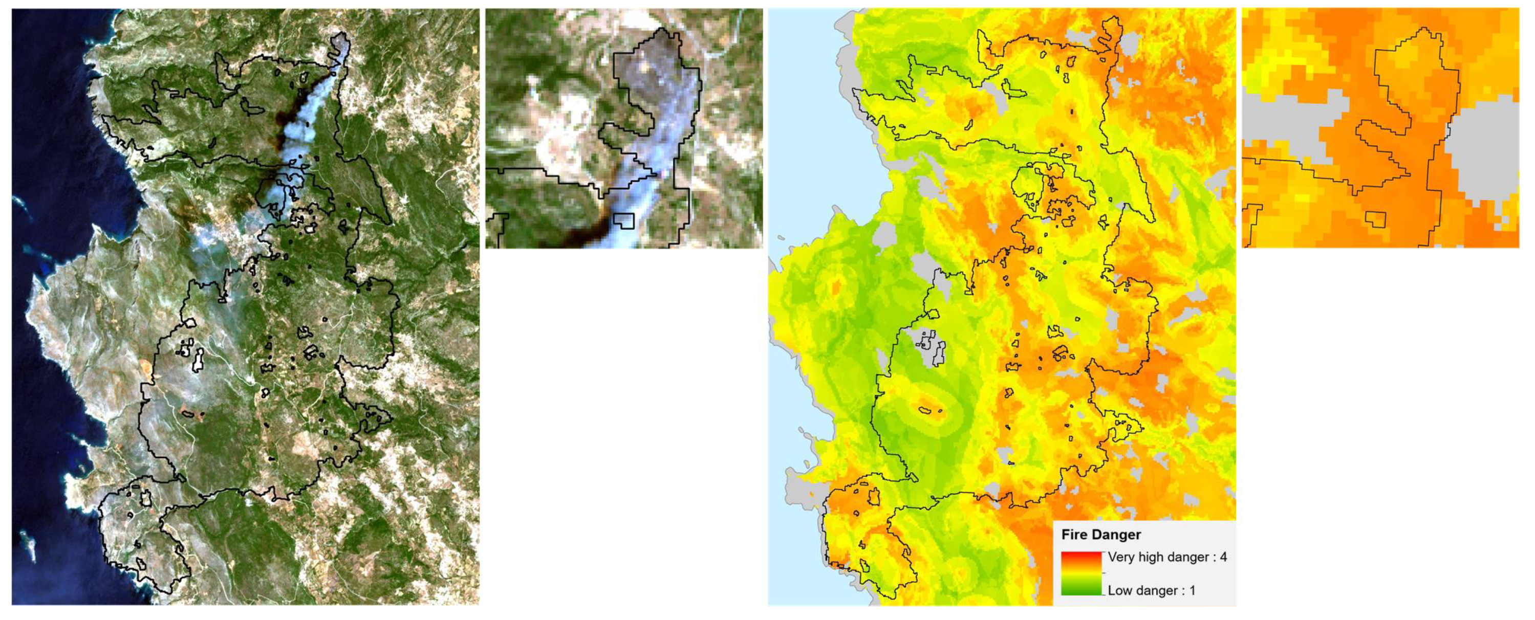
A Sentinel-2 image acquired around the fire eruption time was also used for the validation of the MFDI for the Kythira Island wildfire (Figure 2d). A closer examination of the index values within the burned area (Figure 6) reveals that the fire started in an area where the MFDI exhibited relatively higher values (approximately 3) due to the adjacent of agricultural fields. According to unconfirmed reports, the fire might have started from anthropogenic causes rather than natural ones. This is the reason why most of the fire-affected region comprises low to moderate MFDI values. The presence of intense north winds caused the fire to spread fast and destroy a large forested area.

4. Discussion

The MODIS-derived dry fuel connectivity parameter within the proposed MFDI is used as an indicator of fuel dryness (more precisely, its relative deviation from its historical assumed norm). Since fuel dryness significantly increases fire ignition risk, this parameter was assigned the highest importance among all factors (see Table 7). However, fuel dryness does not only affect fire ignition danger but also the fire spread risk. Therefore, MFDI introduces a number of other parameters, in order to tilt the scale towards the fire ignition danger component rather than the spread risk one. This is evident from the presentation of all individual parameters in the case of the Parnitha wildfire (Figure 3). There, the dry fuel connectivity parameter exhibited high values in almost all the areas burned, but the MFDI values are decreased in most regions by the other factors, with high values being maintained only in some small regions, in one of which the fire actually started from. Conversely, in the Farakla wildfire (Figure 5), the fuel connectivity was medium to low in almost all burned areas, but the ignition point was ultimately highlighted with high MFDI values due to its proximity to agricultural areas. In either case, it is evident that the fuel connectivity measure is not sufficient to quantify the fire ignition danger by itself, which concurs with the empirical observation that a high dryness deviation is an important but not decisive factor for a wildfire to erupt.

It is undeniable that a larger database of fire ignition points is essential for performing a rigorous quantitative assessment of the proposed MFDI, which we are currently pursuing. Lacking such data presently, we reported here all cases for which we could find trustworthy information on the fire ignition locations, either through MODIS data, Sentinel-2 imagery, or cross-checked media information. Even though there are only four test cases, we argue that the results showcase the strong potential of the proposed method in deriving reliable estimations of fire danger, at the very least for the Mediterranean ecosystem of Greece.

The proposed MFDI relies on MODIS-derived NDIIb6 anomaly data (the dry fuel connectivity measure) for identifying abnormal vegetation dryness in the previous eight days the index provides estimation for. The latter is expected to increase fuel flammability potential and, therefore, fire ignition danger in the next eight-days period (for which the index is calculated for), provided that the weather conditions do not change abruptly (i.e., heavy rainfall or otherwise increased humidity). Relying on such a satellite-derived proxy of vegetation dryness allows us to avoid using meteorological data (either measurements or predictions), which exhibit the limitations described in the introduction (e.g., ineffective spatial interpolation if no dense network of meteorological stations exists) and may involve substantial costs for obtaining them. However, weather-based fire danger indices do exhibit advantages compared to our approach, such as the estimation of surface fuel humidity or the prediction of future weather conditions (e.g., precipitation probability, wind intensity, or increased lightning activity that is a frequent source of ignitions, especially in remote forested areas). Therefore, MFDI should be considered as a complementary rather than competitive (to weather-based indices) tool in prefire management. Combining MFDI with weather-based indices or otherwise incorporating meteorological information into the index would be of high interest, but this is a future work outside the scope of the current study.

Accordingly, the other factors—save the fuel dryness—incorporated into MFDI try to capture the most frequent causes of wildfire ignition, but not all. Specifically, fuel type and topographic features cover the most important natural causes of fire ignition. The proximity to agricultural areas, roads, and urban areas was introduced to cover the most frequent anthropogenic sources of fire occurrence, which are mostly due to negligence. Arsons are thus not covered, which is a parameter difficult to model and an open research topic. Incorporating recent research outcomes in this direction in the future would also be very interesting.

5. Conclusions

This paper presented a new method for the reliable estimation of fire ignition danger on a midterm basis. The developed MFDI provides 500m spatial information related to the danger of fire ignition for the next eight days. Its development is primarily based on the availability of satellite data, namely the MODIS eight-day composite products, contrary to other operationally used fire danger indices (for example, the daily index provided by the European Forest Fire Information System—EFFIS), which rely mostly on meteorological predictions. In particular, the proposed method employs MODIS time-series for the spatial estimation of the dry fuel connectivity, which is then combined with ancillary data through a multi-criteria analysis for the derivation of MFDI fire ignition danger estimate.

The index was validated considering the cases of four large wildfires in Greece, namely, the Attica region, the Farakla and Karistos areas at Euboea and the Kythira Island. The validation of the resulting fire danger maps was based on historical fire events and—although not fully quantitative—it showcased that the MFDI may constitute a reliable index for assessing the spatial distribution of wildfire danger. Future investigation of the potential of MFDI in combination with other fire danger indices would be of high interest, in order to effectively support midterm fire prevention planning.

References

1. Khabarov, N.; Krasovskii, A.; Obersteiner, M.; Swart, R.; Dosio, A.; San-Miguel-Ayanz, J.; Durrant, T.; Camia, A.; Migliavacca, M. Forest fires and adaptation options in Europe. Reg. Environ. Chang. 2016, 16, 21–30. [Google Scholar] [CrossRef]
2. Turco, M.; Hardenberg, J.V.; AghaKouchak, A.; Llasat, M.C.; Provenzale, A.; Trigo, R.M. On the key role of droughts in the dynamics of summer fires in Mediterranean Europe. Sci. Rep. 2017, 7, 81. [Google Scholar] [CrossRef] [PubMed]
3. San-Miguel-Ayanz, J.; Moreno, J.M.; Camia, A. Analysis of large fires in European Mediterranean landscapes: lessons learned and perspectives. For. Ecol. Manag. 2013, 294, 11–22. [Google Scholar] [CrossRef]
4. Pereira, M.G.; Hayes, J.P.; Miller, C.; Orenstein, D.E. Fire on the hills: An environmental history of fires and fire policy in Mediterranean-type ecosystems. In Environmental History in the Making; Springer: Berlin/Heidelberg, Germany, 2017; pp. 145–169. [Google Scholar]
5. Füssel, H.M.; Jol, A.; Marx, A.; Hildén, M.; Aparicio, A.; Bastrup-Birk, A.; Bigano, A.; Castellari, S.; Erhard, M.; Georgi, B. Climate Change, Impacts and Vulnerability in Europe 2016-An Indicator-Based Report; European Environment Agency: Copenhagen, Denmark, 2017. [Google Scholar]
6. San-Miguel-Ayanz, J.; Durrant, T.; Boca, R.; Libertà, G.; Branco, A.; de Rigo, D.; Ferrari, D.; Maianti, P.; Artés Vivancos, T.; Schulte, E.; et al. Forest Fires in Europe, Middle East and North Africa 2016; Technical Report EUR 28707 EN; Joint Research Centre, Publications Office: Luxembourg, 2017. [Google Scholar]
7. Kalabokidis, K.; Palaiologou, P.; Gerasopoulos, E.; Giannakopoulos, C.; Kostopoulou, E.; Zerefos, C. Effect of climate change projections on forest fire behavior and values-at-risk in Southwestern Greece. Forests 2015, 6, 2214–2240. [Google Scholar] [CrossRef]
8. Chowdhury, E.H.; Hassan, Q.K. Operational perspective of remote sensing-based forest fire danger forecasting systems. ISPRS J. Photogramm. Remote Sens. 2015, 104, 224–236. [Google Scholar] [CrossRef]
9. Krasnow, K.; Schoennagel, T.; Veblen, T.T. Forest fuel mapping and evaluation of LANDFIRE fuel maps in Boulder County, Colorado, USA. For. Ecol. Manag. 2009, 257, 1603–1612. [Google Scholar] [CrossRef]
10. Jolly, W.M.; Cochrane, M.A.; Freeborn, P.H.; Holden, Z.A.; Brown, T.J.; Williamson, G.J.; Bowman, D.M. Climate-induced variations in global wildfire danger from 1979 to 2013. Nat. Commun. 2015, 6, 7537. [Google Scholar] [CrossRef]
11. Torres, F.; Romeiro, J.; de Albuquerque Santos, A.C.; de Oliveira Neto, R.R.; Lima, G.; Zanuncio, J. Fire danger index efficiency as a function of fuel moisture and fire behavior. Sci. Total Environ. 2018, 631, 1304–1310. [Google Scholar] [CrossRef]
12. Dubé, D.E. The Canadian Forest Fire Danger Rating System: An Overview. For. Chron 1989, 65, 258–265. [Google Scholar]
13. Cohen, J.D.; Deeming, J.E. The National Fire-Danger rating System: Basic Equations; Gen. Tech. Rep. PSW-82; Pacific Southwest Forest and Range Experiment Station, Forest Service, US Department of Agriculture: Berkeley, CA, USA, 1985; 82p.
14. McArthur, A.G. Weather and Grassland fire Behaviour; Forestry and Timber Bureau, Department of National Development, Commonwealth of Australia: Canberra, Australia, 1966.
15. San-Miguel-Ayanz, J.; Carlson, J.D.; Alexander, M.; Tolhurst, K.; Morgan, G.; Sneeuwjagt, R.; Dudley, M. Current methods to assess fire danger potential. In Wildland Fire Danger Estimation and Mapping: The Role of Remote Sensing Data; World Scientific: Singapore, 2003; pp. 21–61. [Google Scholar]
16. Di Giuseppe, F.; Pappenberger, F.; Wetterhall, F.; Krzeminski, B.; Camia, A.; Libertá, G.; San Miguel, J. The Potential Predictability of Fire Danger Provided by Numerical Weather Prediction. J. Appl. Meteor. Climatol. 2016, 55, 2469–2491. [Google Scholar] [CrossRef]
17. Mirto, M.; Mariello, A.; Nuzzo, A.; Mancini, M.; Raolil, A.; Marra, O.; Fiore, S.; Sirca, C.; Salis, M.; Bacciu, V. The OFIDIA Fire Danger Rating System. In Proceedings of the 2015 10th International Conference on P2P, Parallel, Grid, Cloud and Internet Computing (3PGCIC), Krakow, Poland, 4–6 November 2015; pp. 695–700. [Google Scholar]
18. Pinto, M.M.; DaCamara, C.C.; Trigo, I.F.; Trigo, R.M.; Turkman, K.F. Fire danger rating over Mediterranean Europe based on fire radiative power derived from Meteosat. Nat. Hazards Earth Syst. Sci. 2018, 18, 515–529. [Google Scholar] [CrossRef]
19. Horel, J.D.; Ziel, R.; Galli, C.; Pechmann, J.; Dong, X. An evaluation of fire danger and behaviour indices in the Great Lakes Region calculated from station and gridded weather information. Int. J. Wildland Fire 2014, 23, 202. [Google Scholar] [CrossRef]
20. de Jong, M.C.; Wooster, M.J.; McCall, F.F. Calibration and evaluation of the Canadian Forest Fire Weather Index (FWI) System for improved wildland fire danger rating in the United Kingdom. Nat. Hazards Earth Syst. Sci. 2016, 16, 1217. [Google Scholar] [CrossRef]
21. Beccari, A.; Borgoni, R.; Cazzuli, O.; Grimaldelli, R. Use and performance of the Forest Fire Weather Index to model the risk of wildfire occurrence in the Alpine region. Environ. Plan. B Plan. Des. 2016, 43, 772–790. [Google Scholar] [CrossRef]
22. Sharples, J.J.; McRae, R.H.D.; Weber, R.O.; Gill, A.M. A simple index for assessing fire danger rating. Environ. Model. Softw. 2009, 24, 764–774. [Google Scholar] [CrossRef]
23. Bellis, L.; Veronica, A.; Andres, L.; Juan, P.; Sofia, L.; Clemoveki, K.; Scavuzzo, C. Design and implementation of an operational meteo fire risk forecast based on open source geospatial technology. In Proceedings of the 2015 IEEE International Geoscience and Remote Sensing Symposium (IGARSS), Milan, Italy, 26–31 July 2015; pp. 2155–2158. [Google Scholar] [CrossRef]
24. Liu, D.; Zhang, Y. Research of regional forest fire prediction method based on multivariate linear regression. Analysis 2015, 9, 13–22. [Google Scholar] [CrossRef]
25. Knorr, W.; Pytharoulis, I.; Petropoulos, G.P.; Gobron, N. Combined use of weather forecasting and satellite remote sensing information for fire risk, fire and fire impact monitoring. Comput. Ecol. Softw. 2011, 1, 112. [Google Scholar]
26. Mitri, G.; Saba, S.; Nader, M.; McWethy, D. Developing Lebanon’s fire danger forecast. Int. J. Disaster Risk Reduct. 2017, 24, 332–339. [Google Scholar] [CrossRef]
27. Kv, S.B.; Roy, A. Forest fire danger index based on modifying Nesterov Index, fuel, and anthropogenic activities using MODIS TERRA, AQUA and TRMM satellite datasets. In Proceedings of the SPIE 9877, Land Surface and Cryosphere Remote Sensing III, New Delhi, India, 5 May 2016; Khanbilvardi, R., Ganju, A., Rajawat, A.S., Chen, J.M., Eds.; p. 98771A. [Google Scholar] [CrossRef]
28. Caccamo, G.; Chisholm, L.A.; Bradstock, R.A.; Puotinen, M.L. Assessing the sensitivity of MODIS to monitor drought in high biomass ecosystems. Remote Sens. Environ. 2011, 115, 2626–2639. [Google Scholar] [CrossRef]
29. Mosammam, A.M. Geostatistics: Modeling Spatial Uncertainty; Taylor & Francis: Abingdon-on-Thames, UK, 2013. [Google Scholar]
30. Han, K.S.; Viau, A.A.; Anctil, F. High-resolution forest fire weather index computations using satellite remote sensing. Can. J. For. Res. 2003, 33, 1134–1143. [Google Scholar] [CrossRef]
31. Ashcroft, M.B.; Chisholm, L.A.; French, K.O. Climate change at the landscape scale: Predicting fine-grained spatial heterogeneity in warming and potential refugia for vegetation. Glob. Chang. Biol. 2009, 15, 656–667. [Google Scholar] [CrossRef]
32. Leblon, B. Using remote sensing for fire danger monitoring. Nat. Hazards 2005, 35, 343–359. [Google Scholar] [CrossRef]
33. Wang, L.; Hunt, E.R., Jr.; Qu, J.J.; Hao, X.; Daughtry, C.S. Remote sensing of fuel moisture content from ratios of narrow-band vegetation water and dry-matter indices. Remote Sens. Environ. 2013, 129, 103–110. [Google Scholar] [CrossRef]
34. Chowdhury, E.H.; Hassan, Q.K. Development of a new daily-scale forest fire danger forecasting system using remote sensing data. Remote Sens. 2015, 7, 2431–2448. [Google Scholar] [CrossRef]
35. Vermote, E.F.; Kotchenova, S.Y. MOD09 User’s Guide (J/OL); 2008. Available online: https://modis.gsfc.nasa.gov/data/dataprod/mod09.php (accessed on 14 June 2018).
36. Tompoulidou, M.; Stefanidou, A.; Grigoriadis, D.; Dragozi, E.; Stavrakoudis, D.; Gitas, I.Z. The Greek National Observatory of Forest Fires (NOFFi). In Proceedings of the Fourth International Conference on Remote Sensing and Geoinformation of the Environment (RSCy2016), Paphos, Cyprus, 4–8 April 2016; International Society for Optics and Photonics: The Hague, The Netherlands, 2016; Volume 9688, p. 96880. [Google Scholar]
37. Yu, B.; Chen, F.; Li, B.; Wang, L.; Wu, M. Fire Risk Prediction Using Remote Sensed Products: A Case of Cambodia. Photogramm. Eng. Remote Sens. 2017, 83, 19–25. [Google Scholar] [CrossRef]
38. Mitri, G.; Jazi, M.; McWethy, D. Assessment of wildfire risk in lebanon using geographic object-based image analysis. Photogramm. Eng. Remote Sens. 2015, 81, 499–506. [Google Scholar] [CrossRef]
39. Fick, S.E.; Hijmans, R.J. WorldClim 2: New 1-km spatial resolution climate surfaces for global land areas. Int. J. Climatol. 2017, 37, 4302–4315. [Google Scholar] [CrossRef]
40. Satir, O.; Berberoglu, S.; Donmez, C. Mapping regional forest fire probability using artificial neural network model in a Mediterranean forest ecosystem. Geomat. Nat. Hazards Risk 2016, 7, 1645–1658. [Google Scholar] [CrossRef]
41. DaCamara, C.C.; Calado, T.J.; Ermida, S.L.; Trigo, I.F.; Amraoui, M.; Turkman, K.F. Calibration of the Fire Weather Index over Mediterranean Europe based on fire activity retrieved from MSG satellite imagery. Int. J. Wildland Fire 2014, 23, 945. [Google Scholar] [CrossRef]
42. Trigo, I.F.; Dacamara, C.C.; Viterbo, P.; Roujean, J.L.; Olesen, F.; Barroso, C.; Camacho-de Coca, F.; Carrer, D.; Freitas, S.C.; García-Haro, J.; et al. The Satellite Application Facility for Land Surface Analysis. Int. J. Remote Sens. 2011, 32, 2725–2744. [Google Scholar] [CrossRef]
43. Abdollahi, M.; Islam, T.; Gupta, A.; Hassan, Q. An Advanced Forest Fire Danger Forecasting System: Integration of Remote Sensing and Historical Sources of Ignition Data. Remote Sens. 2018, 10, 923. [Google Scholar] [CrossRef] [Green Version]
44. Arganaraz, J.P.; Landi, M.A.; Bravo, S.J.; Gavier-Pizarro, G.I.; Scavuzzo, C.M.; Bellis, L.M. Estimation of Live Fuel Moisture Content From MODIS Images for Fire Danger Assessment in Southern Gran Chaco. IEEE J. Sel. Top. Appl. Earth Obs. Remote Sens. 2016, 9, 5339–5349. [Google Scholar] [CrossRef]
45. Matin, M.A.; Chitale, V.S.; Murthy, M.S.R.; Uddin, K.; Bajracharya, B.; Pradhan, S. Understanding forest fire patterns and risk in Nepal using remote sensing, geographic information system and historical fire data. Int. J. Wildland Fire 2017, 26, 276–286. [Google Scholar] [CrossRef] [Green Version]
46. Babu, K.S.; Roy, A.; Prasad, P.R. Developing the static fire danger index using geospatial technology. In Proceedings of the 2016 2nd International Conference on Contemporary Computing and Informatics (IC3I), Noida, India, 14–17 December 2016; pp. 558–563. [Google Scholar]
47. Babu, K.; Kabdulova, G.; Kabzhanova, G. Developing the Forest Fire Danger Index for the Country Kazakhstan by Using Geospatial Techniques. J. Environ. Informatics Lett. 2019, 1. [Google Scholar] [CrossRef] [Green Version]
48. Liu, W.; Wang, S.; Zhou, Y.; Wang, L.; Zhu, J.; Wang, F. Lightning-caused forest fire risk rating assessment based on case-based reasoning: A case study in DaXingAn Mountains of China. Nat. Hazards 2016, 81, 347–363. [Google Scholar] [CrossRef]
49. Bisquert, M.; Caselles, E.; Sánchez, J.M.; Caselles, V. Application of artificial neural networks and logistic regression to the prediction of forest fire danger in Galicia using MODIS data. Int. J. Wildland Fire 2012, 21, 1025. [Google Scholar] [CrossRef]
50. Akther, M.S.; Hassan, Q.K. Remote sensing-based assessment of fire danger conditions over boreal forest. IEEE J. Sel. Top. Appl. Earth Obs. Remote Sens. 2011, 4, 992–999. [Google Scholar] [CrossRef]
51. Ahmed, M.R.; Hassan, Q.K.; Abdollahi, M.; Gupta, A. Introducing a New Remote Sensing-Based Model for Forecasting Forest Fire Danger Conditions at a Four-Day Scale. Remote Sens. 2019, 11, 2101. [Google Scholar] [CrossRef] [Green Version]
52. Caccamo, G.; Chisholm, L.A.; Bradstock, R.A.; Puotinen, M.L. Using remotely-sensed fuel connectivity patterns as a tool for fire danger monitoring. Geophys. Res. Lett. 2012, 39. [Google Scholar] [CrossRef] [Green Version]
53. Chrysafis, I.; Mallinis, G.; Gitas, I.; Tsakiri-Strati, M. Estimating Mediterranean forest parameters using multi seasonal Landsat 8 OLI imagery and an ensemble learning method. Remote Sens. Environ. 2017, 199, 154–166. [Google Scholar] [CrossRef]
54. Saaty, T.L. A scaling method for priorities in hierarchical structures. J. Math. Psychol. 1977, 15, 234–281. [Google Scholar] [CrossRef]
55. Blaschke, T. Object based image analysis for remote sensing. ISPRS J. Photogramm. Remote Sens. 2010, 65, 2–16. [Google Scholar] [CrossRef] [Green Version]
56. Giglio, L. MODIS Collection 6 Active Fire Product User’s Guide, Revision A; Technical Report; University of Maryland: College Park, MD, USA, 2015. [Google Scholar]
57. Drusch, M.; Del Bello, U.; Carlier, S.; Colin, O.; Fernandez, V.; Gascon, F.; Hoersch, B.; Isola, C.; Laberinti, P.; Martimort, P.; et al. Sentinel-2: ESA’s Optical High-Resolution Mission for GMES Operational Services. Remote Sens. Environ. 2012, 120, 25–36. [Google Scholar] [CrossRef]
58. Chuvieco, E.; Riaño, D.; Aguado, I.; Cocero, D. Estimation of fuel moisture content from multitemporal analysis of Landsat Thematic Mapper reflectance data: Applications in fire danger assessment. Int. J. Remote Sens. 2002, 23, 2145–2162. [Google Scholar] [CrossRef]
59. Hunt, E.R., Jr.; Rock, B.N. Detection of changes in leaf water content using near-and middle-infrared reflectances. Remote Sens. Environ. 1989, 30, 43–54. [Google Scholar]
60. HardiskyMA, K. SmartRM. 1983. The influence of soft salinity, growth form, mad leaf moisture on the spectral reflectance of Spartina alterniflora canopies. Photogramm. Eng. Remote Sens. 1983, 49, 77–83. [Google Scholar]
61. Steinier, J.; Termonia, Y.; Deltour, J. Smoothing and differentiation of data by simplified least square procedure. Anal. Chem. 1972, 44, 1906–1909. [Google Scholar] [CrossRef]
62. Liu, W.T.; Juárez, R.N. ENSO drought onset prediction in northeast Brazil using NDVI. Int. J. Remote Sens. 2001, 22, 3483–3501. [Google Scholar] [CrossRef]
63. Saleska, S.R.; Didan, K.; Huete, A.R.; Da Rocha, H.R. Amazon forests green-up during 2005 drought. Science 2007, 318, 612. [Google Scholar] [CrossRef] [Green Version]
64. Gonzalez, J.R.; del Barrio, G.; Duguy, B. Assessing functional landscape connectivity for disturbance propagation on regional scales-A cost-surface model approach applied to surface fire spread. Ecol. Modell. 2008, 211, 121–141. [Google Scholar] [CrossRef]
65. Saaty, T.L.; Vargas, L.G. Prediction, Projection and Forecasting: Applications of the Analytic Hierarchy Process in Economics, Finance, Politics, Games and Sports; Springer: Dordrecht, The Netherlands, 1991. [Google Scholar]
66. Mu, E.; Pereyra-Rojas, M. Understanding the Analytic Hierarchy Process. In Practical Decision Making; Springer International Publishing: Cham, Switzerland, 2017; pp. 7–22. [Google Scholar] [CrossRef]
67. Saaty, R.W. The analytic hierarchy process—What it is and how it is used. Math. Model. 1987, 9, 161–176. [Google Scholar] [CrossRef] [Green Version]
68. Wedley, W.C. Consistency prediction for incomplete AHP matrices. Math. Comput. Model. 1993, 1, 151–161. [Google Scholar] [CrossRef]
69. Byun, D.H. The AHP approach for selecting an automobile purchase model. Inf. Manag. 2001, 38, 289–297. [Google Scholar] [CrossRef]
70. Dolan, J.G. Shared decision-making—Transferring research into practice: The Analytic Hierarchy Process (AHP). Patient Educ. Couns. 2008, 73, 418–425. [Google Scholar] [CrossRef] [Green Version]
71. Pauer, F.; Schmidt, K.; Babac, A.; Damm, K.; Frank, M.; von der Schulenburg, J.M.G. Comparison of different approaches applied in Analytic Hierarchy Process—An example of information needs of patients with rare diseases. BMC Med. Inform. Decis. Mak. 2016, 16, 117. [Google Scholar] [CrossRef] [Green Version]
72. Ganteaume, A.; Camia, A.; Jappiot, M.; San-Miguel-Ayanz, J.; Long-Fournel, M.; Lampin, C. A Review of the Main Driving Factors of Forest Fire Ignition Over Europe. Environ. Manag. 2013, 51, 651–662. [Google Scholar] [CrossRef] [Green Version]
73. Rego, F.C.; Silva, J.S. Wildfires and landscape dynamics in Portugal: A regional assessment and global implications. In Forest Landscapes and Global Change: Challenges for Research and Management; Azevedo, J.C., Perera, A.H., Pinto, M.A., Eds.; Springer: New York, NY, USA, 2014; pp. 51–73. [Google Scholar] [CrossRef]
74. Babu, S.; Roy, A.; Prasad, P.R. Forest fire risk modeling in Uttarakhand Himalaya using TERRA satellite datasets. Eur. J. Remote Sens. 2016, 49, 381–395. [Google Scholar] [CrossRef] [Green Version]
75. Chuvieco, E.; Congalton, R.G. Application of remote sensing and geographic information systems to forest fire hazard mapping. Remote Sens. Environ. 1989, 29, 147–159. [Google Scholar] [CrossRef]
76. Setiawan, I.; Mahmud, A.R.; Mansor, S.; Mohamed Shariff, A.R.; Nuruddin, A.A. GIS-grid-based and multi-criteria analysis for identifying and mapping peat swamp forest fire hazard in Pahang, Malaysia. Disaster Prev. Manag. Int. J. 2004, 13, 379–386. [Google Scholar] [CrossRef]
77. Vasilakos, C.; Kalabokidis, K.; Hatzopoulos, J.; Kallos, G.; Matsinos, Y. Integrating new methods and tools in fire danger rating. Int. J. Wildland Fire 2007, 16, 306–316. [Google Scholar] [CrossRef]
78. Oliveira, S.; Moreira, F.; Boca, R.; San-Miguel-Ayanz, J.; Pereira, J.M.C. Assessment of fire selectivity in relation to land cover and topography: A comparison between Southern European countries. Int. J. Wildland Fire 2014, 23, 620–630. [Google Scholar] [CrossRef]
79. Guglietta, D.; Migliozzi, A.; Ricotta, C. A Multivariate Approach for Mapping Fire Ignition Risk: The Example of the National Park of Cilento (Southern Italy). Environ. Manag. 2015, 56, 157–164. [Google Scholar] [CrossRef] [PubMed]
80. Calviño-Cancela, M.; Chas-Amil, M.L.; García-Martínez, E.D.; Touza, J. Wildfire risk associated with different vegetation types within and outside wildland-urban interfaces. For. Ecol. Manag. 2016, 372, 1–9. [Google Scholar] [CrossRef] [Green Version]
81. Catry, F.X.; Rego, F.C.; Bação, F.L.; Moreira, F. Modeling and mapping wildfire ignition risk in Portugal. Int. J. Wildland Fire 2010, 18, 921–931. [Google Scholar] [CrossRef] [Green Version]
82. Moreira, F.; Viedma, O.; Arianoutsou, M.; Curt, T.; Koutsias, N.; Rigolot, E.; Barbati, A.; Corona, P.; Vaz, P.; Xanthopoulos, G.; et al. Landscape—Wildfire interactions in southern Europe: Implications for landscape management. J. Environ. Manag. 2011, 92, 2389–2402. [Google Scholar] [CrossRef] [Green Version]
83. De Vasconcelos, M.; Silva, S.; Tomé, M.; Alvim, M.; Pereira, J. Spatial prediction of fire ignition probabilities: Comparing logistic regression and neural networks. Photogramm. Eng. Remote Sens. 2001, 67, 73–81. [Google Scholar]
84. Holland, P.G.; Steyn, D.G. Vegetational Responses to Latitudinal Variations in Slope Angle and Aspect. J. Biogeogr. 1975, 2, 179–183. [Google Scholar] [CrossRef]
85. Mermoz, M.; Kitzberger, T.; Veblen, T.T. Landscape Influences on Occurrence and Spread of Wildfires in Patagonian Forests and Shrublands. Ecology 2005, 86, 2705–2715. [Google Scholar] [CrossRef] [Green Version]
86. Heyerdahl, E.K.; Brubaker, L.B.; Agee, J.K. Spatial Controls of Historical Fire Regimes: A Multiscale Example from the Interior West, Usa. Ecology 2001, 82, 660–678. [Google Scholar] [CrossRef]
87. Romero-Calcerrada, R.; Novillo, C.J.; Millington, J.D.A.; Gomez-Jimenez, I. GIS analysis of spatial patterns of human-caused wildfire ignition risk in the SW of Madrid (Central Spain). Landsc. Ecol. 2008, 23, 341–354. [Google Scholar] [CrossRef]
88. Saglam, B.; Bilgili, E.; Dincdurmaz, B.; Kadiogulari, A.; Küçük, O. Spatio-temporal analysis of forest fire risk and danger using LANDSAT imagery. Sensors 2008, 8, 3970–3987. [Google Scholar] [CrossRef] [PubMed] [Green Version]
Figure 1. Flowchart of the proposed methodology.
Remotesensing 11 02786 g001
Figure 2. MFDI estimated for the fire events of (a) June 2007 at Mount Parnitha (Attica) (b) July 2016 at Karistos (Euboea region), (c) July 2016 at Farakla (Euboea region) and (d) August 2017 at Kithira Island. Green and red colors represent low and very high fire danger, respectively. The polygons with a black outline represent the official perimeters of the burned areas.
Remotesensing 11 02786 g002
Figure 3. The parameters used for the MFDI estimation at Mount Parnitha in Attica (Greece) for the fire event of June 2007 and categorized according to the adopted fire danger classification scheme (1 = low, 2 = moderate, 3 = high, 4 = very high): (a) dry fuel connectivity, (b) fuel types, (c) proximity to agricultural areas, (d) slope, (e) aspect, (f) proximity to road network, (g) proximity to urban areas, (h) elevation, and (i) MFDI.
Remotesensing 11 02786 g003
Figure 4. (a) MFDI and (b) MOD14A1 for the burned area of Karistos (Euboea region).
Remotesensing 11 02786 g004
Figure 5. (a) Zoom of the Sentinel-2 satellite image which depicts the area burned at Farakla (black outlined polygon) on the 30th of July 2016, (b) MFDI for Farakla (black outlined polygon) on the 30th of July 2016, which was estimated for the eight-day period from 27th of July 2016 to 4th of August 2016 (right), (c) Fuel connectivity estimated for Farakla.
Remotesensing 11 02786 g005
Figure 6. (left) Zoom of the Sentinel-2 satellite image that depicts the area burned on the Kythira Island (black outlined polygon) by the fire event of the 4th of August 2017, (right) MFDI estimated on the same area for the eight-day period from the 28th of June 2017 to 5th of August 2017.
Remotesensing 11 02786 g006