Establishment of Plot-Yield Prediction Models in Soybean Breeding Programs Using UAV-Based Hyperspectral Remote Sensing

Abstract

Yield evaluation of breeding lines is the key to successful release of cultivars, which is becoming a serious issue due to soil heterogeneity in enlarged field tests. This study aimed at establishing plot-yield prediction models using unmanned aerial vehicle (UAV)-based hyperspectral remote sensing for yield-selection in large-scale soybean breeding programs. Three sets of soybean breeding lines (1103 in total) were tested in blocks-in-replication experiments for plot yield and canopy spectral reflectance on 454~950 nm bands at different growth stages using a UAV-based hyperspectral spectrometer (Cubert UHD185 Firefly). The four elements for plot-yield prediction model construction were studied respectively and concluded as: the suitable reflectance-sampling unit-size in a plot was its 20%–80% central part; normalized difference vegetation index (NDVI) and ration vegetation index (RVI) were the best combination of vegetation indices; the initial seed-filling stage (R5) was the best for a single stage prediction, while another was the best combination for a two growth-stage prediction; and multi-variate linear regression was suitable for plot-yield prediction. In model establishment for each material-set, a random half was used for modelling and another half for verification. Twenty-one two growth-stage two vegetation-index prediction models were established and compared for their modelling coefficient of determination (R_M²) and root mean square error of the model (RMSE_M), verification R_V² and RMSE_V, and their sum R_S² and RMSE_S. Integrated with the coincidence rate between the model predicted and the practical yield-selection results, the models, M_A1-2, M_A4-2 and M_A6-2, with coincidence rates of 56.8%, 58.5% and 52.4%, respectively, were chosen for yield-prediction in yield-test nurseries. The established model construction elements and methods can be used as local models for pre-harvest yield-selection and post-harvest integrated yield-selection in advanced breeding nurseries as well as yield potential prediction in plant-derived-line nurseries. Furthermore, multiple models can be used jointly for plot-yield prediction in soybean breeding programs.

1. Introduction

In plant-breeding programs, accurate yield evaluation of breeding lines is the key to release of novel cultivars since yield is always the most important trait among those targeted [1,2]. In conventional breeding processes, two major links are involved, one is derivation of breeding populations with targeted variants through hybridization and/or mutagenesis, the other is selection for the targeted variants through successive field tests integrated with some necessary lab evaluations. In the selection step, precise yield evaluation of the variants or breeding lines mainly depends on precise field experiments, which is often influenced by complicated environmental conditions (mainly soil uniformity) acting on the field plots, especially as the tested number of lines increased. In fact, yield evaluation of breeding lines is the key to successful release of cultivars, which is becoming a serious issue due to soil heterogeneity in enlarged field tests. For raising the experiment precision, a series of experiment designs and corresponding statistical methods were developed in last century, including various incomplete block designs such as blocks in replication design and lattice design which can test hundreds of breeding lines in a same experiment [3]. However, even so, the soil heterogeneity is still difficult to overcome with for a yield test comprising thousands of breeding lines. That requires new techniques to improve the yield-test precision and yield-selection efficiency and effectiveness.

Remote-sensing images have been widely used in the measurement of crop traits, such as plant height, chlorophyll content, leaf area index (LAI), disease susceptibility, drought stress sensitivity, nitrogen content, yield and etc. [4,5,6,7,8,9]. These are based on the differences in spectral reflectance of the canopy among varieties for the above traits [10]. The most of the field-based research for yield estimation models using canopy reflectance and canopy temperature measurements were focused on 2 or 3 band indices, which can be highly variable and inconsistent among breeding lines or varieties [11]. The biophysical/biochemical components of the field population, such as the canopy and leaf structures, may not allow the plant to fully reach its genetic yield potential [4]. Some researchers have suggested that yield gains observed in field crops can be attributed to more efficient photosynthetic parameters in addition to genetic reasons [12,13,14,15]. Studies that focus on utilizing full spectrum instruments in prediction models have been reported in recent years in wheat [16,17,18], corn [19], rice [20], cotton [21] and soybean [22,23] in optimal and/or drought environments.

Hyperspectral remote sensing provides a continuous spectrum with plentiful band information and high-resolution images. Hyperspectral imaging has become a common method used to predict crop traits and yields [24,25]. Hyperspectral remote-sensing data acquired from the ground [26,27,28], unmanned aerial vehicles [10,29,30,31], airborne platforms [32] and satellite platforms [33] can capture crop canopy spectra in narrow bands and thereby provide information on the biophysical/biochemical composition of the canopy. Low-altitude and flexible unmanned aerial vehicles (UAV) provide an important, affordable and low-cost approach to quantify the components of crop phenotyping [34,35] and precision agriculture [36,37]. Therefore, the UAV are becoming critical in high-throughput crop phenotyping of large number of plots and field trials in a near real-time and dynamic way.

In using UAV equipped with an imaging spectrometer, to find band regions that most significantly contribute to yield estimation is the key to the prediction accuracy. Early researches focused on finding new wavelengths and spectral regions that correlated to plant function. Tucker [38] proposed 5 primary and 2 transition regions of the visible and near infrared spectrum to characterize plant functions. Signal-to-noise ratio in remote-sensing research is always a concern, and sensing the reflectance of plant canopies increases this ratio [19]. In addition, not all the hyperspectral reflectance data in a plot, but those from certain sizes of plot can be used to avoid the border influence between plots, thus the optimized sampling area of hyperspectral reflectance in a plot should be identified to minimize the prediction error.

In the study on hyperspectral remote-sensing technology, strategies for high-throughput field-based phenotyping were investigated with different methods, which showed an obvious difference in estimation accuracy. Vegetation indices are used usually to maximize the relationship between certain reflectance wavelengths and plant function when the effect of background noise is well-controlled [39,40]. The most of the vegetation indices correlate with plant parameters such as pigment status, grain yield. OSAVI (optimized soil-adjusted vegetation index), EVI (enhanced vegetation index), RVI (ration vegetation index), PVI (perpendicular vegetation index) and DVI (difference vegetation index) can be used to estimate leaf nitrogen content [8,41], while NDVI (normalized difference vegetation index), RVI and GNDVI (green and near infrared difference vegetation index) have been used extensively to predict yield and other plant functions in many crops using hyperspectral and satellite imagery [42,43,44,45,46,47,48,49,50,51,52,53]. The 10 vegetation indices often used for yield prediction are listed with their full names, formulae and references in

Table 1. The spectral vegetation indices used in the present study.

Vegetation Index	Full Name of Index	Algorithm Formula	Reference
NDVI	Normalized Difference Vegetation Index	(Rx1 − Rx2)/(Rx1 + Rx2)	[57]
RVI	Ratio Vegetation Index	Rx1/Rx2	[58]
VOG1	Vogelmann Red Edge Index 1	R740/R720	[59]
GNDVI	Green Normalized Difference Vegetation Index	(R780 − R550)/(R780 + R550)	[60]
NDVI705	Normalized Difference Vegetation Index705	(R750 − R705)/(R750 + R705)	[61]
PVI	Perpendicular Vegetation Index	(RNIR − aRRed − b)/(1 + a2)	[62]
RDVI	Renormalized Difference Vegetation Index	(R800 − R670)/(R800 + R670)	[63]
OSAVI	Optimized Soil-Adjusted Vegetation Index	(1 + 0.16)(R800 − R670)/(R800 + R670 + 0.16)	[64]
EVI	Enhanced Vegetation Index	2.5(RNIR − R680)/(1 + RNIR + 6R680 − 7.5R460)	[65]
DVI	Difference Vegetation Index	RNIR − RRed	[66]

Note: R_x1 and R_x2 represent hyperspectral reflectance bands in near infrared and visible red region, respectively.R₇₄₀, R₇₂₀, R₇₈₀, etc. represent hyperspectral reflectance of bands at 740, 720 and 780 nm, etc.

. In literature, the yield prediction model that was constructed from NDVI at the flowering, podding, and seed-filling stages of all breeding lines was the best, with a coefficient of determination (R²) value of 0.66 [28]. Sensitive vegetation indices in the form of NDVI and RVI based on canopy spectral reflectance were suggested to predict the grain yield of soybean by Ma et al [45] and Qi [54], where NDVI was found to have the highest correlation with soybean yield.

In our breeding programs in north China, more than 1000 breeding lines are yield-tested usually for cultivar releasing each year. To make a precise yield evaluation and selection, we took incomplete block design (Blocks in Replication design), additional check plots, precise field management and careful plot-yield harvest. But the plot yield of lines were still fluctuated obviously. We considered using UAV-based hyperspectral remote sensing to predict plot-yield of lines as an auxiliary yield selection tool in addition to the above fine experiment procedures. Thus, the present study aimed at to explore how to establish prediction models for plot-yields in breeding programs for soybeans using UAV-based hyperspectral remote sensing, to establish, validate and select optimal plot-yield prediction models, and then to demonstrate their efficiency and effectiveness in real breeding programs. To fulfill the objective, the major elements in model construction, including the optimal plot sizes for a representative reflectance data set, suitable vegetation indices with their optimal spectral bands, appropriate growth stage for hyperspectral remote sensing data collection and appropriate regression models corresponding to the vegetation indices and spectral bands were studied using plot-yield and UAV-remote-sensing data on four sets of large number of breeding lines in a real soybean breeding program. The selected prediction models were examined for utilization in a real breeding program.

2. Materials and Methods

The whole process of the study includes the following five linked steps: (i) four sets of breeding lines in the real breeding programs were tested and UAV remote-sensed; (ii) the optimal plot sizes for representative reflectance data set were determined; (iii) based on the three of four yield-test breeding line data sets, the optimal vegetation indices along with their optimal spectral bands were analyzed and selected (another set of plant-derived-line data was for validation); (iv) a series of regression models using different vegetation indices (and their combinations) extracted from single or multiple stage hyperspectral remote-sensing data were analyzed for their precision; (v) the selected prediction models were examined with the verification root mean square error (RMSE_V) and real breeding selection results. Finally, three best models were selected for yield prediction in 1st- and 2nd-year yield-test as well as for plant-derived-line evaluation which may be used in comprehensive yield selection integrated with the harvested yield records. Please see the flowchart for the UAV data-processing process (Supplementary material Figure S1).

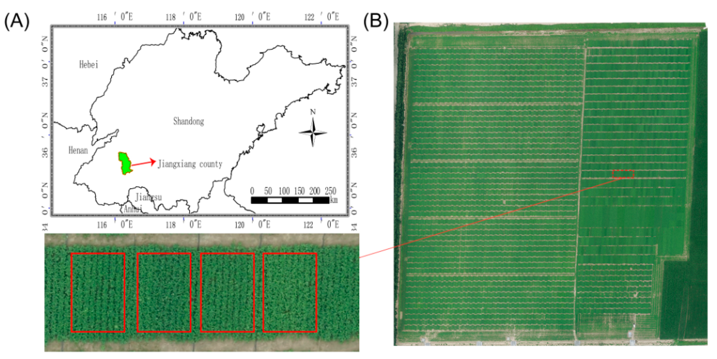
2.1. Plant Materials and Field Experiments

The study was taken along with a real soybean breeding program at Shandong Shofine Seed Technology Co. Ltd. The first-year yield-test in 2015 (1stYYT 2015) with 532 breeding lines, second-year yield-test in 2015 (2ndYYT 2015) with 274 breeding lines, and the second-year yield-test in 2016 (2ndYYT 2016) with 297 breeding lines in a total of 1103 breeding lines were used for establishment and verification of yield prediction models. In addition, a recombinant inbred lines population derived from NN1138-2×KF-1 (named NJRIKY) with 441 lines were used for verification of the prediction models to imitate the selection for plant-derived-line at early breeding stage (Supplementary material Table S1).

The experiments were designed and conducted at Shofine Seed Technology Co. Ltd. in Jining, Shandong, China (E 116°22′10~20″, N 35°25′50″~26′10″) in 2015–2016 as indicated in Table S1 and Figure 1A,B. Each set of lines were tested in a blocks in replication design experiment with three replications using randomized complete blocks design analysis as an approximation [3]. The detailed allocations are listed in Table S1. These breeding lines vary obviously in yield, plant height, growth period, and other agronomic traits. In 2ndYYT 2015, 48 breeding lines were retained in the 2ndYYT 2016, and 165 breeding lines of the 1stYYT 2015 were promoted to the 2ndYYT 2016, these two groups of lines having two years of spectral reflectance and corresponding yield data, therefore, can offer more information for establishing and validation of the prediction models. The planting density was approximately 190,000 plants ha⁻¹. The plot seed yield was measured by harvesting plots with the seed moisture adjusted to 13%, recorded as t ha⁻¹.

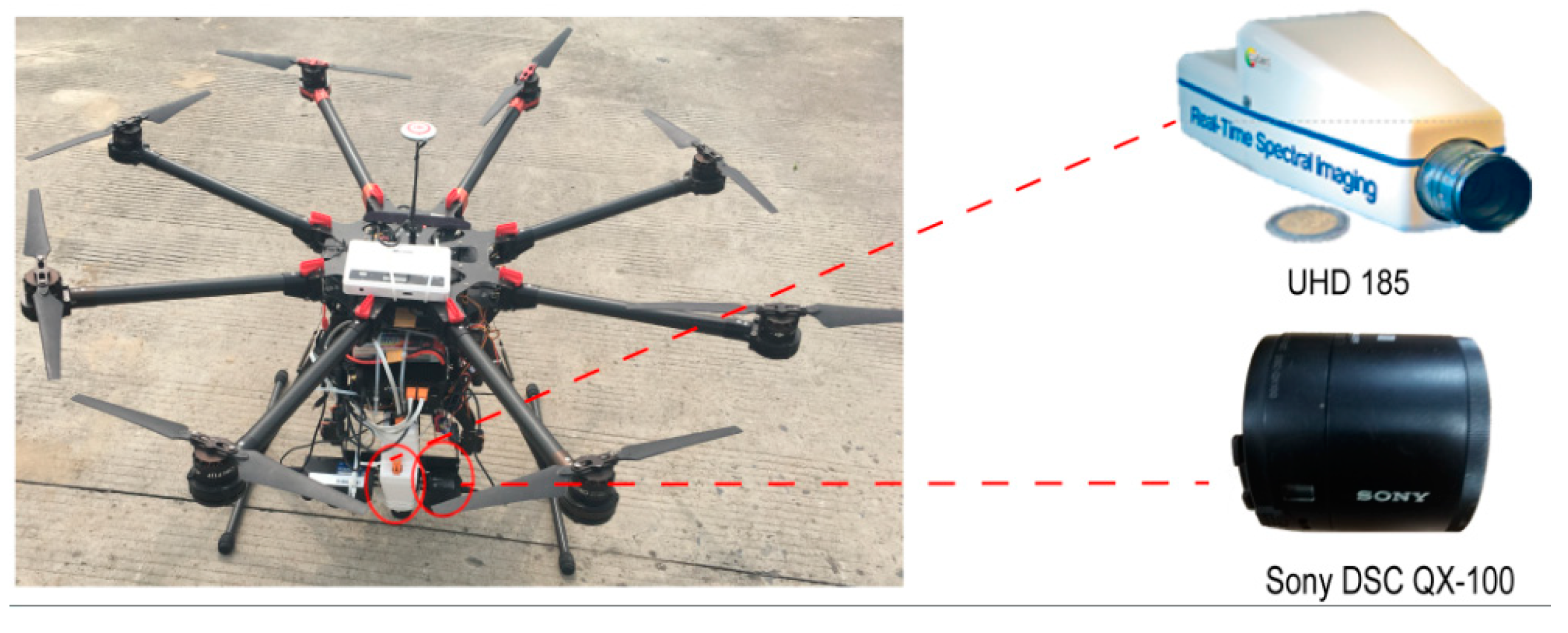
2.2. Assembly of the Unmanned Aerial Vehicle (UAV)-Based Hyperspectral Remote-Sensing System

An UAV with eight rotors, flying height around 50 m, equipped with a Cubert UHD185, a Sony digital camera and a position-orientation system, was assembled for taking the hyperspectral reflectance (Figure 2). The total weight of the attached equipment was approximately 470 g and its housing was measured approximately 28 × 6.5 × 7cm. The instrument had a spectral range of 454 nm to 950 nm, a 4-nm spectral sampling interval, an 8-nm spectral resolution at 532 nm, and a total of 125 spectral channels. For each band, a 50 × 50 pixel image with a 12-bit dynamic range (4,096 digital numbers, DN) was created. Inside the camera, the different bands were projected to different parts of a charged coupled device (CCD). At the same time, as the hyper spectrum (HS) image was being recorded, a grayscale image with a resolution of 990 × 1000 pixels was captured.

Before the UAV flight, de-noising and lens distortion correction were completed. A black and white board was used for radiation calibration of the UHD185 (Table S2). For stitching the hyperspectral image, a certain degree of image was overlapped (heading overlap >70%, side overlap >30%). To obtain stable data, the reflectance was taken on the day with calm and cloudless weather.

2.3. Processing of the UAV Hyperspectral Reflectance and Determination of the Reflectance-Sampling Unit-Size in Plots

The software, Cubert-Pilot (Version1.1, Cubert GmbH, Ulm, Germany) and Agisoft Photoscan Pro (Version 1.4, Agisoft LLC, Russia) were used to realize the image mosaic [55,56]. All graphs of the maximum area vector of each plot were used to fit the ArcGIS software (Version10.0, ESRI, Redlands, USA) on the spliced hyperspectral image. The POS (position and orientation system) data, digital image and hyperspectral data were aligned and fused. DOM (digital orthophoto map) data were obtained after four steps of pre-processing: including (i) aligning photos, (ii) building the dense cloud, (iii) building the mesh, (iv) building the texture. The process of obtaining the UAV hyperspectral reflectance data is shown in Figure S1.

Based on the image mosaic, reflectance-sampling unit-size (area in a testing plot) was studied to avoid the boarder influence. The sample unit was centered on the geometric center of each plot to avoid the space vector region beyond the plot boundary. Then, the bandmath module of ENVI software (Version 4.8, HARRIS geospatial, Wokingham, UK) combined with IDL (Interactive Data Language) was used to scale the length and width of the maximum area of each plot by 20 times (unit-sizes were designed using ENVI procedure, Table S3), and thus, 21 reflectance-sampling unit areas were defined, which were then used as vector images to obtain 21 reflectance-sampling unit data sets. The coefficient of variation (CV) of the top three vegetation indexes (NDVI, RVI and VOGI) were calculated for all the 21 reflectance-sampling units using the analysis of variance (ANOVA) procedure (SAS Institute Inc., NC, USA). Based on the relationship between the CV and reflectance-sampling unit-size, the best unit-size was chosen for further analysis.

2.4. Optimization of the Vegetation Indices along with Corresponding Hyperspectral Bands

All two-band combinations (R(x1) and R(x2)) for the 10 most popular vegetation indices related to yield prediction reported in previous literature, including NDVI, RVI, VOGI (Vogelmann red edge index 1) and others in Table 1, within the spectral range of 454~950 nm, were screened and constructed according to the vegetation index formulas.

The contour map of determination coefficients (R², Equation(1)) was plotted according to the value of R² completed with “plsregress” function in MATLAB R2010b (MathWorks, Inc., Natick, MA, USA). From the contour map, the sensitive wavebands along with the corresponding indices were identified according to their largest R² values. The R² are calculated as follows:

$$R^2=1-\frac{{\sum }_{i=0}^n{(x_i-y_i)}^2}{{\sum }_{i=0}^n{(x_i-\overline{x})}^2}$$

(1)

where x_i and y_i are the measured yield value and the predicted yield value, respectively, $\overline{x}$, is the average value of x_i $i$ varies from 0 to n, where n is the number of tested breeding lines.

2.5. Establishment and Verification of the Yield Prediction Models

In this study, three sets of breeding lines in a total of 1103 (1stYYT 2015, 2ndYYT 2015 and 2ndYYT 2016) were tested for their plot yield and canopy spectral reflectance at the full flowering stage (R2), the full podding stage (R4), the initial seed filling stage (R5), and the full seed filling stage (R6) using a UAV-based hyperspectral spectrometer. The software “plsregress” function in MATLAB R2010b randomly takes half of the lines in each test for establishing the yield prediction model and takes the other half for validation of the established model. The soybean yield prediction models were established from the different material sets based on linear and non-linear (curvilinear) regressions. The formula of the root-mean square-error (RMSE) was used to evaluate the precision of the established models, which is as follows:

$$RMSE=\sqrt{\frac{{\sum }_{i=1}^n{\left(x_i-y_i\right)}^2}{n}}$$

(2)

where x_i and y_i are the measured yield value and the predicted yield value, respectively, $i$ varies from 0 to n while n is the number of tested breeding lines.

The coefficient of determination in model construction is designated as R_M² and the root mean square error of the model as RMSE_M; the coefficient of determination calculated from the other half of the lines is used for validation and designated as R_V² and the root mean square error of the model as RMSE_V; both sets of determination coefficient and root mean square error are used to assess the yield prediction model. For a comprehensive evaluation to balance the modelling and verification, these two parts were summed up as R_S² and RMSE_S. Yield predictions with higher R² and lower RMSE are deemed to be better ones.

All of these statistics (R_M², RMSE_M, R_V², RMSE_V) were completed with MATLAB R2010b software (MathWorks, Inc., Natick, MA, USA). The calibration and validation of the established yield model were calculated by using Microsoft Excel 2007 (Microsoft Corporation, Redmond., Washington, USA).

2.6. Superior Plot-Yield Prediction Models Selected for Breeding Programs

Twofold methods were used to verify all of the established yield prediction models. In the first method, all the models were evaluated with the three sets of yield-tested breeding lines using RMSE_V summed over the three sets of breeding lines. In the second method, in breeders’ actual yield selection, the breeding line with average yield in a single year less than 3.00 t ha⁻¹ is treated as low-yielding line to be eliminated (Eli), that with average yield in a single year more than 3.75 t ha⁻¹ is treated as high-yielding line to be promoted (Pro) and that with average yield in a single year between 3.00 and 3.75 t ha⁻¹ is treated as intermediate line to be reserved for further observation (Res). According to the selection classification, the prediction values of lines in each of the three sets of tests (1stYYT 2015, 2ndYYT 2015 and 2ndYYT 2016) were grouped into the respective categories and compared with the actual selection results. The coincidence rate between the predicted classification and actual breeding classification was calculated for each of the three yield-tests as well as the total value of the three tests.

Based on the results from the two methods, the superior plot-yield prediction models were determined and also were checked for their utilization in plant-derived line selection.

3. Results

3.1. Field Experiment Precision and Variation among the Tested Breeding Lines

The yield distribution, variation, and coefficient of variation (CV) of the four sets of breeding lines are summarized in

Table 2. The frequency distribution of plot yield means averaging over replications in three sets of soybean breeding lines and one set of plant-to-lines tested in 2015–2016.

Material Data Set	Class Limit (t ha−1)										Range (t ha−1)	Mean (t ha−1)	GCV (%)	CV (%)	F-Value
	<2.0	2.0–2.3	2.3–2.6	2.6–2.9	2.9–3.2	3.2–3.5	3.5–3.8	3.8–4.1	>4.1	Σ
1stYYT 2015	6	28	53	59	83	80	86	72	65	532	1.83–4.99	3.32	34.85	19.18	3.30 **
2ndYYT 2015	1	2	17	25	42	44	53	51	39	274	1.65–4.91	3.50	29.35	15.89	3.41 **
2ndYYT 2016	6	9	31	58	80	59	35	16	3	297	1.72–4.41	3.06	26.90	12.81	4.87 **
NJRIKY2015	166	121	101	37	11	5	0	0	0	441	1.08–3.39	2.14	33.15	33.31	0.99 **

Note: ∑: sum; CV: coefficient of variation; GCV: genotypic coefficient of variation; ** indicates significance at 0.01 level. 1stYYT 2015, 2ndYYT 2015, 2ndYYT 2016 and NJRIKY 2015: the first-year yield-test in 2015, the second-year yield-test in 2015, the second-year yield-test in 2016, and the NJRIKY (plant-to-lines population) yield-test in 2015, respectively.

. The average plot seed yield of the breeding lines of the 1stYYT 2015 ranged between 1.83 and 4.99 t ha⁻¹, that of 2ndYYT 2015 ranged from 1.65 to 4.91 t ha⁻¹, that of the 2ndYYT 2016 ranged between 1.72 and 4.41 t ha⁻¹ and the average plot yield of the plant-to-lines of NJRIKY ranged from 1.08 to 3.39 t ha⁻¹, with their genotypic coefficient of variation values of 34.85%, 29.35%, 26.90% and 33.15%, and their error coefficient of variation of 19.18%, 15.89%, 12.81% and 33.31%, respectively. These results indicated that large yield variation existed in the three sets of breeding lines with small experimental errors while there was larger yield variation and experimental error but less mean yield for the NJRIKY plant-derived lines population. Therefore, the data of the three sets of breeding lines were used for the establishment and validation of yield-prediction models from which the established models can fit a relatively wide situation, while those of the NJRIKY was to be used for calibration of the established prediction models to imitate the plant-derived line prediction and selection.

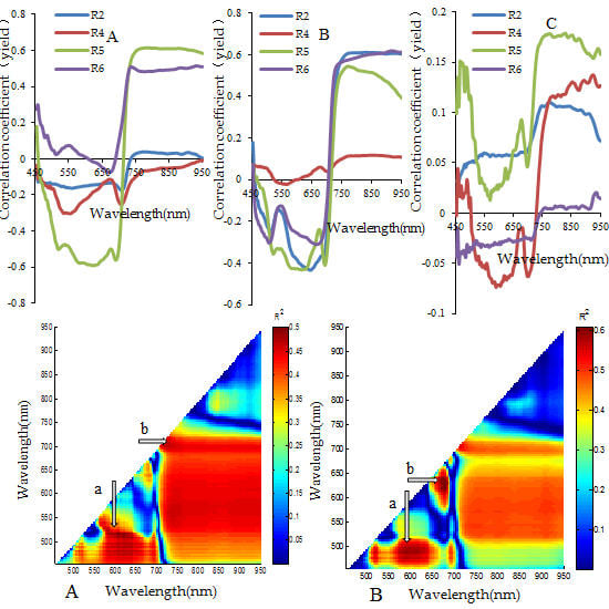
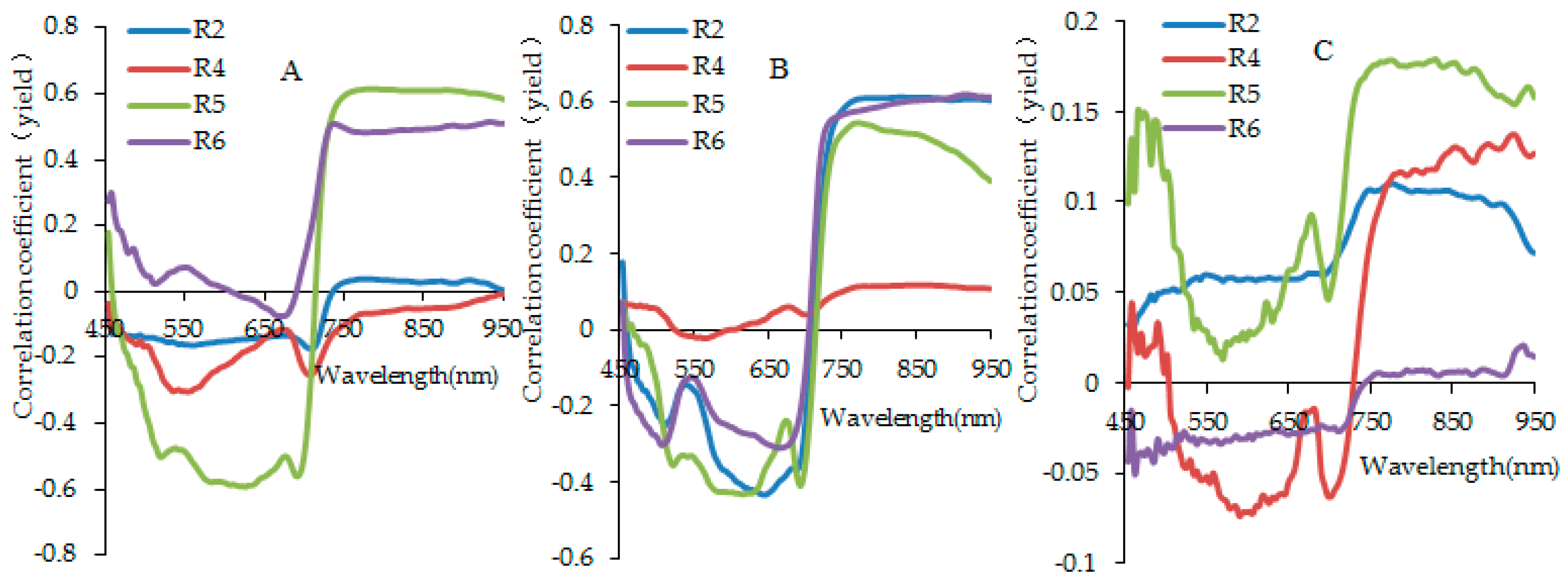
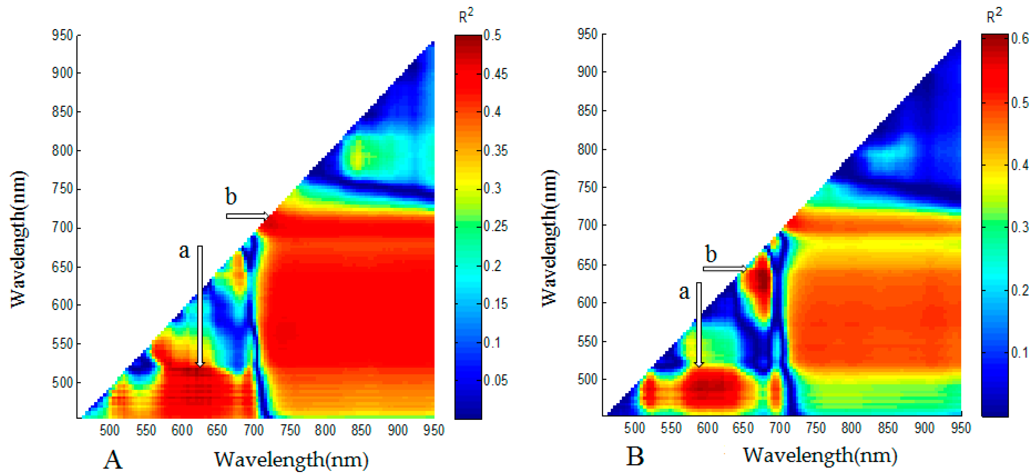
3.2. Analysis for Sensitive Wavebands and Optimal Vegetation Indices for Breeding Line Yield-Prediction

For identifying the hyperspectral reflectance wavebands sensitive to yield, the yield of 2ndYYT 2015 (Figure 3A), 1stYYT 2015 (Figure 3B), NJRIKY test 2015 (Figure 3C) and their corresponding average hyperspectral data at R2, R4, R5 and R6 were analyzed, The wavelengths with maximum and minimum correlation coefficients between spectral reflectance and seed yield were 750~950 nm and 454~710 nm, respectively, for the tests (Figure 3).

Based on the 2ndYYT 2015 (Figure 4A) and 1stYYT 2015 (Figure 4B) data, the contour maps of determination coefficients of linear regression between the two-band NDVI, RVI at R5 stage and yield were established using the “plsregress” function in MATLAB procedure. The dark red area presented the highest correlation zone, and the best sensitive bands for yield-prediction concentrated in the range of 550 nm to 750 nm.

The results of the relationship between vegetation indices and yield at different single growth stages analyzed using MATLAB procedure are listed in

Table 3. The sensitive bands and determination coefficient ranks of the 10 vegetation indices calculated from hyperspectral reflectance and plot yield in two sets of breeding lines yield-tested in 2015.

Item		R2		R4		R5		R6
Breeding line yield-test		1s tYYT	2nd YYT	1s tYYT	2nd YYT	1st YYT	2nd YYT	1st YYT	2nd YYT
Sensitive band (nm)	λ1	750	482	750	514	634	514	550	550
	λ2	770	590	770	606	674	606	710	710
Vegetation index	NDVI	1	1	2	2	2	1	2	2
	RVI	2	2	1	1	1	2	1	1
	GNDVI	4	4	4	4	9	9	3	9
	PVI	5	9	9	10	10	10	10	3
	OSASI	3	7	3	5	4	4	5	4
	EVI	9	10	5	6	7	5	4	6
	RDVI	6	3	6	9	3	8	6	5
	VOG1	8	8	8	8	8	7	7	8
	DVI	10	6	10	3	5	3	9	10
	NDVI705	7	5	7	7	6	6	8	7
Maximum R2		0.58	0.08	0.36	0.19	0.68	0.50	0.54	0.33

Note: λ1 and λ2: two sensitive bands. R2, R4, R5 and R6: growth stages of soybean at the full flowering stage (R2), the full podding stage (R4), the initial seed filling stage (R5), and the full seed filling stage (R6). 1st YYT and 2nd YYT: the first-year yield-test in 2015, the second-year yield-test in 2015.

; the sensitive bands of the 1stYYT 2015 at R2, R4, R5 and R6 growth stages were 750 nm and 770 nm, 750 nm and 770 nm, 634 nm and 674 nm and 550 nm and 710 nm, respectively, while those of the 2ndYYT 2015 were 482 nm and 590 nm, 514 nm and 606 nm, 514 nm and 606 nm and 550 nm and 710 nm, respectively. This indicated that the sensitive bands varied greatly between the two breeding line tests for the same growth stage, while the sensitive bands also varied at the different growth stages even for a same yield-test.

Table 3 also shows that the yields of the two tests were all highly correlated with canopy reflectance at R5 stage, with the maximum R² up to 0.68 and 0.50 respectively, and therefore, the best growth stage to collect the UAV hyperspectral reflectance data for yield-prediction using vegetation indices was at R5, while the spectral sensitive bands for soybean yield-prediction were in 454~850 nm. The other growth stages, R2, R6 and R4, were in turn not as good as R5. The 10 vegetation indices were ranked for each of the growth stages in the two yield-tests according to their determination coefficients, NDVI and RVI were all ranked the top two (Table 3). Since NDVI and RVI based on filtered optimized bands are the two most sensitive indices, they were selected for the establishment of yield-prediction models in this research.

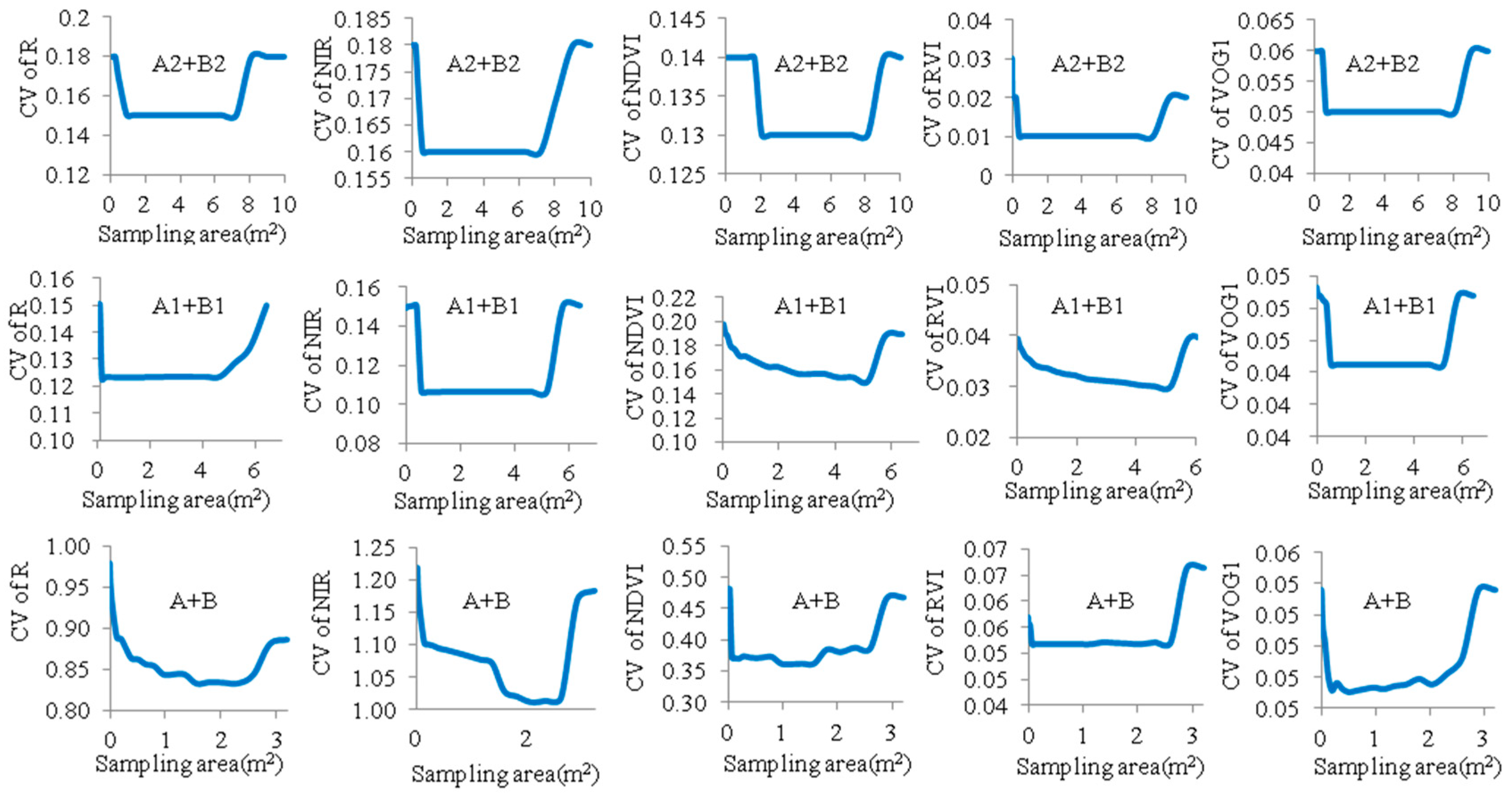
3.3. Optimized Reflectance-Sampling Unit-Size for Organizing the UAV Hyperspectral Reflectance Data

From the UAV reflectance data set of the breeding lines, the hyperspectral data of each plot were obtained using the vector image georeferenced with the hyperspectral image. Twenty-one reflectance-sampling unit-sizes were designed using ENVI procedure combined with IDL language (Table S3), each plot image and vector map at each spatial scale were read, and the 21 datasets of the average spectral reflectance in each plot were extracted (Figure S2). It could be seen that the spectral reflectance of the canopy corresponding to different spatial sampling unit areas was of no significant difference in 550~750 nm of the visible light bands, but the difference was significant in the 750~850 nm near-infrared region. To select the best sampling unit-size of hyperspectral reflectance and eliminate plot marginal effects, the hyperspectral reflectance plot data of 2ndYY T2015, 1stYYT 2015 and NJRIKY at R5 growth stage were used. The CVs of red and near-infrared band, NDVI, RVI and VOG1 of the three tests were also calculated from the spectral information extracted from the 21 different reflectance-sampling unit-sizes. The smaller the value of the coefficient of variation, the better the reflectance-sampling unit-size. Figure 5 showed that the CV of red-band, near-infrared, NDVI, RVI and VOG1 distributed between 0.15~0.18, 0.16~0.18, 0.13~0.14, 0.01~0.02, 0.05~0.06 for 2ndYYT 2015, and 0.12~0.15, 0.11~0.15, 0.15~0.20, 0.03~0.04, 0.04~0.05 for 1stYYT 2015, and 0.83~0.98, 1.10~1.19, 0.37~0.48, 0.05~0.07, 0.05~0.05 for NJRIKY. The CV was larger when the sampling unit area was at the small or large side that was probably because fluctuations caused by too small unit while marginal effect of the sampling area included in a too large unit. However, all the results showed only slight differences of CV among band values and vegetation indices under the 21 different sampling areas. The reflectance-sampling unit-areas with stable CVs were approximately between 2.1~8.1 m², 1.2~5.2 m² and 1.0~2.7 m² for 2ndYYT 2015, 1stYYT 2015 and NJRIKY, respectively (Figure 5). Thus, when the proportion of the sampling unit-size in that of the total plot was between about 20% to 80%, the canopy reflectance data obtained could be used for plot-yield prediction. In the establishment of prediction model below, the upper-side of the optimal sampling unit-area was preferred since all the hyperspectral data can be obtained from one flight and no additional expense was needed.

3.4. Identification of Major Factors for the Establishment of Plot-Yield Prediction Models

In the establishment of plot-yield prediction models, all the material sets were separated into two subsets for mutual checks which was done automatically by the MATLAB software. The materials, in a total of 1,103 lines, were organized and coded as 1stYYT 2015 (A1 + B1), 2ndYYT 2015 (A2 + B2), and 2ndYYT 2016 (A3 + B3) (Table S1), while the total of the three sets of materials was coded as A4 + B4 (= A1 + B1 + A2 + B2 + A3 + B3), A4 (= A1 + A2 + A3) including 551 lines, B4 (= B1 + B2 + B3) including 552 lines. The 165 lines of 1stYYT 2015 were promoted to the second-year yield-test in 2016, which was designated A5, while the 48 lines of the second-year yield-test in 2015 were retained in the second-year yield-test in 2016, which was designated B5. The 165 + 48 = 213 lines in 2015 was designated A6, while the 213 lines in 2016 was designated B6, therefore, A5 + B5 = A6 + B6 = 426 lines. The prediction models were constructed based on A1 + B1 A1, B1, A2 + B2, A2, B2, A3 + B3, A3, B3, A4 + B4, A4, B4, A5, B5, A6 + B6, A6 and B6 in a total of 17 material groups (Tables S1, S4 and S5).

The 17 material sets were used to screen for major factors to be included in yield-prediction models. The exponential, linear and logarithmic regressions with one vegetation index (RVI or NDVI) at R5 were established using Excel 2007 procedure (Tables S4 and S5). The results showed that the difference of R² between the RVI and NDVI were not significant and the R² of linear function of all material sets were somewhat larger and more stable. Among the models in Table S4, the linear regression y = 3E-05x + 0.6526 (x = RVI (618, 674)) with R² of 0.61 and y = −2E-05x + 0.2055 (x = NDVI (618, 674)) with R² of 0.61 both for A1 + B1 (1stYYT 2015); the two linear regressions composed of NDVI or RVI both with R² of 0.49 for A2 + B2 (2ndYYT 2015). The similar situation was observed for other material groups, such as A1, B1, A2, B2, etc., which indicates both NDVI and RVI were relevant in the construction of plot-yield prediction models. Based on the aforementioned, a linear function with two vegetation indices (namely NDVI and RVI) at R5 stage was established for the second round of the yield-prediction models assessment (Table S6).

3.5. Establishment and Evaluation of Yield-Prediction Models Using Normalized Difference Vegetation Index (NDVI) and Ration Vegetation Index (RVI) at R5

The second round yield-prediction models were established from the 17 material groups and listed in

Table 4. Comparisons among the regression models of yield on R5 single-period UAV hyperspectral reflectance data for various sets of breeding lines.

Model Code	Sensitive Band (nm)		Material No.		Model Precision		Verification Precision		Sum Precision
	λ1	λ2	Model	Verifi-Cation	RM2	RMSEM (t ha−1)	RV2	RMSEV (t ha−1)	RS2	RMSES (t ha−1)
MA1+B1	618	674	266	266	0.68	0.410	0.53	0.241	1.21	0.651
MA1	638	674	133	133	0.72	0.300	0.58	0.241	1.30	0.541
MB1	634	678	133	133	0.70	0.387	0.49	0.353	1.19	0.740
MA2+B2	514	606	137	137	0.60	0.382	0.42	0.261	1.02	0.643
MA2	514	614	68	69	0.70	0.331	0.43	0.172	1.13	0.503
MB2	514	582	68	69	0.45	0.420	0.25	0.411	0.70	0.831
MA3+B3	534	570	148	149	0.25	0.405	0.13	0.407	0.38	0.812
MA3	538	570	74	74	0.33	0.373	0.22	0.407	0.55	0.780
MB3	490	754	74	75	0.35	0.382	0.05	0.391	0.40	0.773
MA4+B4	486	618	551	552	0.46	0.454	0.45	0.355	0.91	0.809
MA4	570	730	275	276	0.52	0.377	0.39	0.347	0.91	0.724
MB4	494	618	276	276	0.51	0.465	0.40	0.348	0.91	0.812
MA5	486	586	1651	1651	0.70	0.356	0.49	0.224	1.19	0.580
MB5	478	738	48 1	48 1	0.68	0.378	0.38	0.296	1.06	0.674
MA6+B6	554	730	213	213	0.50	0.429	0.39	0.338	0.89	0.767
MA6	638	666	106	107	0.61	0.301	0.51	0.218	1.12	0.519
MB6	694	722	106	107	0.30	0.362	0.11	0.370	0.41	0.732

Note: The established model equations are listed in Table S7. λ1 and λ2 are the two sensitive bands. RMSE is root mean square error. In the Model Precision column, R_M² is the model determination coefficient, RMSE_M is the model root mean square error calculated from the difference between the predicted value and the observed value in the lines set from which the model is developed. In the Verification Precision column, R_V² is the verification determination coefficient, RMSE_V is the verification root mean square error calculated from the difference between the value predicted from the established model and the observed value in the lines set used for verification. In the Sum Precision column, R_S² and RMSE_S are sums of model and verification determination coefficient (R_M² + R_V²) and root mean square error (RMSE_M + RMSE_V), respectively. The same is true for later tables. ¹ These two material sets were tested two years, therefore, the number of observations for modelling and verification are two times of the number of lines.

(the model equations listed in Table S7). As indicated above, the program took a random half of the lines for establishing yield-prediction model and the other random half for validation of the established model. Linear models composed of NDVI and RVI at R5 were established for each of the 17 material groups. In Table 4, the established models were evaluated based on their modelling precision, including the modelling determination coefficient R_M² and the modelling root mean square error (RMSE_M) and their verification precision, including the verification determination coefficient R_V² and the verification root mean square error (RMSE_V). For a comprehensive evaluation to balance the modelling and verification, these two parts were summed up as R_S² and RMSE_S, respectively. In Table 4, the model M_A1 presented the largest R_S² = 1.30, in turn followed by M_A1+B1, M_B1, M_A5, M_A2, M_A6 and M_B5 with R_S² 1.21, 1.19, 1.19, 1.13, 1.12 and 1.06. Their corresponding RMSE_S were 0.541, 0.651, 0.740, 0.580, 0.503, 0.519 and 0.674, respectively. These models were established from modelling sample size from 48 to 266 lines from a single yield-test. As for the models M_A4, M_B4, and M_A4+B4 based on modelling a sample size of 275~551 lines composed from three sets of yield-tests, their R_S² were all 0.91 and RMSE_S were 0.724, 0.802 and 0.819, respectively. The other models were inferior to the above ones with respect to their precision.

3.6. Establishment and Evaluation of Yield-Prediction Models Using NDVI and RVI at Multiple Stages

The 17 material sets and yield-prediction models in Table 4 involved only two vegetation indices at a single growth stage R5, utilization of more vegetation indices at multiple growth stages might improve the model precision, which was conducted using the MATLAB procedure. From the 1stYYT 2015 and 2ndYYT 2015 data, all the 10 vegetation indices and growth stages were screened for best plot-yield prediction-models, the maximum coefficient of determination for models with the 10 vegetation indices reached 0.69 and 0.59. Since 1stYYT 2015 (A1 and B1) in Table 4 was the material set from which the best model came, its major results are introduced here. The yield-prediction models based on combinations of two growth stages and three growth stages of vegetation index when 9 VIs involved, the maximum of the model R² was 0.73. The best combination of the three growth stages were R2, R5, and R6; when 10 vegetation index variables were introduced, the maximum model R² was 0.74. As the number of growth stages and vegetation indices increased, the model R_M² increased but not significantly, Table S6 shows that two growth stages models are better than single-stage models, the combinations of R2 and R5, then R6 and R5, R4 and R5 are in turn better than the others among the two-stage models. However, not very large difference was among the vegetation index numbers involved, so less number (2 vegetation indices) was preferred for simplicity of the models.

Based on the above results, the third round yield-prediction models for the 17 material sets with two growth stages (R5 + R4 for each material set and R5 + R2, R5 + R6 and R5 + R4 for A1 and A6 material sets) and two vegetation indices (NDVI and RVI), in a total of 21 yield-prediction models were established using the MATLAB procedure and then evaluated further. As indicated before, half a set of breeding lines was used for modelling and half set for validation. The results were summarized in

Table 5. The major comprehensive yield prediction models using NDVI and RVI constructed from two growth-period UAV hyperspectral reflectance data.

Model	Sensitive Bands (nm)				Material No.		Model Precision			Verification Precision			Sum Precision
	R5 λ1	R5 λ2	R4 λ1	R4 λ2	Mo-del	Verification	RM2	RMSEM (t ha−1)	P	RV2	RMSEV (t ha−1)	P	RS2	RMSEs (t ha−1)
MA1+B1-2 (R5 + R4)	618	674	750	770	266	266	0.71	0.364	2.68E-63	0.51	0.267	1.84E-47	1.22	0.631
MA1-1 (R5 + R2)	638	674	722	730	133	133	0.74	0.315	2.36E-35	0.67	0.142	8.98E-33	1.41	0.457
MA1-2 (R5 + R4)	638	674	554	850	133	133	0.71	0.308	1.57E-34	0.63	0.232	6.98E-28	1.34	0.540
MA1-3 (R5 + R6)	638	674	586	698	133	133	0.73	0.333	1.53E-34	0.59	0.208	5.62E-28	1.32	0.541
MB1-2 (R5 + R4)	634	678	754	770	133	133	0.71	0.385	1.94E-33	0.53	0.255	4.44E-23	1.24	0.640
MA2+B2-2 (R5 + R4)	514	606	618	670	137	137	0.65	0.348	9.88E-28	0.63	0.355	2.91E-15	1.28	0.703
MA2-2 (R5 + R4)	514	614	518	570	68	69	0.68	0.293	2.73E-15	0.49	0.313	2.40E-09	1.17	0.606
MB2-2 (R5 + R4)	514	582	786	850	68	69	0.61	0.374	9.93E-13	0.39	0.229	8.72E-09	1.00	0.603
MA3+B3-2 (R5 + R4)	534	570	706	714	148	149	0.29	0.431	1.62E-10	0.12	0.337	0.0001	0.41	0.768
MA3-2 (R5 + R4)	538	570	634	730	74	74	0.42	0.425	9.76E-08	0.31	0.113	0.003	0.73	0.538
MB3-2 (R5 + R4)	490	754	702	714	74	75	0.29	0.411	3.22E-05	0.19	0.325	0.0001	0.48	0.736
MA4+B4-2 (R5 + R4)	486	618	554	742	551	552	0.52	0.445	1.41E-85	0.42	0.316	8.75E-65	0.94	0.761
MA4-2 (R5 + R4)	570	730	554	742	275	276	0.55	0.381	1.24E-40	0.39	0.272	2.76E-34	0.94	0.653
MB4-2 (R5 + R4)	494	618	642	678	276	276	0.50	0.475	3.08E-40	0.43	0.339	5.58-34	0.93	0.814
MA5-2 (R5 + R4)	486	586	622	742	165 1	165 1	0.67	0.359	1.42E-37	0.53	0.263	1.75E-27	1.26	0.622
MB5-2 (R5 + R4)	478	738	634	738	48 1	48 1	0.68	0.345	2.93E-10	0.41	0.270	7.49E-07	1.09	0.615
MA6+B6-2 (R5 + R4)	554	730	622	738	213	213	0.57	0.402	2.90E-37	0.46	0.278	1.09E-30	1.03	0.680
MA6-1 (R5 + R2)	638	666	754	770	106	107	0.63	0.303	1.88E-21	0.54	0.214	1.86E-19	1.17	0.517
MA6-2 (R5 + R4)	638	666	754	774	106	107	0.63	0.290	4.71E-21	0.52	0.260	4.35E-17	1.15	0.550
MA6-3 (R5 + R6)	638	666	554	710	106	107	0.64	0.301	5.77E-22	0.53	0.249	1.89E-19	1.17	0.550
MB6-2 (R5 + R4)	694	722	706	774	106	107	0.33	0.397	1.67E-08	0.11	0.312	0.0004	0.44	0.709

Note: The established model equations are listed in Table S8. λ1 and λ2: two sensitive bands. M_A1-1, M_A1-2 and M_A1-3: the models based on the yield of A1 material set and the corresponding hyperspectral reflectance data of R5 and R2, R5 and R4, R5 and R6, respectively; M_A6-1, M_A6-2 and M_A6-3: the models based on the yield of A6 material set and the corresponding hyperspectral reflectance data of R5 and R2, R5 and R4 and R5 and R6, respectively; M_A4+B4-2, M_A4-2, M_B4-2, M_A1+B1-2, M_A6+B6-2, M_A2+B2-2, M_A3+B3-2, etc.: the models based on the yield of A4+B4, A4, B4, A1+B1, A6+B6, A2+B2, A3+B3 etc. material set and the corresponding hyperspectral reflectance data of R5 and R4, respectively. R_M², R_V², R_S², RMSE, RMSE_M and RMSE_V: the same as in Table 4. P: P values of model significant test, expressed in exponential notation, such as, 2.68E-63, that is 2.68 multiplied by 10⁻⁶³. ¹ These two material sets were tested for two years, therefore, the number of observations for modelling and verification are two times the number of lines.

(the model equations listed in Table S8).

Based on the results that the precision of the yield-prediction models composed of two vegetation indices at two growth stages were better than those composed of two vegetation indices at R5 single growth stage in term of determination coefficient (R_M², R_V² and R_S²) and root mean squares error (RMSE_M, RMSE_V and RMSE_S) for all the 17 material sets. Among the different material sets, the best set of models were those obtained from 1stYYT 2015, i.e., models of M_A1+B1-2, M_A1-1, M_A1-2, M_A1-3 and M_B1-2; the second were those from 2ndYYT 2015, i.e., models of M_A2+B2-2, M_A2-2, M_B2-2; the third were those of M_A6+B6-2, M_A6-1, M_A6-2 and M_A6-3, but not M_B6-2, and M_A5-2 and M_B5-2; the fourth were those from the total of the three sets of breeding lines, i.e., models of M_A4+B4-2, M_A4-2, M_B4-2. This situation coincides roughly with the situation of the R5 single growth-stage models that the model precision depends on their source materials. Those from a same test were usually better than those from different tests even the sample size (number of total lines) increased, such as M_A1+B1-2 and M_A2+B2-2 but not M_A3+B3-2 are better than M_A4+B4-2.

Among the 1stYYT2015 models, the R_S² of M_A1-1, M_A1-2, M_A1-3, M_B1-2 and M_A1+B1-2 models (-1 means R5 and R2, -2 means R5 and R6, -3 means R5 and R4) were 1.41, 1.34, 1.32, 1.24 and 1.22 with the RMSE_S 0.457, 0.540, 0.541, 0.640 and 0.631, respectively. Among the 2ndYYT 2015 models, the R_S² of M_A2+B2-2, M_A2-2 and M_B2-2 models were 1.28, 1.17 and 1.00 with the RMSE_S 0.703, 0.606 and 0.603, respectively. Among the material sets with two years data, the R_S² of M_A6+B6-2, M_A6-1, M_A6-2, M_A6-3 and M_B6-2 were 1.03, 1.17, 1.15, 1.17, and 0.44 with the RMSE_S 0.680, 0.517, 0.550, 0.550 and 0.709, respectively. The R_S² of M_A5-2 and M_B5-2 were 1.26 and 1.09 with their RMSE_S 0.622 and 0.615, respectively. Among the combined material sets, the R_S² of M_A4+B4-2, M_A4-2 and M_B4-2 models were 0.94, 0.94 and 0.93 with their RMSE_S 0.761, 0.653 and 0.814. From the above, the superior models were constructed from A1, A1+B1, B1, A2+B2, A5, A6 material sets, the superior growth stage combination was R5+R4, provided the best vegetation index combination was NDVI and RVI. All the models were potential for breeding line yield selection except those of M_A3+B3-2, M_A3-2, M_B3-2 and M_B6-2, while M_A4+B4-2, M_A4-2 and M_B4-2 were for further checking.

3.7. Further Comparison and Selection of Best-Fitted Plot-Yield Prediction Models for Yield Breeding Programs

The verification of the models in Table 5 was limited in using the other half of breeding lines in the same material set, while the recognized yield-prediction model was to be used for a broad range of breeding materials, so these models should be further validated with more breeding materials. Our method was twofold: one was to evaluate the verification root-mean-square-errors (RMSE_V) for all the breeding line sets tested (in a total of 1103 lines), the other was to evaluate the coincidence between the model-predicted and breeders’ actual yield selection results.

Table 6. Comparisons of the verification RMSE in A1 + B1, A2 + B2, A3 + B3 and A4 + B4 among models in Table 5.

Model	Growth Period Range (d)	Yield Range/ (t ha−1)	RMSEV of (A1 + B1) (t ha−1)	RMSEV of (A2 + B2) (t ha−1)	RMSEV of (A3 + B3) (t ha−1)	RMSEV of (A4 + B4) (t ha−1)
MA1+B1-2	99~113	1.831~4.995	0.440	0.536	0.932	0.632
MA1-1	99~112	1.836~4.680	0.473	1.037	-	-
MA1-2	99~112	1.836~4.680	0.433	0.486	0.663	0.517
MA1-3	99~112	1.836~4.680	0.463	0.509	-	-
MB1-2	99.7~113	1.831~4.995	0.460	0.547	1.620	0.940
MA2+B2-2	103~116	1.656~4.917	0.587	0.428	0.561	0.545
MA2-2	106~116	1.656~4.757	0.545	0.421	1.137	0.732
MB2-2	103~116	2.043~4.917	1.555	1.635	1.655	1.604
MA3+B3-2	96~116	1.724~4.410	6.651	6.940	5.260	6.390
MA3-2	96~116	1.724~4.304	1.881	2.029	1.694	1.873
MB3-2	99~115	1.820~4.410	0.843	3.795	0.437	1.996
MA4+B4-2	96~116	1.656~4.995	0.442	0.462	0.475	0.457
MA4-2	96~116	1.656~4.757	0.475	0.456	0.454	0.465
MB4-2	99~116	1.820~4.995	0.456	0.471	0.471	0.464
MA5-2	99~114	2.380~4.925	0.956	1.346	2.214	1.488
MB5-2	96~116	3.283~4.558	0.708	1.385	0.501	0.888
MA6+B6-2	96~116	2.380~4.925	0.581	0.533	0.444	0.536
MA6-1	101~116	2.380~4.925	0.522	0.553	-	-
MA6-2	101~116	2.380~4.925	0.501	0.547	1.022	0.690
MA6-3	101~116	2.380~4.925	0.568	0.702	-	-
MB6-2	96~116	2.380~4.925	0.862	2.071	0.428	1.215

Note: RMSE_V: the verification RMSE value. Model: All models are listed in Table 5.

shows the results from the evaluation of verification root-mean-square-errors (RMSE_V). All the models were evaluated with the three sets of yield-tested breeding lines 1stYYT 2015 (A1 + B1), 2ndYYT 2015 (A2 + B2), 2ndYYT 2016 (A3 + B3) and their total set (A4 + B4). The models M_A1-2, M_A2+B2-2, M_A2-2 and M_A6-2 are models with less RMSE_V for all the four breeding line sets in addition to higher determination coefficient in Table 5, while the models M_A4+B4-2, M_A4-2 and M_B4-2 were of small RMSE_V for all the four material sets but with medium size of determination coefficient in Table 5.

The results of evaluation of the coincidence between the model-predicted and breeders’ actual yield selection are shown in

Table 7. Comparisons of coincidence between the breeders’ actual yield selection results and the model-predicted selection results among the models listed in Table 5 for the three yield-tests in 2015–2016 (Coincidence rate expressed in % while actual selection results expressed in number of lines).

Model	A1 + B1				A2 + B2				A3 + B3				A4 + B4
	Eli	Res	Pro	Sum	Eli	Res	Pro	Sum	Eli	Res	Pro	Sum	Eli	Res	Pro	Sum
Actual selection	177	203	152	532	60	118	96	274	142	131	24	297	379	452	272	1103
MA1+B1-2	69.5	56.7	63.2	62.8	31. 7	49.2	65.6	51.1	20.4	9.1	0	13.8	45.1	40.9	58.5	46.7
MA1-1	81.4	58.6	15.1	53.8	40.0	48.3	38.5	43.1	-	-	-	-	44.3	38.9	22.1	36.6
MA1-2	66.7	56.2	71.7	64.1	33.3	53.4	734.0	56.2	59.2	33.6	16. 7	44.4	58.6	48. 9	67.75	56.8
MA1-3	100.0	0	0	33.3	100.0	0	0	21.9	-	-	-	-	100.0	0	0	55.2
MB1-2	84.2	54.2	52.0	63.5	33.3	44.9	80.2	54.7	99.3	0	0	47.5	81.8	36.1	57.4	57.0
MA2+B2-2	23.2	45.8	71.7	45.7	35.0	60.2	78.1	61.0	11.3	84.9	34. 8	45.8	20.6	61.1	70.6	49.5
MA2-2	29.4	68.0	48.7	49.6	40.0	73.7	55.2	59.9	1.4	18.9	95.7	16.5	20.6	55.3	54. 8	43.3
MB2-2	1.1	0	99.3	28.8	0	0	100.0	35.0	0	0	100.0	7.7	0.5	0	99.3	24.7
MA3+B3-2	0	0	100.0	28.6	0	0	100.0	35.0	0	0	100.0	7.7	0	0	99.6	24.6
MA3-2	9.0	60.1	24.3	32.9	38.3	27.1	66.7	43.4	44.4	62.9	30.4	51.5	26.9	52.4	39.7	40.5
MB3-2	91.0	8.4	0	33.5	56.7	59.3	7.3	40.5	73.2	41.7	17.4	54.9	78.9	31.4	4.0	41.0
MA4+B4-2	64.4	60.6	62.5	62.4	71.7	55.9	38.5	53.3	41.6	70. 5	8.7	51.9	57.0	62.4	49.3	57.3
MA4-2	61.6	68.0	39.5	57.7	50.0	55.9	83.3	64.2	33.1	87.8	0	54.6	49.1	70.6	51.5	58.5
MB4-2	63.3	60.1	61.8	61.7	70.0	54.2	50.0	56.2	47.9	60.6	8.7	50.5	58.6	58.9	52.9	57.3
MA5-2	94.4	33.5	27.6	52.1	96.7	14.4	7.3	29.9	97.2	0.8	0	46.8	95.8	19.0	18.0	45.2
MB5-2	0	81.8	4.0	32.3	0	0	100	35.0	33.8	73.5	13.0	49.8	12.7	58.2	38.6	37.7
MA6+B6-2	17.5	47.3	76.3	45.7	16. 7	43.2	94.8	55.5	47.2	65.9	0	51.9	28.5	51.8	76.1	49.8
MA6-1	2.3	35.5	94.1	41.2	0	38.1	91.7	48.5	-	-	-	-	1.1	25.9	84.9	31.9
MA6-2	42.9	47.3	82.9	56.0	16.7	44.9	82.3	51.8	95.8	1.5	0	46.5	58.6	33.4	75.4	52.4
MA6-3	31.1	51.7	84.9	54.3	10.0	42.4	87.5	51.1	-	-	-	-	16.1	34.3	78.3	38.9
MB6-2	94.4	19.2	0	38.7	73.3	39.8	8.3	36.1	66.2	59.9	30.4	60.6	80.5	36.5	5.5	44.0

Note: Comparisons of consistence between the breeders’ actual yield selection results and the model-predicted yield selection results among the 21 models are listed in this table; the breeding lines were treated as to be eliminated (Eli, yields lower than 3.00 t ha⁻¹) to be reserved (Res, yields between 3.00 t ha⁻¹ and 3.75 t ha⁻¹) and to be promoted (Pro, yields above 3.75 t ha⁻¹) in A1 + B1, A2 + B2 and A3 + B3. The models used in model-predicted yield selection are those listed in Table 5 and Table S8.

. The coincidence was good in the four material sets for the above 4 models (M_A1-2, M_A2+B2-2, M_A2-2 and M_A6-2) selected from Table 6. After a further comparison comprehensively, the models of M_A1-2, M_A6-2 and M_A4-2 were good in coincidence rates for all the selection categories (eliminated, reserved and promoted) in all the populations and were chosen for utilization in plot-yield prediction in yield breeding programs (see Table 7 and its notes for details).

M_A1-2 is a linear model derived from the material set which is a first part with 133 breeding lines of the 1stYYT 2015, with its yield ranging between 1.836 and 4.680 t ha⁻¹, growth period ranging between 99 d and 112 d. M_A4-2 is also a linear model derived from the material set which is a first part with 275 breeding lines of the three sets of tests, with its yield ranging between 1.656 and 4.757 t ha⁻¹, growth period ranging between 96 d and 116 d. M_A6-2 is also a linear model derived from the material set which is a group of the selected and retained breeding lines from 1stYYT 2015 and 2ndYYT 2015 with two years’ data of 106 breeding lines, with its yield ranging between 2.380 and 4.925 t ha⁻¹, growth period ranging between 101 d and 116 d. The formulae of the three recommended and other prediction models are listed in Table S8 with their corresponding hyperspectral reflectance bands. The three plot-yield prediction models can be used for breeding lines in yield-test nurseries within the corresponding yield and growth period range, single model or all the three models can be used simultaneously in a same yield-test nursery.

In addition, the 21 models in Table 5 were also validated with the NJRIKY (A + B) population to imitate the plant-to-line selection precision. Tables S9 and S10 showed that the above models of M_A1-2 and M_A4-2 (but not M_A6-2) were also suitable for yield-prediction of the plant-derived-line selection.

4. Discussion

From the above, in order to establish prediction models for plot-yields in soybean breeding programs using UAV-based hyperspectral remote sensing, the optimal techniques of the four major elements in model construction were explored, then the plot-yield prediction models were established after five linked steps, with the optimal models selected, such as M_A1-2, M_A4-2 and M_A6-2 for yield-test nurseries and the former two for plant-derived line nursery.

Comparing the present results to those in the literature, our four element results used in five linked steps to obtain the three optimal prediction models based on UAV-hyperspectral reflection are more systematic and advanced in comparison to others. Zhang et al. [28] used the active remote-sensor GreenSeeker to measure the canopy NDVI by the seedling, flowering, podding, and seed-filling stages in a total of 1,272 soybean lines, including the breeding lines and recombinant inbred lines. Among the single stage yield prediction models, the seed-filling stage was the best, having the highest coefficient of determination and lower standard errors. The yield prediction model that was constructed from NDVI at the flowering, podding, and seed-filling stages of all breeding lines was the best with an R² value of 0.66. Wu et al. [27] obtained the canopy spectral reflectance information of 30 soybean cultivars using the FieldSpec Pro FR2500 Analytical SpectralDevice (ASD) and constructed a large number of spectral parameters. The multiple regression values of the yield obtained with NPH1280 at flowering stage (R2), V_Area1190 at full podding stage (R4), and NPH560 at initial seed filling stage (R5) were found to provide the best yield prediction with an R² value of 0.68. Qi [54] systematically studied a method to monitor soybean yields based on the FieldSpec Pro FR2500 hyperspectral spectrometer, but the application of the method is limited due to its low accuracy, low efficiency, and inability to obtain the data in real time and for a large area. Sankaran et al [67] found that the vehicle-mounted platform achieved rapid and non-destructive acquisition of plant phenotype information under field conditions. However, this method has a limitation in a crop-planting scheme and low operational efficiency in large areas. Anyway, our results on vegetation index selection (NDVI and RVI), R5 growth stage for remote-sensing are basically in accordance with the previous results, but our results on regression type was consistently multiple linear regression model while curvilinear regressions involved in other reports. The especially meaningful element results in the present study is those of the sampling-unit size of hyperspectral reflectance which is a specific requirement due to the UAV-based remote sensing covering a whole plot influenced by neighboring plots.

4.1. The Major Elements and Potential Utilization of the Established Plot-Yield Prediction Models

Remote sensing (RS) measurements can provide timely information on plant growth and development, responses to dynamic weather conditions and management practices and, therefore, the final crop yield potentials [33]. Based on crop-specific spectral reflectance features, crop yields can be predicted by constructing remote-sensing models that incorporate multiple vegetation indices [68,69,70]. In the present study for establishing plot-yield prediction model based on the capture of UAV-based hyperspectral reflectance data, the major elements were considered as the reflectance-sampling unit-size in a plot, selection of vegetation indices along with their corresponding reflectance spectrum, selection of growth period for capture of hyperspectral reflectance data (these three elements involving hyperspectral reflectance data capture) and selection of regression pattern, combination of vegetation indices and combination of growth periods (these three elements involving hyperspectral reflectance data analysis).

As for the potential utilization of the established plot-yield prediction models, reliable and early assessment of the breeding lines’ yield is of paramount importance. Plant breeders have to rapidly obtain plot yields of a large numbers of lines under field conditions [71,72,73]. The soybean breeders both private and public have to make a decision before starting the winter nursery on their breeding lines to be promoted into the higher rank nursery (promoted), or eliminated, or retained as a repeater, especially since a large number of breeding lines have to be treated in modern plant-breeding programs. The plot-yield prediction models can be of relevant help before harvesting and after harvesting for breeders to treat their breeding lines in a short time. For pre-harvest utilization in the Shandong Shofine Seed Technology Co. Ltd., as the plot-yield prediction models recommended from the present study is concerned, M_A1-2, M_A6-2 and M_A4-2 all involve R5 and R4 two growth stages for remote sensing, there is enough time (about one month from R5 to harvesting) for calculating the predicted plot-yield and field checking. Based on the prediction, the selection plan for breeding lines can be prepared, and some of the inferior lines can be eliminated in advance to save labor for harvesting.

After harvesting with the plot-yield results come out, breeders can make a direct selection of the elite breeding lines according to the harvested plot-yield with reference to the predicted plot-yields. This is especially helpful if the field experiment was damaged due to some reasons and could not provide an exact yield measurement. As indicated above, the models of M_A1-2, M_A6-2 and M_A4-2 can be used for model-assisted selection for yield-tests in higher ranks of nurseries. While M_A1-2 and M_A6-2 can be used for plant-derived line selection in early nursery. At this stage, the plant-derived-line experiment is usually without replication, therefore, the real field selection with reference to model-based selection must be more efficient and effective than the ordinary procedure.

However, since the environment and breeding lines vary from program to program, the best models may be different from each other, but the established model construction elements and methods can be used to establish local models for pre-harvest yield-selection and post-harvest integrated yield-selection in advanced breeding nurseries as well as yield potential prediction in plant-derived-line nurseries in soybean breeding programs.

4.2. Potential Improvement of Plot-Yield Prediction Models in Soybean Breeding Program

From the present results, different material tests may provide different model precision, such as M_A1+B1-2 better than M_A3+B3-2, and M_A1-2 and M_B1-2 better than M_A2-2 and M_B2-2. Different years (environment) may cause different model precision even for a same material set, such as M_A6-2 better than M_B6-2. Thus it was recognized that the model precision depends on their source breeding lines, those from a same test was usually better than those from different tests even the sample size (number of total lines) increased, such as M_A1+B1 and M_A2+B2 (but not M_A3+B3) were better than M_A4+B4, and different material tests may provide different model precision, such as M_A1+B1 is better than M_A3+B3, and M_A1 and M_B1 better than M_A2 and M_B2, and different year (environment) may cause different model precision even for a same set of breeding lines, such as M_A6 better than M_B6. Based on the above points, the optimal models were selected as M_A1-2, M_A2+B2-2, M_A2-2 and M_A6-2 with less RMSE_V and higher R_V² and M_A4+B4-2, M_A4-2 and M_B4-2 with small RMSE_V and medium size of R_V², and finally combined with the real breeding decision, M_A1-2, M_A6-2 and M_A4-2 were chosen for utilization in practical breeding programs in Shandong Shofine Seed Technology Co. Ltd.

In choosing the best models, the modelling R_M² and modelling RMSE_M (calculated from the random half population), verification R_V² and verification RMSE_V (calculated from another half population) and their sums R_S² and RMSE_S were compared and used. However, the three sets of indicators for M_A1-2, M_A6-2 and M_A4-2 were 0.71, 0.63, 0.55 (R_M²) and 0.308, 0.290, 0.381 (RMSE_M), 0.63, 0.52, 0.39 (R_V²) and 0.232, 0.260, 0.272 (RMSE_V) and 1.34, 1.15, 0.94 (R_S²) and 0.540, 0.550, 0.653 (RMSE_S), respectively (Table 5). It is obvious that the determination coefficients are not very high even the RMSEs are relatively low. Therefore, we have to consider how to improve the models for a more precise prediction. Since in the present study we have noticed with regard to the optimal combination of the model construction elements that an increase of vegetative indices in a model did not increase R_M² very much (Table S6) and an increase of hyperspectral reflectance stages did not increase R_M² very much but increased R_V² obviously (Table 4 and Table 5), two additional elements might be potential for the improvement of model precision. One is the precision of the experiment, the other is the representativeness of the breeding lines used for model establishment. In the present study, the error term CVs were 19.18% and 15.89% for 1stYYT 2015 and 2ndYYT 2015, respectively, this is a somewhat larger experiment error, it may have caused the not high enough determination coefficient. However, the error term CV of the 2ndYYT 2016 was 12.81% which is less than the other two yield-tests. The models established from 1stYYT 2015 (A1 + B1) are all better in R_M², but the models constructed from 2ndYYT 2016 (A3 + B3) are all poorer in R_M². While the models based on A4 + B4 which were combined from the three set of the tested breeding lines are all good in R_M². Therefore, experimental precision is not the only reason, it must be related to the representativeness of the breeding lines. Thus, for the establishment of a precise prediction model, both experiment precision and the representativeness of the breeding lines should be well-controlled.

4.3. Innovation Potential of Plant Breeding Nursery System Using UAV-Based Hyperspectral Reflectance Techniques

From the above, it is commonly understood that plant breeding efficiency can be improved by using UAV-based remote-sensing platforms which exhibit a large potential to provide yield-prediction even before harvesting so that the next breeding plan can be arranged in advance [67,74,75]. In the present study, an eight-rotors UAV deployed with digital camera and hyperspectral camera was used for field-based phenotyping for an experiment with thousands of breeding plots. In the results on sampling unit-size, Figure 5 shows that the relationship between the coefficients of variation of the red-band, near-infra-red band, NDVI, RVI and VOG1 and the reflectance-sampling unit-sizes varied like a concave basin, very high CVs at the very small size and the very large size of sampling area, this means too small a sampling unit caused large fluctuation due to the heterogeneity of the canopy and too large sampling unit caused large fluctuation due to the influence of border area between neighboring plots. While the sampling unit located in the central part with size between about 20% to 80% of the plot (2.1~8.1 m², 1.2~5.2 m² and 1.0~2.7 m² for three different tests), the CVs were about the similar without very large difference, indicating the homogeneity of the hyperspectral reflectance between the central 20% to 80% of a plot if the plant in a plot has a normal uniform growth. This means that even 20% of the plot size can obtain the hyperspectral reflectance data as precise as 80% of the plot size. To make sure of the data precision and full-use of the data, we used the larger sampling unit data in our model establishment.

However, the flat or near-flat CV distribution in the central 20%–80% of a plot (Figure 5) implies that in using UAV-based hyperspectral reflectance for plot-yield prediction, the plot size can be reduced to certain size providing the border area influence excluded, and that even the replication number can be reduced if a single plot can be of representativeness. If so, there might be potential in increasing the breeding lines tested or increasing the breeding scope, especially the breeding test scope can be enlarged without worrying about the soil homogeneity challenge to breeding programs. In addition, the yield-testing ability at the plant-derived-line stage can be raised and even the prediction model for first and second-year yield-test can be used for plant-derived-line selection, like the present results that the prediction M_A1-2 and M_A6-2 can fit for plant-derived line yield prediction. The reason for that is the high density of the hyperspectral reflectance points and canopy homogeneity in a small area.

5. Conclusions

In the establishment of plot-yield prediction models for soybean breeding programs using UAV-based hyperspectral remote sensing, four model construction elements were studied individually with the results being: (i) the suitable sampling unit-size in a plot was the central part of 20%-80% plot size (the high end was used in model construction to make a full use of the information); (ii) NDVI and RVI and their combination along with their best spectra combinations of near-infrared and red spectrum were the best vegetation indices for yield-prediction; (iii) R5 was the best growth stage for a single-period model, while R5 and R4 were the best combination for a two-period prediction model; (iv) linear regression was suitable for plot-yield prediction model construction in comparison to exponential and logarithm regression. Seventeen prediction models composed of NDVI and RVI vegetation indices at R5 growth stage and then 21 prediction models composed of the two vegetation indices at two growth stages (R5 plus another one) were established. In choosing the best models, the modelling R_M² and modelling RMSE_M, verification R_V² and verification RMSE_V, and their sums R_S² and RMSE_S were evaluated and compared. Integrated with the coincidence rate between the model-predicted results and the real selection results, the models of M_A1-2, M_A6-2 and M_A4-2 were chosen for utilization in real breeding programs. Here M_A1-2 is a linear model appropriate for local yield in 1.836~4.680 t ha⁻¹, a growth period in 99 d~112 d; M_A4-2 is also a linear model appropriate for local yield in 1.656~4.757 t ha⁻¹, a growth period in 96 d~116 d; M_A6-2 is also a linear model appropriate for local yield in 2.380~4.925 t ha⁻¹, a growth period in 101 d~116 d. The established model construction elements and methods could be used in the establishment of local models for pre-harvest yield-selection and post-harvest integrated yield-selection in advanced breeding nurseries as well as yield potential prediction in plant-derived-line nurseries, furthermore, these models can be used jointly for plot-yield prediction in soybean breeding programs.

References

1. Zaman-Allah, M.; Vergara, O.; Araus, J.; Tarekegne, A.; Magorokosho, C.; Zarco-Tejada, P.; Hornero, A.; Alba, A.; Das, B.; Craufurd, P.; et al. Unmanned aerial platform-based multi-spectral imaging for field phenotyping of maize. Plant Methods 2015, 11, 35. [Google Scholar] [CrossRef] [PubMed]
2. Yu, N.; Li, L.; Schmitz, N.; Tian, L.; Greenberg, J.; Diers, B. Development of methods to improve soybean yield estimation and predict plant maturity with an unmanned aerial vehicle based platform. Remote Sens. Environ. 2016, 187, 91–101. [Google Scholar] [CrossRef]
3. Gai, J. Experiment Statistics; China Agriculture Press: Beijing, China, 2014. [Google Scholar]
4. Clevers, J. A simplified approach for yield prediction of sugar beet based on optical remote sensing data. Remote Sens. Environ. 1997, 61, 221–228. [Google Scholar] [CrossRef]
5. Wei, X.; Xu, J.; Guo, H.; Jiang, L.; Chen, S.; Yu, C.; Zhou, Z.; Hu, P.; Zhai, H.; Wan, J. DTH8 suppresses flowering in rice, influencing plant height and yield potential simultaneously. Plant Physiol. 2010, 153, 1747–1758. [Google Scholar] [CrossRef] [PubMed]
6. Ilker, E.; Tonk, F.A.; Tosun, M.; Tatar, O. Effects of direct selection process for plant height on some yield components in common wheat (Triticum aestivum) genotypes. Int. J. Agric. Biol. 2013, 15, 795–797. [Google Scholar]
7. Alheit, K.; Busemeyer, L.; Liu, W.; Maurer, H.; Gowda, M.; Hahn, V.; Weissmann, S.; Ruckelshausen, A.; Reif, J.; Würschum, T. Multiple-line cross QTL mapping for biomass yield and plant height in triticale (×Triticosecale Wittmack). Theor. Appl. Genet. 2014, 127, 251–260. [Google Scholar] [CrossRef]
8. Nigon, T.; Mulla, D.; Rosen, C.; Cohen, Y.; Alchanatis, V.; Knight, J.; Rud, R. Hyperspectral aerial imagery for detecting nitrogen stress in two potato cultivars. Comput. Electron. Agric. 2015, 112, 36–46. [Google Scholar] [CrossRef]
9. Jay, S.; Maupas, F.; Bendoula, R.; Gorretta, N. Retrieving LAI, chlorophyll and nitrogen contents in sugar beet crops from multi-angular optical remote sensing: Comparison of vegetation indices and PROSAIL inversion for field phenotyping. Field Crops Res. 2017, 210, 33–46. [Google Scholar] [CrossRef]
10. Yang, G.; Liu, J.; Zhao, C. Unmanned Aerial Vehicle Remote Sensing for Field-Based Crop Phenotyping: Current Status and Perspectives.Front. Plant Sci. 2017, 8, 1111. [Google Scholar] [CrossRef]
11. Babar, M.; Reynolds, M.; Ginkel, M.; Klatt, A.; Raun, W.; Stone, M. Spectral Reflectance to Estimate Genetic Variation for In-Season Biomass, Leaf Chlorophyll, and Canopy Temperature in Wheat. Crop Sci. 2006, 46, 1046–1057. [Google Scholar] [CrossRef]
12. Waddington, S.; Ransom, J.; Osmanzai, M.; Saunders, D. Improvement in the yield potential of bread wheat adapted to Northwest Mexico. Crop Sci. 1986, 26, 698–703. [Google Scholar] [CrossRef]
13. Calderini, D.; Dreccer, M.; Slafer, G. Genetic improvement in wheat yield and associated traits. A re-examination of previous results and the latest trends. Plant Breed. 1995, 114, 108–112. [Google Scholar] [CrossRef]
14. Sayre, K.; Rajaram, S.; Fischer, R. Yield potential progress in short bread wheat in Northern Mexico. Crop Sci. 1997, 37, 36–42. [Google Scholar] [CrossRef]
15. Reynolds, M.; Rajaram, S.; Sayre, K. Physiological and genetic changes of irrigated wheat in the post-green revolution period and approaches for meeting projected global demand. Crop Sci. 1999, 39, 1611–1621. [Google Scholar] [CrossRef]
16. Hansen, P.; Schjoering, J. Reflectance measurement of canopy biomass and nitrogen status in wheat crops using normalized difference vegetation indices and partial least squares regression. Remote Sens. Environ. 2003, 86, 542–553. [Google Scholar] [CrossRef]
17. Pimstein, A.; Karnieli, A.; Bansal, S.; Bonfil, D. Exploring remotely sensed technologies for monitoring wheat potassium and phosphorus using field spectroscopy. Field Crops Res. 2011, 121, 125–135. [Google Scholar] [CrossRef]
18. Lobos, G.; Matus, I.; Rodriguez, A.; Romero-Bravo, S.; Araus, J.; Pozo, D. Wheat genotypic variability in grain yield and carbon isotope discrimination under Mediterranean conditions assessed by spectral reflectance. J. Integr. Plant Biol. 2014, 56, 470–479. [Google Scholar] [CrossRef]
19. Weber, V.; Araus, J.; Cairns, J.; Sanchez, C.; Melchinger, A.; Orsini, E. Prediction of grain yield using reflectance spectra of canopy and leaves in maize plants grown under different water regimes. Field Crops Res. 2012, 128, 82–90. [Google Scholar] [CrossRef]
20. Lin, W.; Yang, C.; Kuo, B. Classifying cultivars of rice (Oryza sativa L.) based on corrected canopy reflectance spectra data using the orthogonal projections of latent structures (O- PLS) method. Chemom. Intell. Lab. Syst. 2012, 115, 25–36. [Google Scholar] [CrossRef]
21. Zhao, D.; Reddy, K.; Kakani, V.; Read, J.; Koti, S. Canopy reflectance in cotton for growth assessment and lint yield prediction. Europ. J. Agronomy. 2007, 26, 335–344. [Google Scholar] [CrossRef]
22. Kaul, M.; Hill, R.L.; Walthall, C. Artificial neural networks for corn and soybean yield prediction. Agric. Syst. 2005, 85, 1–18. [Google Scholar] [CrossRef]
23. Christenson, B.; Schapaugh, W.; An, N.; Price, K.; Fritz, A. Characterizing changes in soybean spectral response curves with breeding advancements. Crop Sci. 2014, 54, 1585–1597. [Google Scholar] [CrossRef]
24. Liu, J.; Zhao, C.; Yang, G.; Yu, H.; Zhao, X.; Xu, B.; Niu, Q. Review of field-based phenotyping by unmanned aerial vehicle remote sensing platform. Trans. Chin. Soc. Agric. Eng. 2016, 32, 98–106. [Google Scholar] [CrossRef]
25. Li, D.; Cheng, T.; Jia, M.; Zhou, K.; Lu, N.; Yao, X.; Tian, Y.; Zhu, Y.; Cao, W. PROCWT: Coupling PROSPECT with continuous wavelet transform to improve the retrieval of foliar chemistry from leaf bidirectional reflectance spectra. Remote Sens. Environ. 2018, 3, 1–14. [Google Scholar] [CrossRef]
26. Miller, J.; Schepers, J.; Shapiro, C.; Arneson, N.; Eskridge, K.; Oliveira, M.; Giesler, L. Characterizing soybean vigor and productivity using multiple crop canopy sensor readings. Field Crops Res. 2018, 216, 22–31. [Google Scholar] [CrossRef]
27. Wu, Q.; Qi, B.; Gai, J. A tentative study on utilization of canopy hyperspectral reflectance to estimate anopy growth and seed yield in soybean. Ronomica Sini. 2013, 39, 309–318. [Google Scholar] [CrossRef]
28. Zhang, N.; Qi, B.; Zhao, J. Prediction for soybean grain yield using active sensor greenseeker. Acta Agron. Sin. 2014, 40, 657–666. [Google Scholar] [CrossRef]
29. Duan, T.; Chapman, S.; Guo, Y.; Zheng, B. Dynamic monitoring of NDVI in wheat agronomy and breeding trials using an unmanned aerial vehicle. Field Crops Res. 2017, 210, 71–80. [Google Scholar] [CrossRef]
30. Walter, J.; Edwards, J.; McDonald, G.; Kuchel, H. Photogrammetry for the estimation of wheat biomass and harvest index. Field Crops Res. 2018, 216, 165–174. [Google Scholar] [CrossRef]
31. Zheng, H.; Cheng, T.; Yao, X.; Deng, X.; Tian, Y.; Cao, W.; Zhu, Y. Detection of rice phenology through time series analysis of ground-based spectral index data. Field Crops Res. 2016, 198, 131–139. [Google Scholar] [CrossRef]
32. Atzberger, C.; Darvishzadeh, R.; Immitzer, M.; Schlerf, M.; Skidmore, A.; Maire, G. Comparative analysis of different retrieval methods for mapping grassland leaf area index using airborne imaging spectroscopy. Int. J. Appl. Earth Obs. Geoinf. 2015, 43, 19–31. [Google Scholar] [CrossRef]
33. Campos, I.; González-Gómez, L.; Villodre, J.; González-Piqueras, J.; Suyker, A.; Calera, A. Remote sensing-based crop biomass with water or light-driven crop growth models in wheat commercial fields. Field Crops Res. 2018, 216, 175–188. [Google Scholar] [CrossRef]
34. Chapman, S.; Merz, T.; Chan, A.; Jackway, P.; Hrabar, S.; Dreccer, M.; Holland, E.; Zheng, B.; Ling, T.; Jimenez-Berni, J. Pheno-Copter: A Low-Altitude, Autonomous Remote-Sensing Robotic Helicopter for High-Throughput Field-Based Phenotyping. Agronomy 2014, 4, 279–301. [Google Scholar] [CrossRef] [Green Version]
35. Sankaran, S.; Khot, L.; Espinoza, C.; Jarolmasjed, S.; Sathuvalli, V.; Vandemark, G.; Miklas, P.; Carter, A.; Pumphrey, M.; Knowles, N.; et al. Low-altitude, high-resolution aerial imaging systems for row and field crop phenotyping: A review. Eur. J. Agron. 2015, 70, 112–123. [Google Scholar] [CrossRef]
36. Ballesteros, R.; Ortega, J.; Hernández, D.; Moreno, M. Applications of georeferenced high-resolution images obtained with unmanned aerial vehicles. Part I: Description of image acquisition and processing. Precis. Agric. 2014, 15, 579–592. [Google Scholar] [CrossRef]
37. Candiago, S.; Remondino, F.; Giglio, D.; Dubbini, M.; Gattelli, M. Evaluating Multispectral Images and Vegetation Indices for Precision Farming Applications from UAV Images. Remote Sens. 2015, 7, 4026–4047. [Google Scholar] [CrossRef] [Green Version]
38. Tucker, C. A comparison of satellite sensors for monitoring vegetation. Photogramm. Eng. Remote Sens. 1978, 44, 1369–1380. [Google Scholar]
39. Huete, A.; Didan, K.; Miura, T.; Rodriguez, E.; Gao, X.; Ferreira, L. Overview of the radiometric and biophysical performance of the MODIS vegetation indices. Remote Sens. Environ. 2002, 83, 195–213. [Google Scholar] [CrossRef]
40. Hatfield, J.; Prueger, J. Value of using different vegetative indices to quantify agricultural crop characteristics at different growth stages under varying management practices. Remote Sens. 2010, 2, 562–578. [Google Scholar] [CrossRef] [Green Version]
41. Samseemoung, G.; Soni, P.; Jayasuriya, H.; Salokhe, V. Application of low altitude remote sensing (LARS) platform for monitoring crop growth and weed infestation in a soybean plantation. Precis. Agric. 2012, 13, 611–627. [Google Scholar] [CrossRef]
42. Wiegand, C.; Richardson, A.; Escobar, D.; Gerbermann, A. Vegetation indexes in crop assessment. Remote Sens. Environ. 1991, 35, 105–119. [Google Scholar] [CrossRef]
43. Peñuelas, J.; Isla, R.; Filella, I.; Araus, J. Visible and near infrared reflectance assessment of salinity effects on barley. Science 1997, 37, 198–202. [Google Scholar] [CrossRef]
44. Lewis, J.; Rowland, J.; Nadeau, A. Estimating maize production in Kenya using NDVI: Some statistical considerations. Int. J. Remote Sens. 1998, 19, 2609–2617. [Google Scholar] [CrossRef]
45. Aparicio, N.; Villegas, D.; Casadesus, J.; Araus, J.; Royo, C. Spectral vegetation indices as nondestructive tools for determining durum wheat yield. Agron. J. 2000, 92, 83–91. [Google Scholar] [CrossRef]
46. Ma, B.; Dwyer, L.; Costa, C.; Cober, E.; Morrison, M. Early prediction of soybean yield from canopy reflectance measurements. Agron. J. 2001, 93, 1227–1234. [Google Scholar] [CrossRef] [Green Version]
47. Shanahan, J.; Schepers, J.; Francis, D.; Varvel, G.; Wilhelm, W.; Tringe, J.S.; Schlemmer, M.; Major, D. Use of remote-sensing imagery to estimate corn grain yield. Agron. J. 2001, 93, 583–589. [Google Scholar] [CrossRef] [Green Version]
48. Royo, C.; Villegas, D.; Garcia, D.; Moral, L.; Elhani, S.; Aparicio, N.; Rharrabti, Y.; Araus, J. Comparative performance of carbon isotope discrimination and canopy temperature depression as predictors of genotype differences in durum wheat yield in Spain. Aust. J. Agric. Res. 2002, 53, 561–569. [Google Scholar] [CrossRef]
49. Royo, C.; Aparicio, N.; Villegas, D.; Casadesus, J.; Monneveux, P.; Araus, J. Usefulness of spectral reflectance indices as durum wheat yield predictors under contrasting Mediterranean conditions. Int. J. Remote Sens. 2003, 24, 4403–4419. [Google Scholar] [CrossRef]
50. Prasad, B.; Carver, B.; Stone, M.; Babar, M.; Raun, W.; Klatt, A. Genetic analysis of indirect selection for winter wheat grain yield using spectral reflectance indices. Crop Sci. 2007, 47, 1416–1425. [Google Scholar] [CrossRef] [Green Version]
51. Prasad, B.; Carver, B.; Stone, M.; Babar, M.; Raun, W.; Klatt, A. Potential use of spectral reflectance indices as a selection tool for grain yield in winter wheat under great plains conditions. Crop Sci. 2007, 47, 1426–1440. [Google Scholar] [CrossRef] [Green Version]
52. Marti, J.; Bort, J.; Slafer, G.; Araus, J. Can wheat yield be assessed by early measurements of normalized difference vegetation index? Ann. Appl. Biol. 2007, 150, 253–257. [Google Scholar] [CrossRef]
53. Koester, R.; Skoneczka, J.; Cary, T.; Diers, B.; Ainsworth, E. Historical gains in soybean (Glycine max Merr.) seed yield are driven by linear increases in light interception, energy conversion, and partitioning efficiencies. Exp. Bot. 2014, 65, 3311–3321. [Google Scholar] [CrossRef] [PubMed]
54. Qi, B. A Study on Prediction Technology of Yield and Vegetative Growth Using Hyperspectral Remote Sensing in Soybean Breeding. Ph.D. Thesis, Nanjing Agricultural University, Nanjing, China, 2014. (In Chinese with English Abstract). [Google Scholar]
55. Turner, D.; Lucieer, A.; Watson, C. An automated technique for generating georectified mosaics from ultra-high resolution Unmanned Aerial Vehicle (UAV) imagery, based on Structure from Motion (SFM) point clouds. Remote Sens. 2012, 4, 1392–1410. [Google Scholar] [CrossRef] [Green Version]
56. Zhao, X.; Yang, G.; Liu, J.; Zhang, X. Estimation of soybean breeding yield based on optimization of spatial scale of UAV hyperspectral image. Trans. Chin. Soc. Agric. Eng. 2017, 33, 110–116. [Google Scholar] [CrossRef]
57. Rouse, J., Jr.; Haas, R.; Schell, J.; Deering, D. Monitoring vegetationsystems in the great plains with Erts. NASA 1974, 351, 309–317. [Google Scholar]
58. Pearson, R.L.; Miller, L.D. Remote mapping of standing crop biomass for estimation of the productivity of the short-grass Prairie, Pawnee National Grasslands, Colorado[C]//1371146123. In Proceedings of the Eighth International Symposium on Remote Sensing of Environment, Ann Arbor, MI, USA, 2–6 October 1972; Willow Run Laboratories, Environmental Research Institute of Michigan. pp. 1357–1381. [Google Scholar]
59. Vogelmann, J.; Rock, B.; Moss, D. Red edge spectral measurements from sugar maple leaves. Title Remote Sens. 1993, 14, 1563–1575. [Google Scholar] [CrossRef]
60. Gitelson, A.; Merzlyak, M.; Lichtenthaler, H. Detection of red edge position and chlorophyll content by reflectance measurements near 700 nm. J. Plant Physiol. 1996, 148, 501–508. [Google Scholar] [CrossRef]
61. Gitelson, A.; Merzlyak, M. Spectral reflectance changes associated with autumn senescence of aesculus hippocastanum, L. and acer platanoides, L. leaves. spectral features and relation to chlorophyll estimation. J. Physiol. 1994, 143, 286–292. [Google Scholar] [CrossRef]
62. Richardson, A.; Wiegand, C. Distinguishing vegetation from soil background information. Photogramm. Eng. Remote Sens. 1977, 43, 1541–1552. [Google Scholar]
63. Roujean, J.; Breon, F. Estimating PAR absorbed by vegetation from bidirectional reflectance measurements. Remote Sens. Environ. 1995, 51, 375–384. [Google Scholar] [CrossRef]
64. Rondeaux, G.; Steven, M.; Baret, F. Optimization of soil-adjusted vegetation indices. Remote Sens. Environ. 1996, 55, 95–107. [Google Scholar] [CrossRef]
65. Huete, A.; Justice, C.; Liu, H. Development of vegetation and soil indices for MODIS-EOS. Remote Sens. Environ. 1994, 49, 224–234. [Google Scholar] [CrossRef]
66. Broge, N.; Mortensen, J. Deriving green crop area index and canopy chlorophyll density of winter wheat from spectral reflectance data. Remote Sens. Environ. 2002, 81, 45–57. [Google Scholar] [CrossRef]
67. Sankaran, S.; Khot, L.R.; Carter, A. Field-based crop phenotyping: Multispectral aerial imaging for evaluation of winter wheat emergence and spring stand. Comput. Electron. Agric. 2015, 118, 372–379. [Google Scholar] [CrossRef]
68. Gonzalez-Dugo, V.; Hernandez, P.; Solis, I.; Zarco-Tejada, P. Using High-Resolution Hyperspectral and Thermal Airborne Imagery to Assess Physiological Condition in the Context of Wheat Phenotyping. Remote Sens. 2015, 7, 13586–13605. [Google Scholar] [CrossRef] [Green Version]
69. Overgaard, S.; Isaksson, T.; Kvaal, K.; Korsaeth, A. Comparisons of two hand-held, multispectral field radiometers and a hyperspectral airborne imager in terms of predicting spring wheat grain yield and quality by means of powered partial least squares regression. J. Near Infrared Spectrosc. 2010, 18, 247–261. [Google Scholar] [CrossRef]
70. Yu, K.; Kirchgessner, N.; Grieder, C.; Walter, A.; Hund, A. An image analysis pipeline for automated classification of imaging light conditions and for quantification of wheat canopy cover time series in field phenotyping. Plant Methods 2017, 13. [Google Scholar] [CrossRef]
71. Araus, J.; Cairns, J. Field high-throughput phenotyping: The new crop breeding frontier. Trends Plant Sci. 2014, 19, 52–61. [Google Scholar] [CrossRef]
72. White, J.; Andrade-Sanchez, P.; Gore, M.; Bronson, K.; Coffelt, T.; Conley, M.; Feldmann, K.; French, A.; Heun, J.; Hunsaker, D. Field-based phenomics for plant genetics research. Field Crop Res. 2012, 133, 101–112. [Google Scholar] [CrossRef]
73. Deery, D.; Jimenez-Berni, J.; Jones, H.; Sirault, X.; Furbanks, R. Proximal remote sensing buggies and potential applications for field-based phenotyping. Agronomy 2014, 5, 349–379. [Google Scholar] [CrossRef] [Green Version]
74. Pinter, P.J., Jr.; Hatfield, J.; Schepers, J.; Barnes, E.; Moran, M.; Daughtry, C.; Upchurch, D. Remote sensing for crop management. Photogramm. Eng. Remote Sens. 2003, 69, 647–664. [Google Scholar] [CrossRef]
75. Zhao, C. Advances of Research and Application in Remote Sensing for Agriculture. Trans. Chin. Soc. Agric. Mach. 2014, 45, 277–293. [Google Scholar] [CrossRef]
Figure 1. The field experiment and canopy hyperspectral reflectance measurement using an unmanned aerial vehicle (UAV) equipped with a remote-sensing monitoring system. (A) A map showing Jiaxiang district in Jining City, Shandong Province. (B) An unmanned aerial vehicle image of 894 soybean plots of the second-year yield-test (2ndYYT 2016) field (acquired on 2 August 2016). The resolution of the UAV is 0.01 m while the flight altitude is 50 m. The extraction area of each plot is 2.1~8.1 m2 in different yield-tests, the number of spectral points collected per plot was 21,000~81,000 (2.1~8.1 m2/(0.01 × 0.01)).
Remotesensing 11 02752 g001
Figure 2. A DJI Spreading Wings S1000+ equipped with Cubert UHD185 (for obtaining stable soybean canopy hyperspectral reflectance data) and Sony DSC-QX100 (For hyperspectral image stitching correction).
Remotesensing 11 02752 g002
Figure 3. Correlation between canopy spectral reflectance and soybean plot yield in 2ndYYT 2015 (A), 1stYYT 2015 (B), NJRIKY test 2015 (C).
Remotesensing 11 02752 g003
Figure 4. The contour map of determination coefficients (R2) in linear regression of plot yield on any two-band NDVI and RVI at R5 stage in the 2ndYYT 2015 (A) and 1stYYT 2015 (B). Zone a and Zone b (dark red) are the high correlation zone which showing that the sensitive band is located between 550 nm and 750 nm.
Remotesensing 11 02752 g004
Figure 5. Coefficient of error variation (CV) of the hyperspectral reflectance values at red and near-infrared band and CV of the three vegetation indices values varied with sampling areas at R5 stage. (A2 + B2 = 2ndYYT 2015, A1 + B1 = 1stYYT 2015 and A + B = NJRIKY).
Remotesensing 11 02752 g005