Fully Dense Multiscale Fusion Network for Hyperspectral Image Classification

Abstract

The convolutional neural network (CNN) can automatically extract hierarchical feature representations from raw data and has recently achieved great success in the classification of hyperspectral images (HSIs). However, most CNN based methods used in HSI classification neglect adequately utilizing the strong complementary yet correlated information from each convolutional layer and only employ the last convolutional layer features for classification. In this paper, we propose a novel fully dense multiscale fusion network (FDMFN) that takes full advantage of the hierarchical features from all the convolutional layers for HSI classification. In the proposed network, shortcut connections are introduced between any two layers in a feed-forward manner, enabling features learned by each layer to be accessed by all subsequent layers. This fully dense connectivity pattern achieves comprehensive feature reuse and enforces discriminative feature learning. In addition, various spectral-spatial features with multiple scales from all convolutional layers are fused to extract more discriminative features for HSI classification. Experimental results on three widely used hyperspectral scenes demonstrate that the proposed FDMFN can achieve better classification performance in comparison with several state-of-the-art approaches.

1. Introduction

Hyperspectral images (HSIs) usually consist of hundreds of narrow contiguous wavelength bands carrying rich spectral information. With such abundant spectral information, HSIs have been widely used in many fields, such as resource management [1], scene interpretation [2], and precision agriculture [3]. In these applications, a commonly encountered problem is HSI classification, aiming to classify each pixel to one certain land-cover category based on its unique spectral characteristic [4].

In the last few decades, extensive efforts have been made to fully exploit the spectral information of HSIs for classification, and many spectral classifiers have been proposed, including support vector machines (SVMs) [5,6], random forest [7], and multinomial logistic regression [8]. However, the classification maps obtained are still noisy, as these methods only exploit spectral characteristics and ignore the spatial contextual information contained in HSIs. To achieve more accurate classification results, spectral-spatial classifiers were developed, which exploit both the spatial and spectral information embedded in HSIs [9,10,11,12]. In [11], extended morphological profiles (EMPs) were employed to extract spatial morphological features, which were combined with the original spectral features for HSI classification. In [12], Kang et al. proposed an edge preserving filtering method for optimizing the pixelwise probability maps obtained by the SVM. In addition, methods of multiple kernel learning [13,14], sparse representation [15,16], and superpixels [17] have also been introduced for spectral–spatial classification of HSIs. Nonetheless, the above mentioned methods rely on human engineered features, which need prior knowledge and expert experience during the feature extraction phase. Therefore, they cannot consistently achieve satisfactory classification performance, especially in the face of challenging scenarios [18].

Recently, deep learning based approaches have drawn broad attention for the classification of HSIs, due to their capability of automatically learning abstract and discriminative features from raw data [19,20,21,22,23]. Chen et al. first employed the stacked auto-encoder (SAE) to learn useful high level features for hyperspectral data classification [24]. In [25], a deep belief network (DBN) was applied to the HSI classification task. However, owing to the requirement of 1D input data in the two models, the spatial information of HSIs cannot be fully utilized. To solve this problem, a series of convolutional neural network (CNN) based HSI classification methods was proposed, which can exploit the relevant spatial information by taking image patches as input. In [26], Zhang et al. proposed a dual channel CNN model that combines 1D CNN with 2D CNN to extract spectral-spatial features for HSI classification. In [27], Zhao et al. employed the CNN and the balanced local discriminative embedding algorithm to extract spatial and spectral features from HSIs separately. In [28], Devaram et al. proposed a dilated convolution based CNN model for HSI classification and applied an oversampling strategy to deal with the class imbalance problem. In [29], a 2D spectrum based CNN framework was introduced for pixelwise HSI classification, which converts the spectral vector into 2D spectrum image to exploit the spectral and spatial information. In [30], Guo et al. proposed an artificial neural network (ANN) based spectral-spatial HSI classification framework, which combines the softmax loss and the center loss for network training. To exploit multiscale spatial information for the classification, image patches with different sizes were considered simultaneously in their model. In addition, 3D CNN models have also been proposed for classifying HSIs, which take original HSI cubes as input and utilize 3D convolution kernels to extract spectral and spatial features simultaneously, achieving good classification performance [31,32,33].

In a CNN model, shallower convolutional layers are sensitive to local texture (low level) features, whereas deeper convolutional layers tend to capture global coarse and semantic (high level) features [34]. In the above mentioned CNN models, only the last layer output, i.e., global coarse features, is utilized for HSI classification. However, in addition to global features, local texture features are also important for the pixel level HSI classification task, especially when distinguishing objects occupying much smaller areas [22,35]. To obtain features with finer local representation, methods that aggregate features from different layers in the CNN were proposed for HSI classification [36,37,38]. In [36], a multiscale CNN (MSCNN) model was developed, which combines features created by each pooling layer to classify HSIs. In [37], a deep feature fusion network (DFFN) was proposed, which fuses different levels of features produced at three stages in the network for HSI classification. Although feature fusing mechanisms were utilized in the MSCNN and the DFFN, only three layers were fused for HSI classification. In [38], Zhao et al. proposed a fully convolutional layer fusion network (FCLFN), which concatenates features extracted by all convolutional layers to classify HSIs. Nonetheless, FCLFN employs a plain CNN model for feature extraction, which suffers from the vanishing gradient and declining accuracy problems when learning deeper discriminative features [39]. 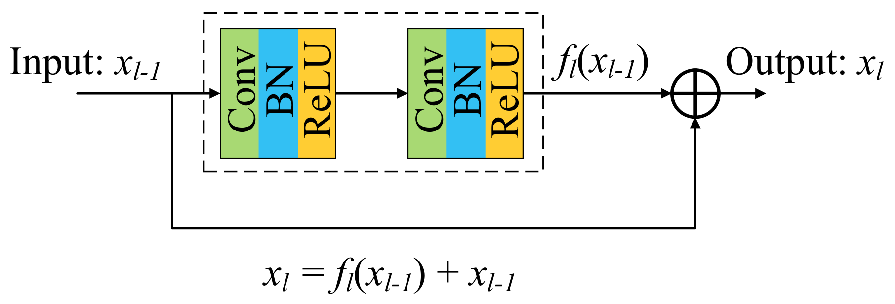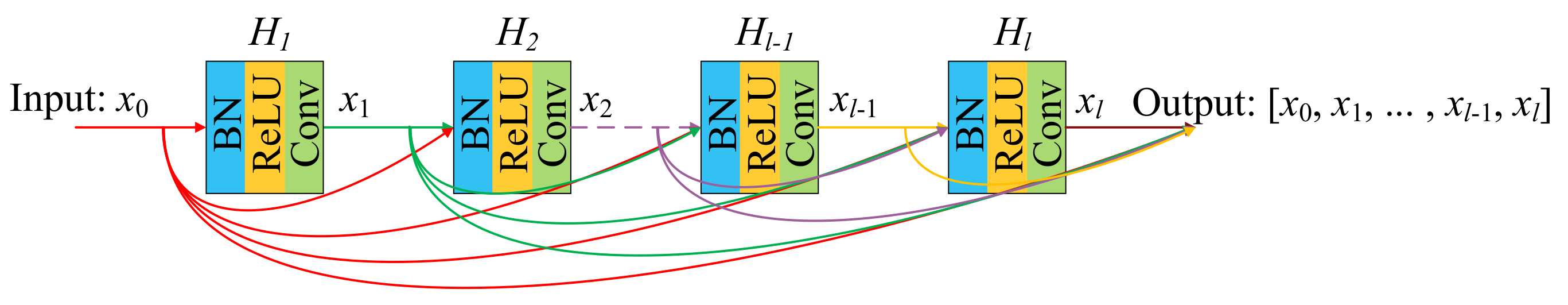In [40], a densely connected CNN (DenseNet) was introduced for HSI classification, which divides the network into dense blocks and creates shortcut connections between layers within each block. This connectivity pattern alleviates the vanishing gradient problem and allows the utilization of various features from different layers for HSI classification. However, only layers within each block are densely connected in the network, which presents local dense connectivity pattern and focuses more on the high level features generated by the last block for HSI classification. These methods have demonstrated that taking advantage of features from different layers in the CNN can achieve good HSI classification performance, but not all of them fully exploit the hierarchical features.

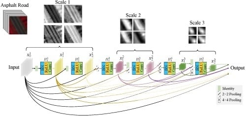
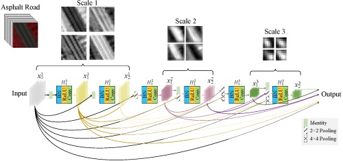
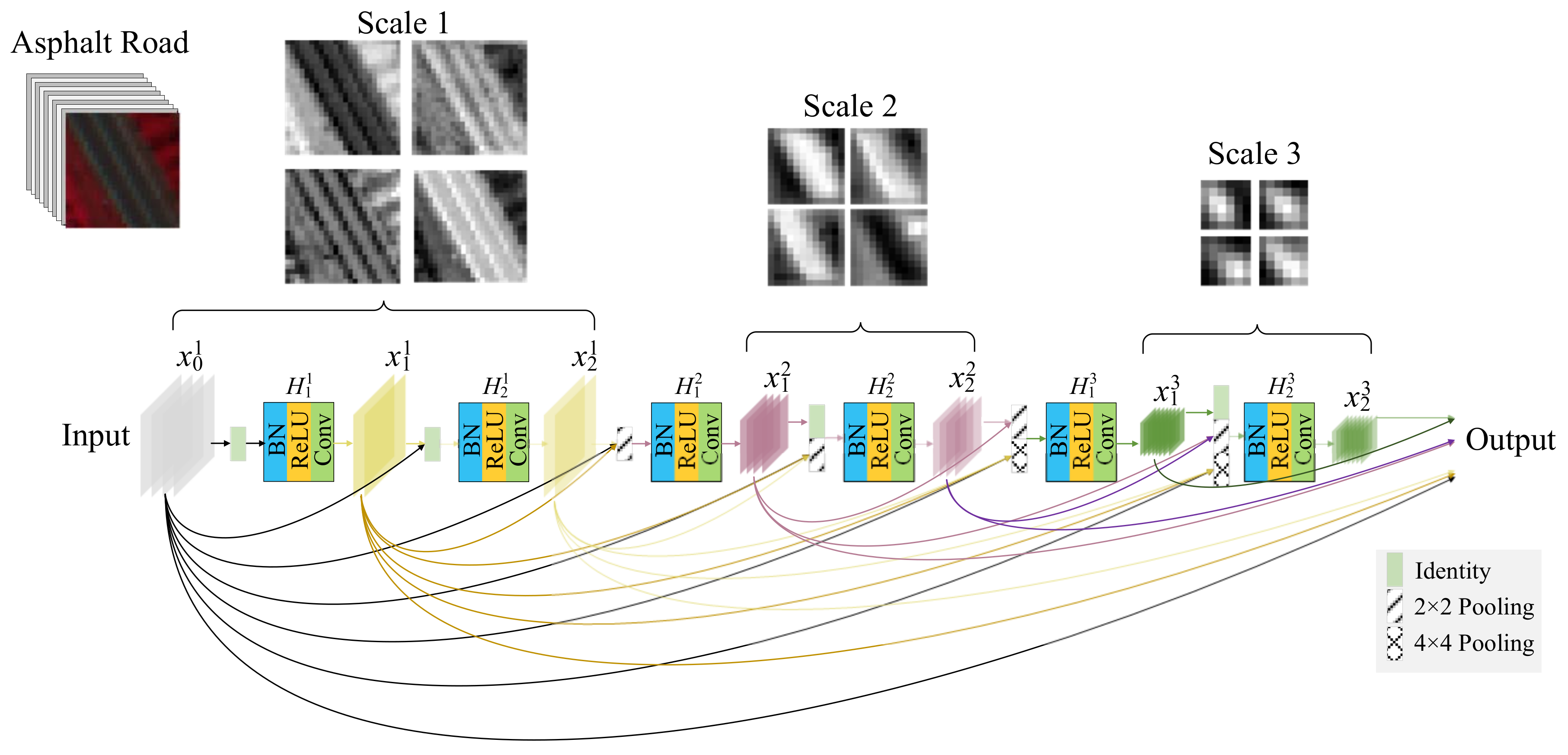
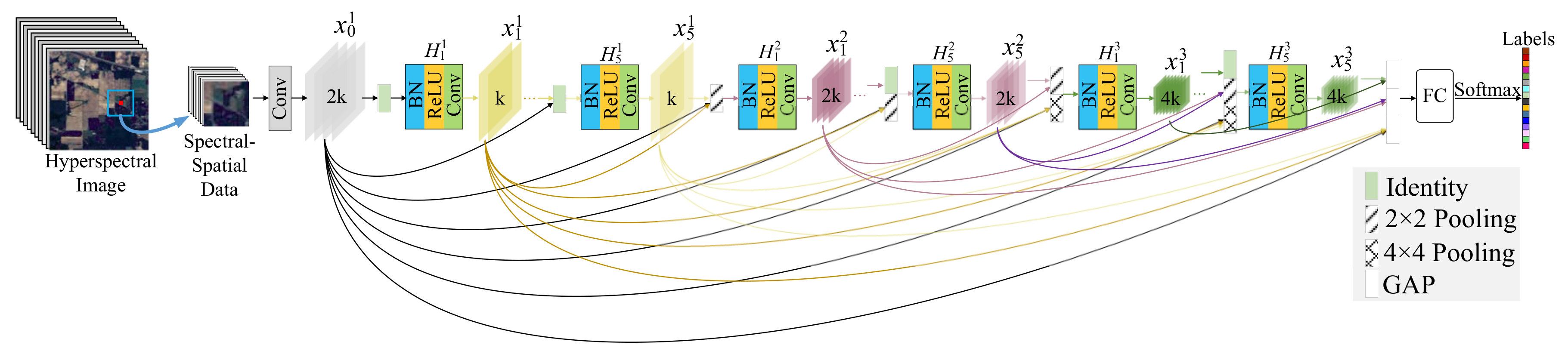
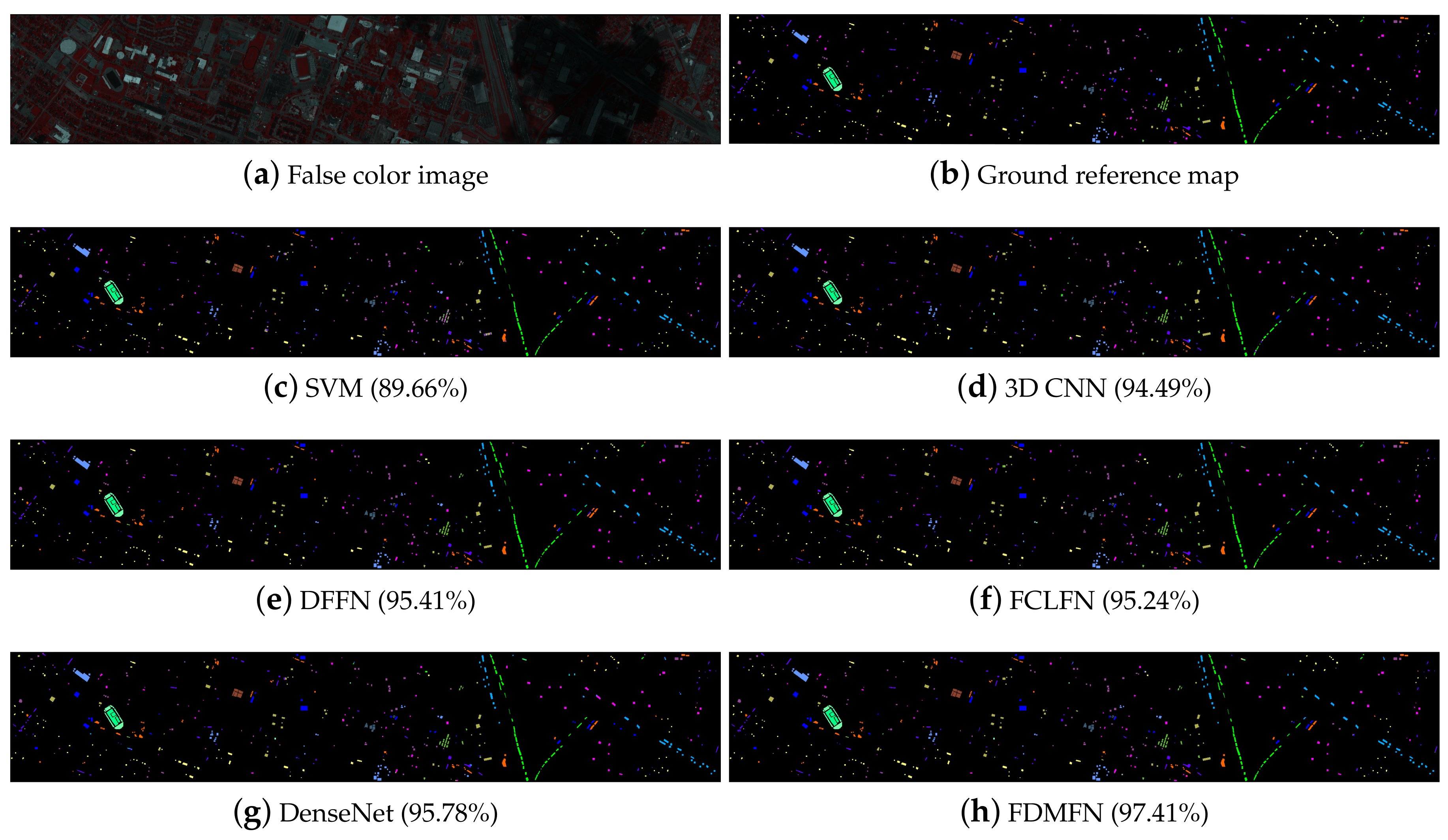
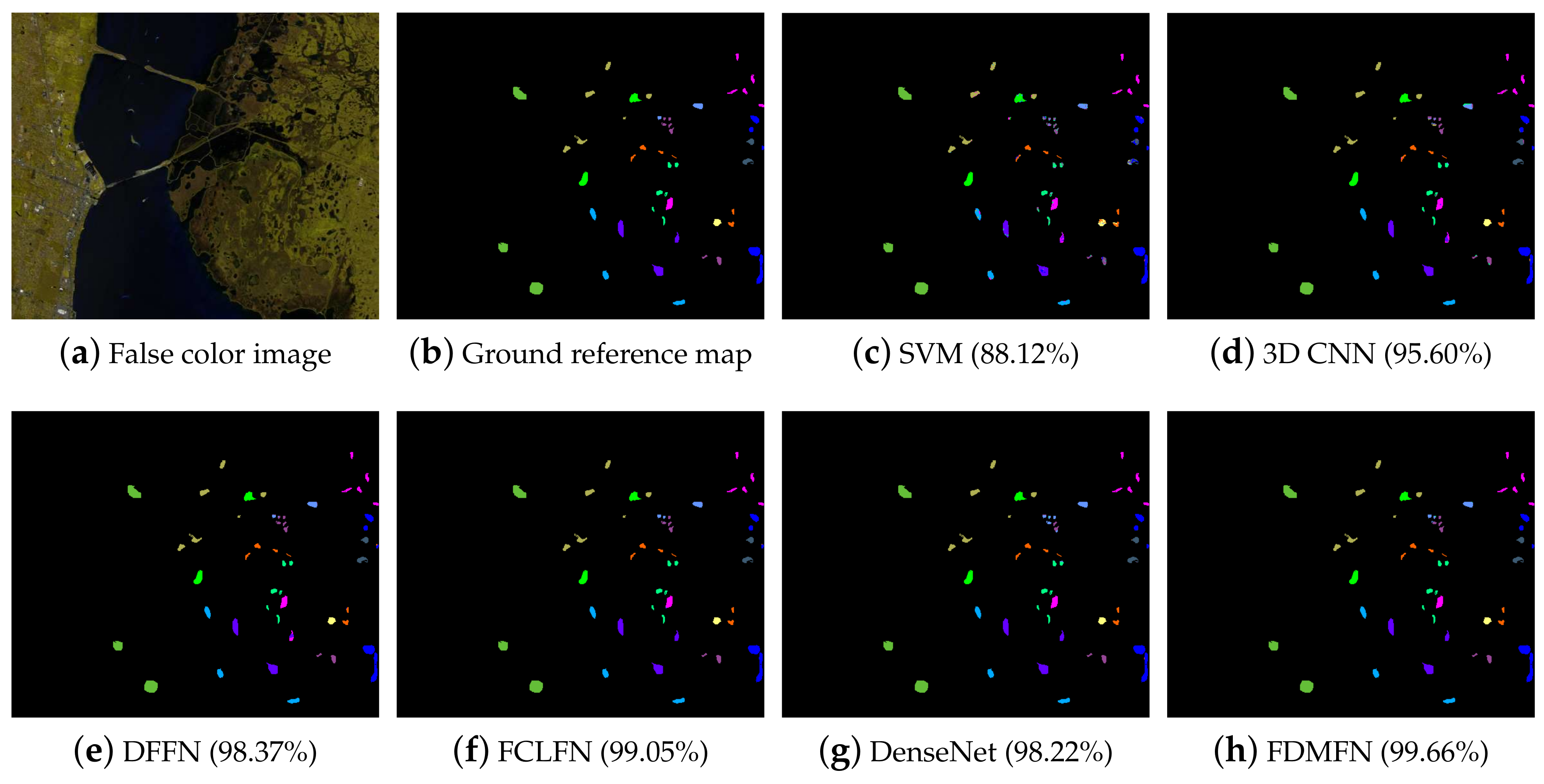
In this paper, inspired by [41], we propose a novel fully dense multiscale fusion network (FDMFN) to achieve full use of the features generated by each convolutional layer for HSI classification. Different from the DenseNet that only introduces dense connections within each block, the proposed method connects any two layers throughout the whole network in a feed-forward fashion, leading to fully dense connectivity. In this way, features from preceding layers are combined as the input of the current layer, and its own output is fed into the subsequent layers, achieving the maximum information flow and feature reuse between layers. In addition, all hierarchical features containing multiscale information are fused to extract more discriminative features for HSI classification. Experimental results conducted on three publicly available hyperspectral scenes demonstrate that the proposed FDMFN can outperform several state-of-the-art approaches, especially under the condition of limited training samples.

In the rest of this paper, Section 2 briefly reviews the CNN based HSI classification procedure. In Section 3, the proposed FDMFN method is described. In Section 4, the experimental results conducted on three real HSIs are reported. In Section 5, we give a discussion on the proposed method and experimental results. Finally, some concluding remarks and possible future works are presented in Section 6.

2. HSI Classification Based on CNN

Deep neural networks can automatically learn hierarchical feature representations from raw HSI data [42,43,44]. Compared with other deep networks, such as SAE [24], DBN [25], and the long short-term memory network (LSTM) [45], CNN can directly take 2D data as input, which provides a natural way to exploit the spatial information of HSIs. Different from natural image classification that uses a whole image input for CNNs, HSI classification, as a pixel level task, generally takes image patches as the input, utilizing the spectral-spatial information contained in each patch to determine the category of its center pixel.

Convolutional (Conv) layers are the fundamental structural elements of CNN models, which use convolution kernels to convolve the input image patches or feature maps to generate various feature maps. Supposing the l^th Conv layer takes $x_{l-1}$ as input, its output $x_l$ can be expressed as:

$$x_l=x_{l-1}*W_l+B_l,$$

(1)

where * represents the convolution operator. $W_l$ and $B_l$ are the weights and biases of the convolution kernels in the l^th Conv layer, respectively.

Behind each Conv layer, a batch normalization (BN) [46] layer is generally attached to accelerate the convergence speed of the CNN model. The procedure of BN can be formulated as:

$$B{N}_{\gamma ,\beta }\left(x_l\right)=\gamma ·\frac{x_l-Mean\left[x_l\right]}{\sqrt{Var\left[x_l\right]+ϵ}}+\beta ,$$

(2)

where the learnable parameter vectors $\gamma$ and $\beta$ are used to scale and shift the normalized feature maps.

To enhance the nonlinearity of the network, the rectified linear unit (ReLU) function [20] is placed behind the BN layer as the activation layer, which is defined as:

$$ReLU\left(x\right)=max(x,0).$$

(3)

In addition, a pooling layer (e.g., average pooling or max pooling) is periodically inserted after several Conv layers to reduce the spatial size of feature maps, which not only reduces the computational cost, but also makes the learned features more invariant with respect to small transformations and distortions of the input data [47].

Finally, the size reduced feature maps are transformed into a feature vector through several fully connected (FC) layers. By feeding the vector into a softmax function, the conditional probability of each class can be obtained, and the predicted class is determined based on the maximum probability.

3. Methodology

3.1. Local Dense Connectivity in DenseNet

It has been demonstrated that introducing shortcut connections in the network alleviates the vanishing gradient problem and enables feature reuse, which can effectively enhance the classification performance [39]. He et al. proposed the residual network (ResNet), which introduces identity shortcut connections to improve the information flow in the network and pushes the depth of the network up to thousands of layers [39]. Deep ResNets can be constructed by stacking residual blocks, in which input features can be passed directly to deeper layers through an additive shortcut connection, as shown in Figure 1.

To further enhance the information flow throughout the network, Huang et al. proposed a different network, called the densely connected convolutional network (DenseNet), in which shortcut connections are employed to concatenate the input features with the output features instead of adding [48]. However, pooling layers, which increase the robustness of the learned features, will change the spatial size of feature maps, resulting in the concatenation operation being unfeasible. To address this problem, Huang et al. divided the network into multiple dense blocks, which do the dense connections in each block and add a pooling layer behind each block, as shown in Figure 2.

Figure 3 shows the architecture of a dense block. Let $x_0$ be the input of the block. For the l^th layer in the block, it receives $x_0$ and features produced by all preceding layers, i.e., $x_1,x_2,\dots ,$ and $x_{l-1}$, as input and its output can be formulated as:

$$x_l=H_l[x_0,x_1,\dots ,x_{l-1}]$$

(4)

where $[·]$ denotes the concatenation operator and $H_l(·)$ is a composite Conv layer with the pre-activation structure of BN-ReLU-Conv [49]. Finally, input features and those generated by each Conv layer are concatenated as the output of the dense block, as shown in Figure 3.

In DenseNet, only layers within each block are densely connected, leading to a local dense connectivity pattern (see Figure 2). In addition, behind the first and second dense blocks, Conv layers are employed to make the extracted features more compact, but the non-dense connections between each block make the network focus more on the high level features (i.e., global coarse and semantic features) extracted by the last dense block for image classification.

3.2. Fully Dense Connectivity

To exploit the hierarchical features from all the Conv layers fully, here, we propose a fully dense connectivity pattern in which shortcut connections are introduced between any two layers in a feed-forward manner, enabling features learned by any layer to be accessed by all subsequent layers. Specifically, the features produced by preceding layers are concatenated as the input of the current layer, and its output features are fed into all the subsequent layers, achieving the maximum information flow. Figure 4 shows the layout of the proposed connectivity pattern schematically. To address the issue that different layers may have different feature map sizes, pooling layers are employed to down-sample feature maps with higher resolutions when they are inputted into lower resolution layers. The average pooling is adopted in this work. Let $x_0^1$ be the initial features extracted from the original HSIs and $x_l^s$ the output of layer l at the s^th scale. Each layer (i.e., $H_l^s$) shown in Figure 4 has the composite structure of BN-ReLU-Conv. For each layer, it receives $x_0^1$ and feature maps produced by all preceding layers.

Table 1. The output $x_l^s$ of layer l at the s^th scale. Herein, $[·]$ represents the concatenation operator. P and $P^2$ refer to the $2\times 2$ and $4\times 4$ pooling layers, respectively.

${\mathit{x}}_{\mathit{l}}^{\mathit{s}}$	$\mathit{l}=1$	$\mathit{l}=2$
$\mathbf{s}=\mathbf{1}$	$H_1^1\left(\left[x_0^1\right]\right)$	$H_2^1\left([x_0^1,x_1^1]\right)$
$\mathbf{s}=\mathbf{2}$	$H_1^2\left(P[x_0^1,x_1^1,x_2^1]\right)$	$H_2^2\left([P[x_0^1,x_1^1,x_2^1],x_1^2]\right)$
$\mathbf{s}=\mathbf{3}$	$H_1^3\left([P^2[x_0^1,x_1^1,x_2^1],P[x_1^2,x_2^2]]\right)$	$H_2^3\left([P^2[x_0^1,x_1^1,x_2^1],P[x_1^2,x_2^2],x_1^3]\right)$

summarizes the output of each layer. For instance, $H_2^1$, Layer 2 at the first scale, receives $x_0^1$ and $x_1^1$ as input, and its output can be computed by $x_2^1=H_2^1\left([x_0^1,x_1^1]\right)$. Note that here, we illustrate the fully dense connectivity with only two Conv layers in each scale, and one can easily deduce situations with more layers by extending Figure 4 and Table 1.

The proposed fully dense connectivity pattern has the following advantages for the classification of HSIs. First, it enhances feature reuse and discriminative feature extraction. As shown in Figure 4, features produced by each Conv layer can be accessed by all subsequent Conv layers, which achieves more comprehensive feature reuse than DenseNet. The reuse of abundant learned features in the subsequent layers is effective for new feature exploration and improves efficiency [48]. In addition, this connectivity pattern further enhances the information flow and alleviates the problem of gradient disappearance. Furthermore, when a classifier is attached behind the output, each intermediate layer will receive an implicit supervision signal through a shorter connection, enforcing them to learn more discriminative and robust features, especially in early layers [50].

Second, the complementary and correlated features from all Conv layers can be exploited for HSI classification. In a CNN model, the receptive field size of Conv layers increases as the number of Conv layers increases [34]. The shallower layers with a narrow receptive field tend to capture local features (e.g., shapes, textures, and lines) of the input objects, whereas the deeper layers with a larger receptive field tend to extract global coarse and semantic features (see Figure 4). Due to the complex spatial environment of HSIs, in which different objects tend to have different scales, only using the global coarse features cannot effectively recognize objects with multiple scales, particularly for those occupying much smaller areas [22]. Through fully dense connectivity, features containing structural information of different scales can be combined for classification, which is beneficial for more accurate recognition of various objects in HSIs.

3.3. Fully Dense Multiscale Fusion Network for HSI Classification

The complete HSI classification framework based on the proposed FDMFN is shown in Figure 5. As an example, consider the Indian Pines (IP) scene: image patches of size $23\times 23\times 200$ from raw image are taken as inputs of FDMFN, fully exploiting the spectral and spatial information. At the beginning, a Conv layer with a $1\times 1$ kernel size is utilized to reduce the dimensionality of input spectral-spatial data and extract features, and therefore, the size of the input is condensed from $23\times 23\times 200$ to $23\times 23\times 2k$, where k is a constant integer referred to as the growth rate, e.g., $k=20$. Next, the obtained features are further processed by a series of $3\times 3$ Conv layers and pooling layers to extract hierarchical feature representations. Note that the number of output features doubles whenever their spatial size shrinks (see Figure 5), because extracting diversified high level features with the increased feature dimension is very effective for classification tasks [51]. After global average pooling (GAP), multiscale hierarchical features from all Conv layers are fused by concatenation to generate more discriminative feature. Finally, the fused feature is fed to a fully connected (FC) layer for classification.

Let $v^m$ be the feature vector learned by the FC layer, where $m=1,2,\dots ,M$ and M is the total number of training samples. For each sample, the probability distribution of each class is obtained by the softmax function, which can be expressed as:

$$p_i^m=\frac{e^{v_i^m}}{{\sum }_{j=1}^T{e}^{v_j^m}},i=1,2,\dots ,T,$$

(5)

where T denotes the total number of classes, $v_i^m$ represents the i^th value of $v^m$, and $p_i^m$ refers to the probability of the m^th training sample belonging to the i^th class. The loss function of FDMFN is defined as:

$$Loss=-\frac{1}{M}\sum _{m=1}^M\sum _{i=1}^T{t}_i^{m}log{p}_i^m,$$

(6)

where $t_i^m$ denotes the ith value of the truth label vector $t^m$. Note that the truth label of each sample is encoded by a vector of length T, in which the position of the correct label is value “1” and all the other positions are value “0”, that is one-hot encoding. The network is trained by minimizing the loss function using the Adam [52] optimization algorithm with 100 epochs. After the optimization is completed, for each test sample, the probability distribution of each class can be obtained by the trained FDMFN, and the predicted label is determined by the maximal probability.

Table 2. FDMFN architecture for the Indian Pines (IP) dataset.

Scale	Conv Layers	Kernel Size	Number of Kernels	Feature Map Size
1	1	$1\times 1$	40	$23\times 23$
1	1–5	$3\times 3$	20	$23\times 23$
$2\times 2$ Average Pooling, Stride 2				$11\times 11$
2	1–5	$3\times 3$	40	$11\times 11$
$2\times 2$ Average Pooling, Stride 2				$5\times 5$
3	1–5	$3\times 3$	80	$5\times 5$
Global Average Pooling				$1\times 1$
16-Dimension Fully Connected Layer, Softmax				-

summarizes the details of the layers of FDMFN for the IP dataset. The stride of convolution is one. Note that for the $3\times 3$ Conv layers, their inputs are zero padded with one pixel on each side to keep the spatial size of feature maps fixed during convolution.

4. Experiments

4.1. Description of Datasets

Three publicly available hyperspectral datasets were utilized to verify the effectiveness of our FDMFN method, i.e., Indian Pines (IP), University of Houston (UH), and Kennedy Space Center (KSC) datasets [53,54].

The IP dataset was gathered in 1992 by the Airborne Visible/Infrared Imaging Spectrometer (AVIRIS) instrument [55] from Northwest Indiana. This dataset mainly covers a mixed agricultural/forest area, consisting of 145 × 145 pixels and 224 spectral bands in the spectral range from 400 to 2500 nm. The geometric resolution is 20 m by pixel, and the ground reference map has 16 classes. After discarding four null bands and another 20 water absorption bands, 200 channels were utilized for the experiments.

The UH dataset was gathered in 2012 by the Compact Airborne Spectrographic Imager (CASI) sensor [56] over the campus of the University of Houston and its neighboring region. It was first presented in the 2013 Geoscience and Remote Sensing Society (GRSS) Data Fusion Contest [57]. This scene is composed of 349 × 1905 pixels, and its ground reference map contains 15 classes. The geometric resolution is 2.5 m by pixel. It has 144 spectral bands in the spectral range from 380 to 1050 nm.

The KSC dataset was acquired in 1996 by the AVIRIS instrument [55] in Florida with a geometric resolution of 18 m by pixel. This scene consists of 512 × 614 pixels and mainly includes 13 classes. After discarding noisy bands, the considered scene had 176 spectral bands for the classification.

In our experiments, the labeled samples of each dataset were divided into training, validation, and testing sets, and the split ratio was 5%:5%:90%.

Table 3. Number of samples of the IP dataset.

Class	Color	Land-Cover Type	Training	Validation	Testing
1		Alfalfa	3	3	40
2		Corn-notill	72	72	1284
3		Corn-mintill	42	42	746
4		Corn	12	12	213
5		Grass-pasture	25	25	433
6		Grass-trees	37	37	656
7		Grass-pasture-mowed	2	2	24
8		Hay-windrowed	24	24	430
9		Oats	1	1	18
10		Soybean-notill	49	49	874
11		Soybean-mintill	123	123	2209
12		Soybean-clean	30	30	533
13		Wheat	11	11	183
14		Woods	64	64	1137
15		Buildings-Grass-Trees	20	20	346
16		Stone-Steel-Towers	5	5	83
		Total Number	520	520	9209

,

Table 4. Number of samples of the University of Houston (UH) dataset.

Class	Color	Land-Cover Type	Training	Validation	Testing
1		Healthy grass	63	63	1125
2		Stressed grass	63	63	1128
3		Synthetic grass	35	35	627
4		Trees	63	63	1118
5		Soil	63	63	1116
6		Water	17	17	291
7		Residential	64	64	1140
8		Commercial	63	63	1118
9		Road	63	63	1126
10		Highway	62	62	1103
11		Railway	62	62	1111
12		Parking Lot1	62	62	1109
13		Parking Lot2	24	24	421
14		Tennis court	22	22	384
15		Running track	33	33	594
		Total Number	759	759	13,511

and

Table 5. Number of samples of the Kennedy Space Center (KSC) dataset.

Class	Color	Land-Cover Type	Training	Validation	Testing
1		Scrub	39	39	683
2		Willow swamp	13	13	217
3		CP hammock	13	13	230
4		Slash pine	13	13	226
5		Oak/Broadleaf	9	9	143
6		Hardwood	12	12	205
7		Swamp	6	6	93
8		Graminoid marsh	22	22	387
9		Spartina marsh	26	26	468
10		Cattail marsh	21	21	362
11		Salt marsh	21	21	377
12		Mud flats	26	26	451
13		Water	47	47	833
		Total Number	268	268	4675

summarize the number of samples of the three datasets. Note that the network parameters were only tuned using the training set. During the training phase, the interim trained model that achieved the highest classification performance on the validation set was saved. Finally, the testing set was used to evaluate the preserved model’s classification performance. Three widely used quantitative metrics, overall accuracy (OA), average accuracy (AA), and the Kappa coefficient [58], were adopted to assess the classification performance. To avoid biased estimation, all experiments were repeated five times with randomly selected training samples, and the average values were reported for all the performance metrics.

4.2. Experimental Setup

We trained the proposed network for 100 epochs using the Adam [52] optimizer with batch size of 100 as done in [40]. The network parameters were initialized by using the He initialization method [59]. We used an L2 weight decay penalty of 0.0001 and a cosine shape learning rate, which began from 0.001 and gradually decreased to zero [60]. The proposed network was implemented by using the Pytorch framework [61]. All the experiments were conducted on a PC with a single NVIDIA GeForce RTX 2080 GPU and an AMD Ryzen 7 2700X CPU.

4.3. Analysis of Parameters

In the proposed FDMFN method, except the weights and biases of the network, which could be tuned automatically during the training phase, the number of Conv layers, the growth rate k, and the size of input image patches were also important to the final classification performance.

Figure 6a shows the impact of the number of Conv layers on the average accuracy (AA) of the proposed FDMFN. The number of Conv layers determines the network depth, which is an important parameter that can affect the classification performance. Although a deeper network can learn more abstract features for classification, it will increase the possibility of overfitting. From Figure 6a, one can see that the best AA value was achieved when the number of Conv layers was 16 for the IP dataset. For the UH and KSC datasets, the AA values could reach the highest when the number of Conv layers was 13. Therefore, in the following experiments, the number of Conv layers was set to 16, 13, and 13 for the IP, UH, and KSC datasets, respectively.

Figure 6b illustrates the influence of the growth rate k on the AA of the proposed method. The parameter k also determines the representation capacity of the proposed FDMFN. We assessed different k values from 8 to 24 with a step of 4 for each dataset. As shown in Figure 6b, when k was 20, the model obtained the best performance on the IP dataset. For the UH and KSC datasets, when k was 12, the models achieved the highest classification accuracy. Therefore, k was set to 20, 12, and 12 for the IP, UH, and KSC datasets, respectively.

Figure 6c shows the tendencies of AA of the proposed FDMFN over different sizes of input image patches. As can be seen, with the increase of the patch size, the AA values tended to increase first and then decrease on the three datasets. Generally speaking, a larger size of image patch would bring more spatial information, which would help to increase the classification accuracy. However, a large image patch may contain pixels belonging to multiple classes, misleading the classification of the target pixel. From Figure 6c, one can see that when the patch size was $23\times 23$, the proposed FDMFN could produce the best classification results for all three datasets. Therefore, we chose $23\times 23$ as the default size of input image patches.

4.4. Compared Methods

We compared our FDMFN method with several well known classification approaches, including SVM with radial basis function (RBF) kernel [5], 3D CNN [32], the deep feature fusion network (DFFN) [37], the fully convolutional layer fusion network (FCLFN) [38], and DenseNet [40].

Specifically, SVM only exploits the spectral information embedded in HSIs for classification. The remaining are spectral-spatial based classification methods. 3D CNN directly extracts spectral-spatial features from original HSIs using 3D convolutional kernels. DFFN fuses spectral-spatial features generated at different stages in a deep residual network for the classification of HSIs. FCLFN fuses spectral-spatial features produced by all Conv layers for HSI classification. For DenseNet, due to the local dense connectivity pattern, only spectral-spatial features from layers in the last block were fully combined for HSI classification. In addition, for SVM, the penalty parameter C and the RBF kernel parameter $\gamma$ were determined through five-fold cross-validation ($C=2^{-8},2^{-7},\dots ,2^8,\gamma =2^{-8},2^{-7},\dots ,2^8$). For other methods, we used the default parameter setting in the corresponding references [32,37,38,40]. Take the Indian Pines dataset as an example: for the DFFN, FCLFN, and DenseNet methods, the default size of input image patches was $25\times 25$, $23\times 23$, and $11\times 11$, respectively.

4.5. Classification Results

Figure 7 shows the classification maps obtained by various approaches on the IP dataset (all the classification maps were the result of the first experiment of the five experiments). One can see that the SVM classifier generated rather poor estimations in its classification map (see Figure 7c), as it only exploited the spectral information of HSI. In contrast, by utilizing spatial and spectral information, the other methods showed better visual performances in their classification maps (see Figure 7d–h).

Table 6. Classification accuracies (in %) of different methods for the IP dataset using 5% of labeled samples for training. The best results are highlighted in bold font.

Class	Color	SVM [5]	3D CNN [32]	DFFN [37]	FCLFN [38]	DenseNet [40]	FDMFN
1		38.14	86.50	61.50	54.00	79.50	97.00
2		72.48	94.67	94.47	96.15	97.38	97.21
3		61.22	90.75	93.62	95.71	96.22	96.81
4		45.51	92.39	92.49	95.49	98.40	98.40
5		84.72	91.09	82.96	92.79	92.75	94.23
6		94.08	97.96	94.66	97.01	98.84	97.10
7		59.23	81.67	45.00	20.83	82.50	91.67
8		95.73	99.21	99.77	99.86	99.95	99.91
9		12.63	77.78	3.33	0.00	63.33	81.11
10		64.27	88.49	92.59	92.61	95.40	95.65
11		74.41	93.55	95.38	97.02	94.73	97.22
12		56.09	89.68	87.05	90.43	90.47	92.05
13		96.08	96.17	93.44	94.64	99.02	98.47
14		93.34	97.55	96.55	98.17	99.05	98.14
15		46.39	87.92	92.02	96.71	89.13	95.90
16		82.73	91.08	48.67	57.83	97.59	90.12
OA		74.73	93.43	92.97	95.05	95.84	96.72
AA		67.32	91.03	79.59	79.95	92.14	95.06
Kappa		71.13	92.51	91.98	94.35	95.26	96.26

presents the quantitative results of different methods. One can see that the proposed FDMFN outperformed the contrastive approaches in terms of three overall metrics (i.e., OA, AA, and Kappa), demonstrating the effectiveness of our method. Note that the class distribution of this dataset was quite unbalanced. The largest class, soybean-mintill (Category 11), contained 2455 samples, while the smallest class, oats (Category 9), had only 20 samples. When facing a dataset with an uneven class distribution, the minority classes may be heavily underrepresented, leading to poor classification performance. From Table 6, one can see that SVM, DFFN, FCLFN, and DenseNet achieved rather poor results on the oats class (Category 9). However, the proposed FDMFN avoided this problem and achieved the highest classification accuracy on the oats class, again verifying the effectiveness of our method.

Table 7. Classification accuracies (in %) of different methods for the UH dataset using 5% of labeled samples for training. The best results are highlighted in bold font.

Class	Color	SVM [5]	3D CNN [32]	DFFN [37]	FCLFN [38]	DenseNet [40]	FDMFN
1		96.13	98.12	97.26	91.95	98.68	97.24
2		95.75	98.00	96.21	97.22	98.69	98.39
3		99.37	98.76	99.01	98.66	99.55	98.69
4		96.09	95.33	91.11	90.21	92.83	96.51
5		98.34	99.71	99.39	99.80	99.98	100
6		89.87	92.16	89.07	87.49	87.15	90.72
7		89.55	92.93	94.58	92.89	93.49	95.77
8		84.35	83.38	88.89	90.21	89.02	93.70
9		79.43	89.22	94.60	93.84	90.73	96.38
10		91.54	96.08	98.98	99.96	96.46	100
11		85.88	92.91	97.01	97.32	97.98	98.18
12		83.77	94.30	94.52	97.44	97.94	98.30
13		43.46	90.40	91.73	92.21	91.83	94.01
14		97.64	99.90	100	100	100	100
15		98.92	99.80	97.41	97.68	99.97	99.56
OA		89.66	94.49	95.41	95.24	95.78	97.41
AA		88.67	94.73	95.32	95.13	95.62	97.16
Kappa		88.82	94.04	95.04	94.85	95.44	97.20

and

Table 8. Classification accuracies (in %) of different methods for the KSC dataset using 5% of labeled samples for training. The best results are highlighted in bold font.

Class	Color	SVM [5]	3D CNN [32]	DFFN [37]	FCLFN [38]	DenseNet [40]	FDMFN
1		92.27	98.68	98.92	98.89	99.88	100
2		84.17	86.54	92.81	90.88	95.48	98.99
3		80.08	94.17	99.04	99.83	96.35	99.83
4		61.51	78.41	95.93	95.93	84.78	95.84
5		50.66	66.71	91.05	96.50	92.87	98.18
6		53.64	92.00	97.07	99.32	96.59	99.71
7		75.56	96.77	100	100	97.42	100
8		89.34	97.67	98.14	99.84	99.74	100
9		94.82	98.42	97.78	100	100	100
10		93.00	99.78	99.56	99.89	99.61	100
11		94.42	99.95	100	100	99.79	99.84
12		92.37	95.34	99.20	100	98.45	99.96
13		100	100	100	100	100	100
OA		88.12	95.60	98.37	99.05	98.22	99.66
AA		81.68	92.65	97.65	98.54	97.00	99.41
Kappa		86.77	95.10	98.19	98.94	98.02	99.62

report the quantitative classification results (obtained by averaging of five runs) on the UH and KSC datasets, respectively. Figure 8 and Figure 9 separately show the corresponding classification maps. Compared with DenseNet, FDMFN improved the OA from 95.78% to 97.41% for the UH dataset. Moreover, FDMFN achieved significant performance gains over DenseNet with 2.41% in terms of AA for the KSC dataset. Overall, FDMFN outperformed all other compared methods in terms of the three overall metrics on the two datasets, which validated the effectiveness of our method.

To demonstrate whether the accuracy improvement of the proposed FDMFN over the compared methods was statistically significant, we performed the standardized McNemar’s test [62], which is defined as:

$$Z={\displaystyle \frac{f_{12}-f_{21}}{\sqrt{f_{12}-f_{21}}}},$$

(7)

where $f_{ij}$ denotes the number of samples that are correctly classified by classifier i and incorrectly classified by classifier j. When Z is larger than 2.58, it means that the performance improvement of Classifier 1 over Classifier 2 is statistically significant at the 99% confidence level. As shown in

Table 9. Statistical significance of the improvement of FDMFN over other methods.

IP	UH	KSC
Z/Significant?	Z/Significant?	Z/Significant?
FDMFN vs. SVM
44.98/yes	32.35/yes	23.14/yes
FDMFN vs. 3D CNN
17.20/yes	19.61/yes	13.70/yes
FDMFN vs. DFFN
18.03/yes	16.41/yes	7.52/yes
FDMFN vs. FCLFN
12.24/yes	16.88/yes	4.85/yes
FDMFN vs. DenseNet
8.63/yes	13.98/yes	8.14/yes

, all the Z values were much higher than 2.58, which confirmed that our FDMFN method significantly outperformed the contrastive approaches.

Finally, the computing times of the proposed FDMFN and other deep neural networks on the three datasets are reported in

Table 10. Training and test times (in seconds) on the three datasets using different deep neural networks.

		IP	UH	KSC
3D CNN	Training	33.88	36.92	15.35
	Test	1.88	2.11	0.87
DFFN	Training	14.92	20.79	7.92
	Test	0.61	0.92	0.32
FCLFN	Training	13.28	18.07	7.14
	Test	0.59	0.90	0.30
DenseNet	Training	33.13	42.47	16.40
	Test	1.56	1.97	0.73
FDMFN	Training	55.19	50.31	23.75
	Test	4.00	3.86	1.85

. One can see that FCLFN consumed the lowest time, while the proposed FDMFN was the most time consuming on the three datasets, because of there being more parameters in FDMFN than other compared models on the IP dataset (see

Table 11. Numbers of trainable parameters in different deep neural networks.

	3D CNN	DFFN	FCLFN	DenseNet	FDMFN
IP	0.10M	0.40M	0.17M	1.67M	2.30M
UH	0.07M	0.40M	0.17M	1.66M	0.54M
KSC	0.08M	0.40M	0.16M	1.66M	0.54M

). For the UH and KSC datasets, although FDMFN had fewer parameters than DenseNet, it took a larger size of image patch as input ($23\times 23$ for FDMFN and $11\times 11$ for DenseNet [40]) and thus also spent more time than DenseNet. Although time consuming, FDMFN could achieve better classification performance in comparison with other deep networks.

4.6. Effect of Different Ratios of Training Samples

In this section, the effectiveness and robustness of the proposed method are investigated when different ratios of training samples were considered. For each dataset, the ratio of training samples ranged from 2% to 10% with an interval of 2%. The OA values obtained by different methods on the three datasets are illustrated in Figure 10. It can be observed that FDMFN provided better classification accuracies in comparison with other methods under all different ratios of training samples. Furthermore, with less training samples (e.g., using only 2% of training samples), the proposed FDMFN had significant advantage over other compared approaches on the IP and KSC datasets.

4.7. Input Patch Size Analysis

In general, larger input HSI patches with more spatial information tend to have an advantage over the ones with less spatial information. However, larger input patches may contain pixels from multiple classes, which confuse the recognition of the target pixel. In addition, it reduces the inter-sample diversity and increases the possibility of overfitting. In this experiment, we further compared the proposed method with other deep neural networks when they shared the same size of input HSI patches. The experiment was implemented on the KSC dataset, and the spatial size varied in the set {$11\times 11$, $15\times 15$, $19\times 19$, $23\times 23$, and $27\times 27$}. For the small spatial size (e.g., $11\times 11$), we removed the pooling layers due to the rapid down-sampling of the input image patch. The overall accuracies obtained from different methods are shown in

Table 12. Overall accuracy (in %) obtained by different approaches on the KSC dataset when considering different spatial sizes of input patches. The best results are highlighted in bold font.

Spatial Size	3D CNN	DFFN	FCLFN	DenseNet	FDMFN
$11\times 11$	95.91	81.83	94.98	97.60	98.47
$15\times 15$	97.01	88.56	97.97	99.01	99.17
$19\times 19$	97.67	94.22	98.24	99.26	99.44
$23\times 23$	98.08	97.82	98.74	99.35	99.66
$27\times 27$	98.08	98.18	98.98	99.28	99.43

. As can be seen, the proposed FDMFN outperformed other methods regardless of the spatial sizes of the input HSI patches, which demonstrated the effectiveness of the proposed FDMFN method. In addition, all the overall accuracies obtained by the proposed method with different patch sizes were higher than 98%, which suggests that our FDMFN method is robust to the spatial size of input patches.

4.8. Comparison with Other State-of-the-Art Approaches

In this section, we further compared the proposed FDMFN method with another three state-of-the-art deep learning based HSI classification approaches: the dilated convolution based CNN model (Dilated-CNN) [28], the 2D spectrum based CNN model [29], and the artificial neuron network with center-loss and adaptive spatial-spectral center classifier (ANNC-ASSCC) [30].

Specifically, we first compared the proposed method with the Dilated-CNN on the IP and Salinas datasets. The detailed information of the Salinas dataset can be also found in [53]. Following Dilated-CNN [28], for each dataset, 60% of the labeled samples per class were randomly selected for training. Next, the proposed FDMFN was compared with the 2D spectrum based CNN model [29] on the IP, KSC, and Salinas datasets. For a fair comparison, we utilized the same number of samples, as in [29], for model training. Finally, the proposed method was compared with the ANNC-ASSCC method [30] on the Salinas dataset. Following [30], we randomly chose 200 labeled samples from each class for training.

The corresponding classification results are shown in

Table 13. Comparison between the proposed FDMFN and the Dilated-CNN [28] method on the IP and Salinas datasets. Note that the best results reported in [28] were used for comparison here. In addition, the best results are highlighted in bold font.

	IP		Salinas
	Dilated-CNN [28]	FDMFN	Dilated-CNN [28]	FDMFN
OA (%)	99.81	99.95	99.99	100
AA (%)	99.83	99.93	99.98	100
Kappa (%)	98.68	99.95	99.99	100

,

Table 14. Comparison between the proposed FDMFN and the 2D spectrum based CNN model [29] on the IP, KSC, and Salinas datasets. Note that the best results reported in [29] were used for comparison here. In addition, the best results are highlighted in bold font.

	IP		KSC		Salinas
	[29]	FDMFN	[29]	FDMFN	[29]	FDMFN
OA(%)	98.26	99.98	96.22	99.83	97.28	99.78
Kappa	0.978	0.9998	0.956	0.9981	0.962	0.9974

and

Table 15. Comparison between the proposed FDMFN and the artificial neuron network with center-loss and adaptive spatial-spectral center classifier (ANNC-ASSCC) [30] on the Salinas dataset. Note that the best results reported in [30] were used for comparison here. In addition, the best results are highlighted in bold font.

	ANNC-ASSCC [30]	FDMFN
OA(%)	96.98	99.94
AA(%)	98.81	99.95
Kappa(%)	96.62	99.93

. As can be observed, the proposed method achieved improved performance in comparison with the other three deep learning models. By making full use of the hierarchical features, our method could exploit multiscale information for the classification of HSIs. In addition, the comprehensive feature reuse in the proposed network also facilitated discriminative feature learning. The results shown in Table 13, Table 14 and Table 15 further demonstrate the superiority of our FDMFN model for HSI classification.

5. Discussion

There are mainly two reasons why FDMFN achieved a superior classification performance. First, the proposed method achieved comprehensive reuse of abundant information from different layers and provided additional supervision for each intermediate layer, enforcing discriminant feature learning. Second, the multiscale hierarchical features learned by all Conv layers were combined for HSI classification, which allowed finer recognition of various objects and hence enhancing the classification performance.

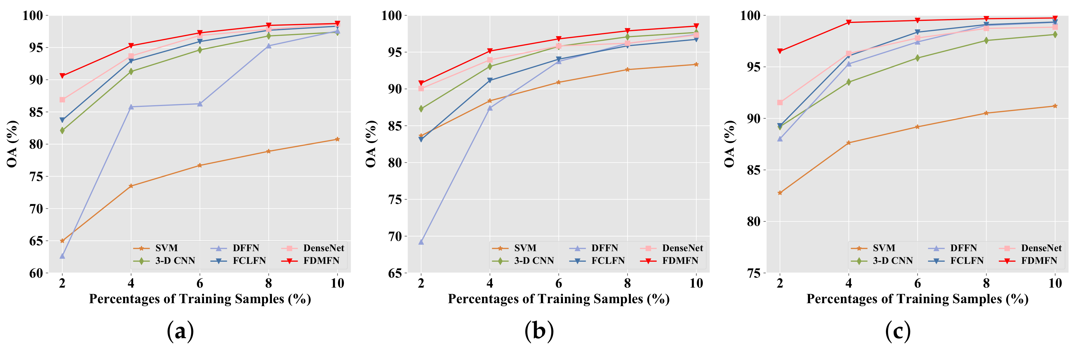
From the comparison of the execution time of different deep neural networks, we can find that the proposed model was not computationally efficient. However, our method could achieve better classification performance in comparison with other methods on the three real hyperspectral datasets. Furthermore, when limited training samples were utilized, the proposed method significantly outperformed other approaches on the IP and KSC datasets, further demonstrating its effectiveness for HSI classification. In our future work, to reduce the computational load, a memory efficient implementation of the proposed network will be investigated.

6. Conclusions

In this work, we proposed a novel FDMFN to fully exploit the hierarchical features from all Conv layers for spectral-spatial HSI classification. The proposed FDMFN was characterized by introducing shortcut connections between any two layers in the network. Through fully dense connectivity, the spectral-spatial features learned by each layer could be accessed by all subsequent layers, achieving comprehensive feature reuse. In addition, the proposed method enforced discriminative feature learning by providing additional supervision. Furthermore, multiscale features extracted by all Conv layers were fused to extract more discriminative features for HSI classification. Experimental results on three widely used hyperspectral scenes demonstrated that the proposed FDMFN outperformed other state-of-the-art methods.

Note that although the combination of all hierarchical features provided a good classification performance, the contribution from features with different scales varied for different objects. In our future work, attention mechanisms [63] will be considered to adaptively emphasize representative features and suppress less useful ones for each sample, to enhance the classification performance further.

References

1. Olmanson, L.G.; Brezonik, P.L.; Bauer, M.E. Airborne hyperspectral remote sensing to assess spatial distribution of water quality characteristics in large rivers: The Mississippi River and its tributaries in Minnesota. Remote Sens. Environ. 2013, 130, 254–265. [Google Scholar] [CrossRef]
2. Zhang, L.; Zhang, L.; Du, B. Deep learning for remote sensing data: A technical tutorial on the state of the art. IEEE Geosci. Remote Sens. Mag. 2016, 4, 22–40. [Google Scholar] [CrossRef]
3. Zhang, X.; Sun, Y.; Shang, K.; Zhang, L.; Wang, S. Crop classification based on feature band set construction and object-oriented approach using hyperspectral images. IEEE J. Sel. Top. Appl. Earth Obs. Remote Sens. 2016, 9, 4117–4128. [Google Scholar] [CrossRef]
4. Li, S.; Song, W.; Fang, L.; Chen, Y.; Ghamisi, P.; Benediktsson, J.A. Deep learning for hyperspectral image classification: An overview. IEEE Trans. Geosci. Remote Sens. 2019, 57, 6690–6709. [Google Scholar] [CrossRef]
5. Melgani, F.; Bruzzone, L. Classification of hyperspectral remote sensing images with support vector machines. IEEE Trans. Geosci. Remote Sens. 2004, 42, 1778–1790. [Google Scholar] [CrossRef]
6. Zhang, L.; Zhang, L.; Tao, D.; Huang, X. On combining multiple features for hyperspectral remote sensing image classification. IEEE Trans. Geosci. Remote Sens. 2012, 50, 879–893. [Google Scholar] [CrossRef]
7. Ham, J.; Chen, Y.; Crawford, M.M.; Ghosh, J. Investigation of the random forest framework for classification of hyperspectral data. IEEE Trans. Geosci. Remote Sens. 2005, 43, 492–501. [Google Scholar] [CrossRef]
8. Li, J.; Bioucas-Dias, J.M.; Plaza, A. Semisupervised hyperspectral image segmentation using multinomial logistic regression with active learning. IEEE Trans. Geosci. Remote Sens. 2010, 48, 4085–4098. [Google Scholar] [CrossRef]
9. Fauvel, M.; Tarabalka, Y.; Benediktsson, J.A.; Chanussot, J.; Tilton, J.C. Advances in spectral-spatial classification of hyperspectral images. Proc. IEEE 2013, 101, 652–675. [Google Scholar] [CrossRef]
10. He, L.; Li, J.; Liu, C.; Li, S. Recent advances on spectral-spatial hyperspectral image classification: An overview and new guidelines. IEEE Trans. Geosci. Remote Sens. 2018, 56, 1579–1597. [Google Scholar] [CrossRef]
11. Benediktsson, J.A.; Palmason, J.A.; Sveinsson, J.R. Classification of hyperspectral data from urban areas based on extended morphological profiles. IEEE Trans. Geosci. Remote Sens. 2005, 43, 480–491. [Google Scholar] [CrossRef]
12. Kang, X.; Li, S.; Benediktsson, J.A. Spectral-spatial hyperspectral image classification with edge-preserving filtering. IEEE Trans. Geosci. Remote Sens. 2014, 52, 2666–2677. [Google Scholar] [CrossRef]
13. Camps-Valls, G.; Bruzzone, L. Kernel-based methods for hyperspectral image classification. IEEE Trans. Geosci. Remote Sens. 2005, 43, 1351–1362. [Google Scholar] [CrossRef]
14. Peng, J.; Zhou, Y.; Chen, C.L.P. Region-kernel-based support vector machines for hyperspectral image classification. IEEE Trans. Geosci. Remote Sens. 2015, 53, 4810–4824. [Google Scholar] [CrossRef]
15. Chen, Y.; Nasrabadi, N.M.; Tran, T.D. Hyperspectral image classification using dictionary-based sparse representation. IEEE Trans. Geosci. Remote Sens. 2011, 49, 3973–3985. [Google Scholar] [CrossRef]
16. Fang, L.; Li, S.; Kang, X.; Benediktsson, J.A. Spectral-spatial hyperspectral image classification via multiscale adaptive sparse representation. IEEE Trans. Geosci. Remote Sens. 2014, 52, 7738–7749. [Google Scholar] [CrossRef]
17. Fang, L.; Li, S.; Duan, W.; Ren, J.; Benediktsson, J.A. Classification of hyperspectral images by exploiting spectral-spatial information of superpixel via multiple kernels. IEEE Trans. Geosci. Remote Sens. 2015, 53, 6663–6674. [Google Scholar] [CrossRef]
18. Mou, L.; Zhu, X.X. Unsupervised spectral-spatial feature learning via deep residual Conv-Deconv network for hyperspectral image classification. IEEE Trans. Geosci. Remote Sens. 2018, 56, 391–406. [Google Scholar] [CrossRef]
19. Szegedy, C.; Liu, W.; Jia, Y.; Sermanet, P.; Reed, S.; Anguelov, D.; Erhan, D.; Vanhoucke, V.; Rabinovich, A. Going deeper with convolutions. In Proceedings of the IEEE Conference on Computer Vision and Pattern Recognition (CVPR), Boston, MA, USA, 7–12 June 2015; pp. 1–9. [Google Scholar]
20. Krizhevsky, A.; Sutskever, I.; Hinton, G.E. Imagenet classification with deep convolutional neural networks. In Proceedings of the International Conference on Neural Information Processing Systems (NIPS), Lake Tahoe, NV, USA, 3–6 December 2012; pp. 1097–1105. [Google Scholar]
21. Li, W.; Wu, G.; Zhang, F.; Du, Q. Hyperspectral image classification using deep pixel-pair features. IEEE Trans. Geosci. Remote Sens. 2017, 55, 844–853. [Google Scholar] [CrossRef]
22. Jiao, L.; Liang, M.; Chen, H.; Yang, S.; Liu, H.; Cao, X. Deep fully convolutional network-based spatial distribution prediction for hyperspectral image classification. IEEE Trans. Geosci. Remote Sens. 2017, 55, 5585–5599. [Google Scholar] [CrossRef]
23. Meng, Z.; Li, L.; Tang, X.; Feng, Z.; Jiao, L.; Liang, M. Multipath residual network for spectral-spatial hyperspectral image classification. Remote Sens. 2019, 11, 1896. [Google Scholar] [CrossRef]
24. Chen, Y.; Lin, Z.; Zhao, X.; Wang, G.; Gu, Y. Deep learning-based classification of hyperspectral data. IEEE J. Sel. Top. Appl. Earth Obs. Remote Sens. 2014, 7, 2094–2107. [Google Scholar] [CrossRef]
25. Chen, Y.; Zhao, X.; Jia, X. Spectral-spatial classification of hyperspectral data based on deep belief network. IEEE J. Sel. Top. Appl. Earth Obs. Remote Sens. 2015, 8, 2381–2392. [Google Scholar] [CrossRef]
26. Zhang, H.; Li, Y.; Zhang, Y.; Shen, Q. Spectral-spatial classification of hyperspectral imagery using a dual-channel convolutional neural network. Remote Sens. Lett. 2017, 8, 438–447. [Google Scholar] [CrossRef]
27. Zhao, W.; Du, S. Spectral-spatial feature extraction for hyperspectral image classification: A dimension reduction and deep learning approach. IEEE Trans. Geosci. Remote Sens. 2016, 54, 4544–4554. [Google Scholar] [CrossRef]
28. Devaram, R.R.; Allegra, D.; Gallo, G.; Stanco, F. Hyperspectral image classification via convolutional neural network based on dilation layers. In Proceedings of the International Conference on Image Analysis and Processing (ICIAP), Trento, Italy, 9–13 September 2019; pp. 378–387. [Google Scholar]
29. Gao, H.; Lin, S.; Yang, Y.; Li, C.; Yang, M. Convolution neural network based on two-dimensional spectrum for hyperspectral image classification. J. Sens. 2018, 2018, 8602103. [Google Scholar] [CrossRef]
30. Guo, A.J.; Zhu, F. Spectral-spatial feature extraction and classification by ANN supervised with center loss in hyperspectral imagery. IEEE Trans. Geosci. Remote Sens. 2018, 57, 1755–1767. [Google Scholar] [CrossRef]
31. Chen, Y.; Jiang, H.; Li, C.; Jia, X.; Ghamisi, P. Deep feature extraction and classification of hyperspectral images based on convolutional neural networks. IEEE Trans. Geosci. Remote Sens. 2016, 54, 6232–6251. [Google Scholar] [CrossRef]
32. Li, Y.; Zhang, H.; Shen, Q. Spectral-spatial classification of hyperspectral imagery with 3D convolutional neural network. Remote Sens. 2017, 9, 67. [Google Scholar] [CrossRef]
33. Zhong, Z.; Li, J.; Luo, Z.; Chapman, M. Spectral-spatial residual network for hyperspectral image classification: A 3-D deep learning framework. IEEE Trans. Geosci. Remote Sens. 2018, 56, 847–858. [Google Scholar] [CrossRef]
34. Zeiler, M.D.; Fergus, R. Visualizing and understanding convolutional networks. In Proceedings of the European Conference on Computer Vision (ECCV), Zurich, Switzerland, 6–12 September 2014; pp. 818–833. [Google Scholar]
35. Tu, B.; Li, N.; Fang, L.; He, D.; Ghamisi, P. Hyperspectral image classification with multi-scale feature extraction. Remote Sens. 2019, 11, 534. [Google Scholar] [CrossRef] [Green Version]
36. Xu, Y.; Zhang, L.; Du, B.; Zhang, F. Spectral-spatial unified networks for hyperspectral image classification. IEEE Trans. Geosci. Remote Sens. 2018, 56, 5893–5909. [Google Scholar] [CrossRef]
37. Song, W.; Li, S.; Fang, L.; Lu, T. Hyperspectral image classification with deep feature fusion network. IEEE Trans. Geosci. Remote Sens. 2018, 56, 3173–3184. [Google Scholar] [CrossRef]
38. Zhao, G.; Liu, G.; Fang, L.; Tu, B.; Ghamisi, P. Multiple convolutional layers fusion framework for hyperspectral image classification. Neurocomputing 2019, 339, 149–160. [Google Scholar] [CrossRef]
39. He, K.; Zhang, X.; Ren, S.; Sun, J. Deep residual learning for image recognition. In Proceedings of the IEEE Conference on Computer Vision and Pattern Recognition (CVPR), Las Vegas, NV, USA, 27–30 June 2016; pp. 770–778. [Google Scholar]
40. Paoletti, M.; Haut, J.; Plaza, J.; Plaza, A. Deep&dense convolutional neural network for hyperspectral image classification. Remote Sens. 2018, 10, 1454. [Google Scholar]
41. Huang, G.; Liu, S.; Van der Maaten, L.; Weinberger, K.Q. Condensenet: An efficient densenet using learned group convolutions. In Proceedings of the IEEE Conference on Computer Vision and Pattern Recognition (CVPR), Salt Lake City, UT, USA, 18–22 June 2018; pp. 2752–2761. [Google Scholar]
42. Fang, L.; Liu, G.; Li, S.; Ghamisi, P.; Benediktsson, J.A. Hyperspectral image classification with squeeze multibias network. IEEE Trans. Geosci. Remote Sens. 2019, 57, 1291–1301. [Google Scholar] [CrossRef]
43. Liang, M.; Jiao, L.; Yang, S.; Liu, F.; Hou, B.; Chen, H. Deep multiscale spectral-spatial feature fusion for hyperspectral images classification. IEEE J. Sel. Top. Appl. Earth Obs. Remote Sens. 2018, 11, 2911–2924. [Google Scholar] [CrossRef]
44. Wang, L.; Peng, J.; Sun, W. Spatial–spectral squeeze-and-excitation residual network for hyperspectral image classification. Remote Sens. 2019, 11, 884. [Google Scholar] [CrossRef] [Green Version]
45. Mou, L.; Ghamisi, P.; Zhu, X.X. Deep recurrent neural networks for hyperspectral image classification. IEEE Trans. Geosci. Remote Sens. 2017, 55, 3639–3655. [Google Scholar] [CrossRef] [Green Version]
46. Ioffe, S.; Szegedy, C. Batch normalization: Accelerating deep network training by reducing internal covariate shift. In Proceedings of the International Conference on Machine Learning (ICML), Lille, France, 6–11 July 2015; pp. 448–456. [Google Scholar]
47. Paoletti, M.E.; Haut, J.M.; Fernandez-Beltran, R.; Plaza, J.; Plaza, A.; Li, J.; Pla, F. Capsule networks for hyperspectral image classification. IEEE Trans. Geosci. Remote Sens. 2019, 57, 2145–2160. [Google Scholar] [CrossRef]
48. Huang, G.; Liu, Z.; Van Der Maaten, L.; Weinberger, K.Q. Densely connected convolutional networks. In Proceedings of the IEEE Conference on Computer Vision and Pattern Recognition (CVPR), Honolulu, HI, USA, 21–26 July 2017; pp. 4700–4708. [Google Scholar]
49. He, K.; Zhang, X.; Ren, S.; Sun, J. Identity mappings in deep residual networks. In Proceedings of the European Conference on Computer Vision (ECCV), Amsterdam, The Netherlands, 8–16 October 2016; pp. 630–645. [Google Scholar]
50. Lee, C.Y.; Xie, S.; Gallagher, P.; Zhang, Z.; Tu, Z. Deeply-supervised nets. In Proceedings of the Artificial Intelligence and Statistics, San Diego, CA, USA, 9–12 May 2015; pp. 562–570. [Google Scholar]
51. Han, D.; Kim, J.; Kim, J. Deep pyramidal residual networks. In Proceedings of the IEEE Conference on Computer Vision and Pattern Recognition (CVPR), Honolulu, HI, USA, 21–26 July 2017; pp. 5927–5935. [Google Scholar]
52. Kingma, D.P.; Ba, J.L. Adam: A method for stochastic optimization. In Proceedings of the International Conference on Learning Representations (ICLR), San Diego, CA, USA, 7–9 May 2015. [Google Scholar]
53. Hyperspectral Remote Sensing Scenes. Available online: http://www.ehu.eus/ccwintco/index.php?title=Hyperspectral_Remote_Sensing_Scenes (accessed on 24 September 2019).
54. 2013 IEEE GRSS Data Fusion Contest. Available online: http://www.grss-ieee.org/community/technical-committees/data-fusion/ (accessed on 24 September 2019).
55. Green, R.O.; Eastwood, M.L.; Sarture, C.M.; Chrien, T.G.; Aronsson, M.; Chippendale, B.J.; Faust, J.A.; Pavri, B.E.; Chovit, C.J.; Solis, M.; et al. Imaging spectroscopy and the airborne visible/infrared imaging spectrometer (AVIRIS). Remote Sens. Environ. 1998, 65, 227–248. [Google Scholar] [CrossRef]
56. Babey, S.; Anger, C. A compact airborne spectrographic imager (CASI). Proceedings of IGARSS ’89 and Canadian Symposium on Remote Sensing: Quantitative Remote Sensing: An Economic Tool for the Nineties, Vancouver, BC, Canada, 10–14 July 1989; Volume 1, pp. 1028–1031. [Google Scholar]
57. Debes, C.; Merentitis, A.; Heremans, R.; Hahn, J.; Frangiadakis, N.; van Kasteren, T.; Liao, W.; Bellens, R.; Pižurica, A.; Gautama, S.; et al. Hyperspectral and LiDAR data fusion: Outcome of the 2013 GRSS data fusion contest. IEEE J. Sel. Top. Appl. Earth Obs. Remote Sens. 2014, 7, 2405–2418. [Google Scholar] [CrossRef]
58. Viera, A.J.; Garrett, J.M. Understanding interobserver agreement: The kappa statistic. Fam. Med. 2005, 37, 360–363. [Google Scholar] [PubMed]
59. He, K.; Zhang, X.; Ren, S.; Sun, J. Delving deep into rectifiers: Surpassing human-level performance on imagenet classification. In Proceedings of the IEEE Conference on Computer Vision and Pattern Recognition (CVPR), Santiago, Chile, 7–13 December 2015; pp. 1026–1034. [Google Scholar]
60. Loshchilov, I.; Hutter, F. Sgdr: Stochastic gradient descent with warm restarts. arXiv 2016, arXiv:1608.03983. [Google Scholar]
61. Paszke, A.; Gross, S.; Chintala, S.; Chanan, G.; Yang, E.; DeVito, Z.; Lin, Z.; Desmaison, A.; Antiga, L.; Lerer, A. Automatic Differentiation in Pytorch. Available online: https://pytorch.org/ (accessed on 24 September 2019).
62. Foody, G.M. Thematic map comparison: Evaluating the statistical significance of differences in classification accuracy. Photogramm. Eng. Remote Sens. 2004, 70, 627–633. [Google Scholar] [CrossRef]
63. Hu, J.; Shen, L.; Sun, G. Squeeze-and-excitation networks. In Proceedings of the IEEE Conference on Computer Vision and Pattern Recognition (CVPR), Salt Lake City, UT, USA, 18–22 June 2018; pp. 7132–7141. [Google Scholar]
Figure 1. Typical residual block architecture.
Remotesensing 11 02718 g001
Figure 2. Flowchart of image classification based on DenseNet [48]. Note that only layers within each block are densely connected, presenting a local dense connectivity pattern.
Remotesensing 11 02718 g002
Figure 3. Architecture of a dense block. BN, batch normalization.
Remotesensing 11 02718 g003
Figure 4. Fully dense connectivity pattern. For simplicity, each scale has two Conv layers. In addition, multiscale feature maps extracted from an HSI patch are illustrated.
Remotesensing 11 02718 g004
Figure 5. Framework of the proposed fully dense multiscale fusion network (FDMFN) for HSI classification. For convenience, the BN, ReLU layers that precede the global average pooling (GAP) layer are not given.
Remotesensing 11 02718 g005
Figure 6. Influences of (a) the number of Conv layers, (b) the growth rate k, and (c) the size of image patches on the classification performance (average accuracy (AA) in %) of the proposed FDMFN.
Remotesensing 11 02718 g006
Figure 7. Classification maps and overall classification accuracies for the IP dataset. DFFN, deep feature fusion network; FCLFN, fully convolutional layer fusion network.
Remotesensing 11 02718 g007
Figure 8. Classification maps and overall classification accuracies for the UH dataset.
Remotesensing 11 02718 g008
Figure 9. Classification maps and overall classification accuracies for the KSC dataset.
Remotesensing 11 02718 g009
Figure 10. Overall accuracy (OA) of different methods when using different ratios of labeled data for training on the (a) IP, (b) UH, and (c) KSC datasets.
Remotesensing 11 02718 g010