Abstract
Land cover classification (LCC) of complex landscapes is attractive to the remote sensing community but poses great challenges. In complex open pit mining and agricultural development landscapes (CMALs), the landscape-specific characteristics limit the accuracy of LCC. The combination of traditional feature engineering and machine learning algorithms (MLAs) is not sufficient for LCC in CMALs. Deep belief network (DBN) methods achieved success in some remote sensing applications because of their excellent unsupervised learning ability in feature extraction. The usability of DBN has not been investigated in terms of LCC of complex landscapes and integrating multimodal inputs. A novel multimodal and multi-model deep fusion strategy based on DBN was developed and tested for fine LCC (FLCC) of CMALs in a 109.4 km2 area of Wuhan City, China. First, low-level and multimodal spectral–spatial and topographic features derived from ZiYuan-3 imagery were extracted and fused. The features were then input into a DBN for deep feature learning. The developed features were fed to random forest and support vector machine (SVM) algorithms for classification. Experiments were conducted that compared the deep features with the softmax function and low-level features with MLAs. Five groups of training, validation, and test sets were performed with some spatial auto-correlations. A spatially independent test set and generalized McNemar tests were also employed to assess the accuracy. The fused model of DBN-SVM achieved overall accuracies (OAs) of 94.74% ± 0.35% and 81.14% in FLCC and LCC, respectively, which significantly outperformed almost all other models. From this model, only three of the twenty land covers achieved OAs below 90%. In general, the developed model can contribute to FLCC and LCC in CMALs, and more deep learning algorithm-based models should be investigated in future for the application of FLCC and LCC in complex landscapes.
1. Introduction
Owing to various issues and challenges related to land cover classification (LCC) [1,2] and the wide application of land cover data as basic inputs in various interdisciplinary studies [3,4,5], LCC has been a very popular topic in remote sensing [3,4,6]. Fine LCC (FLCC) of complex landscapes drew increasing attention [7,8,9,10,11] owing to landscape-specific characteristics and their accompanying issues. LCC of complex open pit mining and agricultural development landscapes (CMALs) was studied previously [12,13,14]. In particular, Li et al. [12] conducted fine classification of three open pit mining lands, and Chen et al. [13] reviewed FLCC of open pit mining landscapes by using remote sensing data. However, the FLCC of CMALs has not been investigated. This is significant for the scientific management of mines and agricultural development.
Three significant landscape-specific characteristics seriously limit the accuracy of FLCC of CMALs [12,13,14]: significant three-dimensional terrain [15,16]; strong spatio–temporal variability [17,18]; and spectral–spatial homogeneity. Methods to reduce these characteristics were identified. These include the extraction of effective features [12,13,19,20,21] and feature sets [13,14,22] with feature reduction (FR) [12] and feature selection (FS) [12,13,14,23] and the construction of powerful classification models [13].
Many low-level handcrafted features were proven to be effective for the LCC of CMALs [12,13,14] (e.g., texture and filter features and topographic information). Moreover, fusion of these features is necessary and one of the most effective approaches for this purpose. Currently, data fusion [24,25] is one of the most studied areas in remote sensing owing to the easy acquisition of multi-source data and its success in classification tasks. In particular, multimodal data fusion [26,27], such as the fusion of optical image and topographic data, is helpful for the LCC of complex landscapes. The development of multimodal data fusion can be partly attributed to the rapid development of light detection and ranging (LiDAR) [7,19,28,29,30,31] and stereo satellite sensor [12] technologies. However, simple fusion methods, such as stacking all the features, are far from yielding sufficient information for the FLCC of CMALs.
Deep learning (DL) algorithms, which can be used to extract deep and discriminative features layer by layer, have become increasingly popular in machine learning and remote sensing [32,33,34]. The most typical DL algorithms are the deep belief network (DBN), the autoencoder [35,36,37,38], and the convolutional neural network (CNN) [39,40,41,42,43,44]. In particular, DBN [45,46] is one of the most widely used DL algorithms in various communities. This is due to DBN’s unsupervised learning ability in feature extraction, which has a very low demand for labeled data in high-accuracy classification tasks. Consequently, DBNs were examined for remote sensing applications in some studies. For example, Chen et al. [47] first proposed the paradigms of spectral, spatial, and spectral–spatial feature-based DBNs for the classification of hyperspectral images. Zhao et al. [48] introduced a novel unsupervised feature learning method to classify synthetic aperture radar images based on a DBN algorithm and ensemble learning. In addition, Zou et al. [49] used a DBN algorithm to select features for remote sensing scene classification. Basu et al. [50] proposed a DBN-based framework for the classification of high-resolution scene datasets. Subsequently, Chen et al. [51] used a DBN algorithm to classify high-resolution remote sensing images. However, DBNs have not been investigated for FLCC, especially for CMALs.
Machine learning algorithms (MLAs) have been widely used for remote sensing image classification in complex landscapes. For example, Attarchi and Gloaguen [52] had compared random forest (RF), support vector machine (SVM), neural network (NN), and maximum likelihood algorithms for classifying complex mountainous forests. Abdi [53] used RF, SVM, extreme gradient boosting, and deep NN for land cover and land use classification in complex boreal landscapes. Dronova et al. [54] applied NN, decision tree (DT), k-nearest neighbour (KNN), and SVM to delineate wetland plant functional types. Zhao et al. [55] combined a CNN model and a DT method for mapping rice paddies in complex landscapes. Some MLAs were employed to classify complex open pit mining landscapes [30,31,56] and CMALs [12]. Li et al. [12] compared RF, SVM, and NN. Maxwell et al. [30] assessed RF, SVM, and boosted classification and regression tree (CART). Maxwell et al. [31] used RF, SVM, boosted CART, and KNN. The results showed that the RF and SVM algorithms were more effective and robust than the other investigated algorithms. Naturally, combining DBNs with powerful MLAs may be worthwhile. In the remote sensing domain, some typical studies were conducted and yielded good results. For example, Zhong et al. [57] proposed a model for hyperspectral image classification by integrating DBN and conditional random field (CRF) algorithms (in the form of a DBN-CRF algorithm). Chen et al. [47] and Le et al. [58] combined the DBN algorithm and logistic regression (LR) to obtain a DBN-LR algorithm. Furthermore, Ayhan and Kwan [59] compared the DBN algorithm with a spectral angle mapper (SAM) and SVM. Qin et al. [60] developed a combined model based on a restricted Boltzmann machine (RBM, a basic component of a DBN) and an adaptive boosting (AdaBoost) algorithm, called the RBM-AdaBoost model. He et al. [61] combined a deep stacking network (DSN) similar to a DBN and LR (DSN-LR). Thus, ensembles of DBNs and MLAs, which includes the above-mentioned approaches that are helpful for FLCC of CMALs, are worth exploring.
In this study, a novel multimodal and multi-model deep fusion strategy was proposed for the FLCC of CMALs and was tested on a CMAL in Wuhan City, China by using ZiYuan-3 (ZY-3) stereo satellite imagery. Multiple low-level multimodal features including spectral–spatial and topographic information were first extracted and fused. The features were then entered into a DBN model for deep feature learning. Finally, the developed deep features were fed to RF and SVM algorithms (hereafter referred to as the DBN-RF and DBN-SVM algorithms, respectively) for classification. Three groups of comparison experiments were conducted: deep features with the softmax classifier (hereafter referred to as DBN-S); low-level features with the RF and SVM algorithms; and low-level features with FS, RF, and SVM algorithms (hereafter referred to as the FS-RF and FS-SVM models, respectively). Five groups of training, validation, and test sets with some spatial auto-correlations [62] were randomly constructed for parameter optimization, model development, and accuracy assessment. In particular, a spatially independent test set was examined. Moreover, statistical tests were conducted to investigate whether the proposed strategy yielded significant improvements.
2. Study Area and Data Sources
A 109.4 area in Wuhan City, China that was used by previous studies [12,14] was further tested in this study (Figure 1). The study area covers a CMAL with a heterogeneous terrain and agricultural development in different phenological periods [12].
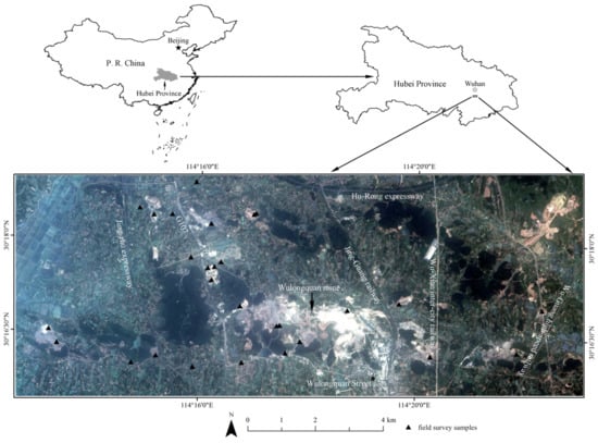
Figure 1.
ZiYuan-3 fused imagery and location of the study area and field samples [12].
Four ZY-3 images within a scene from different cameras on 20 June 2012 were used (Table 1) [12]. Two final data sets were derived with different modals by using some preprocessing methods. First, a 10 m digital terrain model (DTM) was extracted by using two 3.6 m panchromatic (PAN) images based on front- and backward-facing cameras. Then, a 2.1 m multispectral (MS) image was acquired using a pixel-level image fusion method that incorporated Gram–Schmidt spectral sharpening based on the 2.1 m PAN and 5.8 m MS images.

Table 1.
Characteristics of ZiYuan-3 data [12]. PAN: panchromatic; GSD: ground spatial distance; MS: multispectral; NIR: near-infrared.
3. Methods
The basic models of RBM and DBN are explained in Section 3.1. Then, the multimodal and multi-model deep fusion strategy is listed in Section 3.2. Subsequently, Section 3.3 presents some of the methods and data from previous studies. Finally, some metrics and a statistical test method used for the accuracy assessment are introduced in Section 3.4.
3.1. RBM and DBN
3.1.1. Basic Principle of RBM
An RBM network [45,63,64,65] is an energy-based generative NN, i.e., the model reaches the ideal state when the energy is minimal. The RBM network was also used for remote sensing image process tasks [66,67]. It is composed of two layers with binary values (Figure 2), i.e., a visible layer with m nodes v = and a hidden layer with n nodes h = . These two layers are used to input training, validation, and test data and to identify an intrinsic expression of the data. The nodes in different layers are fully connected by symmetric weights (w), and there is a restriction that no intra-layer connections exist. The energy function of an RBM can be calculated:
where = , a = and b = are the bias terms of the corresponding layers and w = {} is the weight between nodes i and j in different layers.
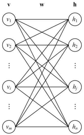
Figure 2.
Schematic diagram of restricted Boltzmann machine [65].
Based on Equation (1), the joint probability distribution of v and h can be obtained as
where is a normalization factor defined as the sum of .
Owing to the conditional independence of the different nodes in each layer, the activation probability for can be calculated as follows when the states of all of the visible nodes are known:
where (x) = 1/(1 + exp(-x)) is the sigmoid activation function. Similarly, the probability for is
An RBM is trained by maximizing the product of the probabilities on a training set or maximizing the expected log probability of one random training sample from the training set. The contrastive divergence algorithm [68] along with Gibbs sampling are used. The change in is given by
where is the learning rate, v represents the reconstructed visible layer (obtained Equation (4)), and h is the updated hidden layer (obtained using Equation (3)), respectively.
The RBM network has an excellent unsupervised learning ability and can fit any discrete distributions when the hidden layer has enough nodes. However, the distributions cannot be effectively calculated [65].
3.1.2. DBN Construction
The DBN was developed based on RBM stacking [45]. It was constructed based on unsupervised pre-training of several RBMs and supervised fine-tuning by using a back propagation (BP) algorithm.
The network structure of the DBN is shown in Figure 3 (taking three RBMs as an example). DBN training is divided into two steps. (1) Pre-training: several RBMs are constructed and stacked to learn deep features (a n-dimensional column vector) of the input data (a m-dimensional column vector), in which the output features of the lower-level RBMs are used as the inputs of the higher-level ones. (2) Fine-tuning: based on the final output layer of the above-mentioned pre-trained network, an activation function (usually softmax) yields an output layer with class probability (a c-dimensional column vector, where c represents the number of class). Afterwards, a BP algorithm is used to update the parameters of the pre-trained network iteratively based on the error of the batch size between the predicted probability vector and the one-hot encoded true labels.
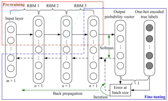
Figure 3.
The structure of deep belief network. RBM: restricted Boltzmann machine.
The layer-wise pre-training ensures that each RBM is optimized and can avoid falling into local optima and long training times. By performing fine-tuning, this contributes substantially to achieving a global optimum. Moreover, only a small set of labeled data is necessary for fine-tuning. Consequently, a robust deep model is obtained.
3.2. Multimodal and Multi-Model Deep Fusion Strategy
In this study, a multimodal and multi-model deep fusion strategy was proposed (Figure 4). DBN has excellent unsupervised learning ability in feature extraction. It can extract deep and discriminative features through unsupervised pre-training of several RBMs. Moreover, a supervised fine-tuning by using a BP algorithm can further learn data-specific features. In particular, the process of fine-tuning has low demand for labeled data, which is suitable for remote sensing image classification tasks. RF and SVM are popular in the remote sensing community and were proved effective for complex open pit mining related landscapes. To take full advantage of the feature extraction and classification abilities of DBN and RF and SVM, this study combined them to develop the DBN-RF and DBN-SVM model. First, multimodal data such as four ZY-3 spectral bands and a DTM were obtained and used to extract numerous low-level spectral–spatial and topographic features. Then, multimodal feature fusion was achieved by stacking the pixel-wise features. The features were subsequently fed to a DBN (taking five RBMs as an example), and the deep features were acquired. Finally, the multi-model deep fusion algorithms DBN-RF and DBN-SVM were achieved by combining the DBN-derived deep features with RF and SVM models. Comparison experiments were conducted using the DBN-S (Section 3.1.2), RF, SVM, FS-RF, and FS-SVM models. The DBN-RF, DBN-SVM, and DBN-S models were developed by using Python software (version 3.5.6), the Keras framework [69], and the Scikit-learn package [70]. The methods employed to optimize the parameters of the DBN and MLAs are described in Section 3.2.1 and Section 3.3.5, respectively. Section 3.2.2 and Section 3.3.3 present the random training, validation, and test sets as well as the independent test set. The low-level multimodal features are explained in Section 3.3.1. The details of the FS method and MLAs are shown in Section 3.3.4 and Section 3.3.5, respectively. The accuracy assessment metrics and statistical tests are described in Section 3.4.
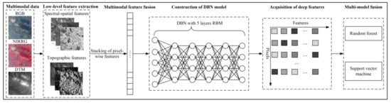
Figure 4.
The framework of multimodal and multi-model deep fusion strategy. RGB: ZiYuan-3 true color image with red, green, and blue bands. NIRRG: ZiYuan-3 false color image with near-infrared, red, and green bands. DTM: digital terrain model. DBN: deep belief network. RBM: restricted Boltzmann machine.
3.2.1. DBN Parameter Optimization
Several parameters affect DBN performance, such as the number of RBM networks (depth), the number of nodes within the hidden layers (node), the activation function, the iteration number (epoch), dropout, and . The first two parameters are the most important and difficult to optimize. Usually, a deeper network or greater number of nodes can yield more informative features and thereby improve the performance. However, a structure that is too complex will lead to a low training efficiency and a longer training time. More seriously, this may lead to over-fitting, and weakening the generalization performance of the model [71].
In this study, the two above-mentioned parameters were optimized. To simplify the parameter optimization process, it was assumed that the number of nodes within the hidden layers were the same (Figure 3).
3.2.2. Training, Validation, and Test Sets
In this study, five groups of training, validation, and test sets were constructed based on a set of data polygons, with 2000, 500, and 500 samples, respectively, for each class (Table 2). The fractions of all of the sets and data polygons are shown in Table 2. The data polygons were collected based on those drawn in Li et al. [12] and using visual interpretation technology. For details, some polygons were added for the mine pit pond, dark road, red roof, and blue roof classes. The polygons for the open pit, ore processing site, and dumping ground classes were completely re-delineated (Table 2) [12]. The three sets were randomly selected from the data polygons and were independent of each other. Some spatial auto-correlations [62] existed. For example, the total pixels of three sets for some classes accounted for over 20% of the corresponding data polygons. The training and validation sets were used for parameter optimization and model development while the test set was employed for an accuracy assessment. In regard to the land covers, see Section 3.3.2. Figure 5a illustrates the schematic diagrams of the training, validation, and test samples, and Figure 5b depicts the spatially independent test samples (for details, see Section 3.3.3).
Table 2.
Number and area of data polygons (DPs) and fractions (%) of training, validation, and test sets. Fraction 1: fraction of pixels in training set and DPs; Fraction 2: fraction of pixels in validation (test) set and DPs; Fraction 3: fraction of pixels in those three sets and DPs.
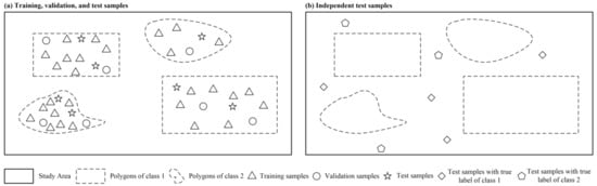
Figure 5.
The schematic diagram of developing training, validation, and test samples and the spatially independent test samples (taking two classes as example).
3.3. Referenced Data and Algorithms
Some data and algorithms were directly obtained from a previous study [12] and are briefly described as follows.
3.3.1. Employed Low-Level Features
Based on the multimodal data, 106 low-level features were extracted [12] and employed in this study (Table 3). First, the spectral–spatial features were derived from the fused MS image by using spectral enhancement (i.e., vegetation index), FR (i.e., principal component analysis), spatial filtering (i.e., Gaussian low-pass, standard deviation, and mean filters), and texture extraction of the gray level co-occurrence matrix. Then, two other topographic features (slope and aspect) were derived from the DTM based on the terrain surface analysis. Multimodal feature fusion was achieved by stacking all of the spectral, spatial, and topographical features. The features were fed to the DBN to identify informative deep features.
Table 3.
Employed low-level features (revised from [12]).
3.3.2. LCC Scheme
This study was focused on the FLCC of CMALs. Consequently, the second-level LCC scheme described in Li et al. [12] was selected. It includes the following: four types of crop land (i.e., paddy, greenhouse, green dry land, and fallow land); four types of forest land (i.e., woodland, shrubbery, coerced forest, and nursery); two water classes (i.e., pond and stream and mine pit pond); three road classes (i.e., dark road, bright road, and light gray road); three types of residential land (i.e., bright roof, red roof, and blue roof); one bare surface land; and three types of open pit mining land (i.e., open pit, ore processing site, and dumping ground).
All of the other procedures, such as the training, validation, and test set construction, FS implementation, deep feature extraction, model development, and accuracy assessment were performed by using the above-mentioned second-level LCC scheme.
3.3.3. Independent Test Set
The independent test set at the first level described by Li et al. [12] (i.e., crop, forest, water, road, residential, bare surface, and open pit mining land) was further tested in this study to examine the reliability of the multimodal and multi-model deep fusion strategy. For each class, 100 pixels were included in the test set. Figure 5b shows that the test set is independent from the data polygons.
3.3.4. FS Method
FS [12] was implemented using the varSelRF package [72] within R software [73] and the feature subsets yielding the lowest out-of-bag errors were selected. For five random training sets, different feature subsets were obtained for subsequent MLA-based classifications.
3.3.5. MLAs for Comparison and Fusion
RF and SVM algorithms were used for comparison and fusion with DBN-derived deep features. For the comparison experiments, the RF and SVM models were developed using the randomForest [74] and e1071 [75] packages in the R platform [73].
The RF algorithm [76] contains an ensemble of numerous CARTs, which usually exhibit a promising performance in remote sensing [77]. The SVM algorithm is also popular in the remote sensing community [78] and is mainly based on structural risk minimization theory and kernel functions [79].
Parameter optimization of the RF and SVM algorithms in the comparison experiments was also conducted using the two above-mentioned packages. For the RF-based models, the parameter ntree was set to the default value of 500. In addition, the parameter mtry should be optimized [77]. First, the training set along with a series of parameter values for mtry were used to train RF-based models. Then, the trained models were used to predict the validation set. Several overall accuracy (OA) values for the validation set were obtained. Finally, the mtry value that resulted in the highest average OA value was the corresponding parameter optimization result. The cost function of RF is Gini index. The kernel of the radial basis function was used for the SVM-based models, and the parameters cost and gamma were optimized [80]. A grid search method and the hinge loss function were used. The combination of cost and gamma values resulting in the highest average OA for the validation test was the corresponding parameter optimization result. For the DBN-RF and DBN-SVM models, the three above-mentioned parameters were also optimized and complemented using Python. The parameters of DBN were first optimized with a grid search method and a cross-entropy cost function. Then the three above-mentioned parameters for RF and SVM were optimized.
3.4. Accuracy Assessment
The accuracy assessment was performed based on five metrics, i.e., the OA, Kappa coefficient, F1-score, F1-measure, and the percentage deviation. The OA and Kappa coefficient were used to evaluate the overall performance of different classification models. The F1-measure is calculated based on the harmonic average of the precision and recall values [81] and was used to evaluate the accuracy for each land cover class. The F1-score is the arithmetic average of all of the F1-measures of different classes and was used to evaluate the average accuracy of all of the land cover types. The percentage deviation [82] was calculated based on the four previous metrics to quantify the performance differences among the different classification models. In addition, a generalized McNemar test [83] suitable for multi-class classification was used to investigate whether there were any significant differences among the models.
4. Results
Figure 6 presents the FS, parameter optimization, and accuracy assessment processes. Based on five groups of training, validation, and test sets (Figure 6a), FS yielded two feature subsets, both with 34 features (Figure 6b, for details see Section 4.1). In the parameter optimization process, only the first group of training and validation sets was used for the DBN-based models (Figure 6(c1)). First, the depth and node were optimized for the DBN-S model using five different random initializations of the DBN (Section 4.2.1). Based on the optimized DBN, the mtry, cost, and gamma parameters were optimized for the DBN-RF and DBN-SVM models (Section 4.2.2). Owing to the randomness of the RF algorithm, five trials were performed to obtain the optimal parameters of the DBN-RF model. Five groups of training and validation sets were used to optimize the MLA-based models (Figure 6(c2), for details see Section 4.2.3). For the RF and FS-RF models, an optimized value of mtry was obtained for each group of data sets based on five random runs. For the SVM and FS-SVM models, the same values of cost and gamma were obtained for all five groups of data sets based on five runs. Because the first and third groups of data sets yielded the same feature subset, the second, fourth, and fifth groups of data sets yielded another one. The parameter optimization of FS-RF is displayed separately for each case in Figure 6(c2). In the model assessment process, five test sets were used (Figure 6d, for details see Section 4.3). In total, there was just one DBN-S, DBN-RF, and DBN-SVM model. However, there were five RF, SVM, FS-RF, and FS-SVM models for five groups of training, validation, and test sets, respectively. Owing to the randomness of the DBN and RF algorithms, each test set yielded five sets of accuracies for the DBN-S, DBN-RF, DBN-SVM, RF, and FS-RF models. Then, the final accuracies of those models were averaged 25 times, and five times for the SVM and FS-SVM models. For the independent test set, some models were used to obtain only a group of accuracies for comparison (Section 4.5).
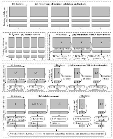
Figure 6.
The used data sets and number of repeated runs in the process of feature selection (FS), parameter optimization, and accuracy assessment. DBN: deep belief network. RF: random forest. SVM: support vector machine. DBN-S: DBN with softmax classifier. DBN-RF: the fused model of DBN and RF. DBN-SVM: the fused model of DBN and SVM. MLAs: machine learning algorithms. FS-RF: RF with FS method. FS-SVM: SVM with FS method.
4.1. Feature Subsets for MLA-Based Classification
Based on the FS procedure, the five random training sets yielded two different feature subsets that had a different feature importance. Training sets 1 and 3 yielded feature subset 1; the average and standard deviation values of the mean decrease in accuracy for each feature were calculated (Figure 7). Training sets 2, 4, and 5 yielded feature subset 2; the average and standard deviation values of the mean decrease in accuracy for each feature were also calculated (Figure 7). Similar to Li et al. [12], about 32% of the features (i.e., 34) were selected for almost all types.
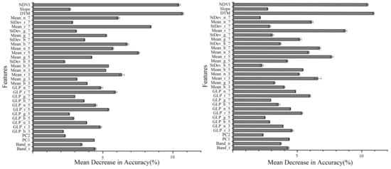
Figure 7.
The average and standard deviation values of mean decrease in accuracy for different features in feature subset 1 (left) and 2 (right). As for features’ name, see Li et al. [12] for detail.
4.2. Parameter Optimization Results
4.2.1. Parameter Optimization for DBN-S
For deep feature extraction using the DBN-S model, two parameters were optimized. The first group of training and validation sets was used, and the process was repeated five times. The depth was set between 1 and 6, and the node was set to one group of values (50, 150, 350, 500, 800, 1500, and 2000). Moreover, to simplify the optimization process, it was assumed that the node was the same in each hidden layer. Meanwhile, the activation function, , epoch, and the mini-batch size were set to sigmoid, 0.0001, 800, and 2048, respectively. The combination of 5 and 1500 was selected for the depth and node (Table 4), which yielded the highest average OA of 94.19% ± 0.39% for validation set 1. The average and standard deviation of the OA for validation set 1 derived from different parameter combinations are depicted in Figure 8.
Table 4.
Parameter optimization results for deep features-based models. DBN-S: deep belief network (DBN) with softmax classifier. DBN-RF: the fused model of DBN and random forest. DBN-SVM: the fused model of DBN and support vector machine.
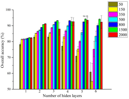
Figure 8.
The average and standard deviation values of overall accuracy for validate set derived from different parameter combinations.
4.2.2. Parameter Optimization for Multi-Model Fusion
For the multi-model fusion of the DBN algorithm and MLAs, the parameters for the MLAs were optimized. With respect to the DBN-RF model, since the optimized value of the node was 1500, the value of mtry ranged from 100 to 1500 in steps of 100. Finally, the optimal value of mtry was determined to be 100 (Table 4), which yielded the highest average OA of 94.22% ± 0.02%.
For the fused DBN-SVM model, cost and gamma were optimized. In total, 48 combinations were used, i.e., eight values () of cost and 10 () of gamma [12]. The optimal parameter combination was determined to be cost = and gamma = (Table 4), which yielded the highest OA of 94.97%.
4.2.3. Parameter Optimization for MLAs
For the MLA-based models, three parameters were optimized. For the RF and FS-RF models, mtry ranged from 1 to 34 and 1 to 106, respectively, in steps of 1. For the SVM and FS-SVM models, the parameter spaces were the same as those described in Section 4.2.2.
With respect to the RF-based models, five repeated runs were performed for each data set to achieve specific parameters. However, for the SVM-based models, five runs were performed for all of the data and the averaged results were used to determine the optimal parameter combinations. As a result, for data sets 1, 2, 3, 4, and 5 with all of the features, the mtry values were 60, 53, 68, 56, and 55, which correspond to average OAs of 88.85% ± 0.09%, 89.49% ± 0.11%, 89.21% ± 0.07%, 89.02% ± 0.09%, and 88.86% ± 0.10%, respectively (Table 5). For those with feature subsets, the optimized values of mtry were 19, 18, 22, 17, and 15, which correspond to average OAs of 89.98% ± 0.06%, 91.05% ± 0.02%, 90.31% ± 0.07%, 90.72% ± 0.05%, and 90.39% ± 0.05%, respectively (Table 5). For all of the data with all of the features, the combination of and for cost and gamma with an accuracy of 78.05% ± 0.47% was achieved (Table 5). For those with feature subsets, the combination of and for cost and gamma with an accuracy of 92.35% ± 0.35% was acquired (Table 5).
Table 5.
Parameter optimization results for machine learning algorithm-based models. RF: random forest. SVM: support vector machine. FS-RF: RF with feature selection (FS) method. FS-SVM: SVM with FS method.
4.3. Accuracy Assessment and Analysis of Five Random Test Sets
4.3.1. Overall Performance
The time of each model based on the first group of training, validation, and test sets presents in Table 6. The long-time of FS-RF and FS-SVM was attributed to the feature selection process, which took 1.93 h. The parameter optimization process needed more time than the model training and prediction. The convergence process diagram of DBN-S depicts in Figure 9. When the iteration number reached 500 the model was stable.
Table 6.
The time (hour) for each model.
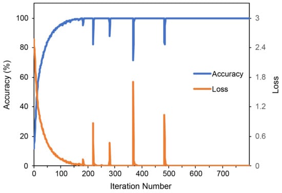
Figure 9.
The convergence process diagram of DBN-S.
The overall performance of the different models based on the OA, Kappa, and F1-score are shown in Table 7. The percentage deviations of the three metrics between the models are presented in Table 8.
Table 7.
Overall performance of different models. RF: random forest. SVM: support vector machine. FS-RF: RF with feature selection (FS) method. FS-SVM: SVM with FS method. DBN-S: deep belief network (DBN) with softmax classifier. DBN-RF: the fused model of DBN and RF. DBN-SVM: the fused model of DBN and SVM.
Table 8.
The percentage deviation values (%) of overall accuracy, Kappa, F1-score between different models. RF: random forest. SVM: support vector machine. FS-RF: RF with feature selection (FS) method. FS-SVM: SVM with FS method. DBN-S: deep belief network (DBN) with softmax classifier. DBN-RF: the fused model of DBN and RF. DBN-SVM: the fused model of DBN and SVM.
For the MLA-based models, the OA decreased in the order of 91.77% ± 0.57% (FS-SVM), 90.39% ± 0.42% (FS-RF), 88.90% ± 0.20% (RF), and 77.88% ± 0.53% (SVM). The order is the same for Kappa and the F1-score. The best model was determined to be the FS-SVM model. It is clear that FS improved the classification accuracy. After FS, the OA, Kappa, and F1-score improvements of 1.68%, 1.79%, and 1.69%, respectively, were achieved for the RF-based model (Table 8). Compared to the SVM model, the FS-SVM model considerably improved the OA, Kappa, and the F1-score, by 17.84%, 19.06%, and 17.95%, respectively (Table 8). For the models based on all of the features, the RF model was better than the SVM model, yielding improvements of 14.15%, 15.11%, and 14.22% in the OA, Kappa, and the F1-score, respectively (Table 8). However, for the models based on feature subsets, the FS-SVM model slightly outperformed the FS-RF model (Table 8).
For the deep feature-based models, the OA decreased in the order of 94.74% ± 0.35% (DBN-SVM), 94.23% ± 0.67% (DBN-S), and 94.07% ± 0.34% (DBN-RF). The order is the same for Kappa and the F1-score. The best model was determined to be the DBN-SVM. Moreover, after model fusion, improvements of 0.54%, 0.56%, and 0.53% were achieved in the OA, Kappa, and the F1-score, respectively (Table 8). However, compared with the DBN-S model, the DBN-RF model slightly decreased the classification accuracies (Table 8).
Compared to the best MLA-based model, the FS-SVM model, all of the deep feature-based models yielded higher classification accuracies. The DBN-S model yielded improvements of 2.60%, 2.76%, and 2.60% in the OA, Kappa, and the F1-score, respectively (Table 8). The improvements for the OA, Kappa, and the F1-score were 2.46%, 2.59%, and 2.46% when the DBN-RF model was used and 3.15%, 3.33%, and 3.15% when the DBN-SVM model was employed, respectively. (Table 8).
4.3.2. Class-Specific Performance
The class-specific performance of the different models based on the F1-measure are displayed in Table 9. The percentage deviations between the models are shown in Table 10.
Table 9.
F1-measure values (%) for different land covers obtained by different classification models. RF: random forest. SVM: support vector machine. FS-RF: RF with feature selection (FS) method. FS-SVM: SVM with FS method. DBN-S: deep belief network (DBN) with softmax classifier. DBN-RF: the fused model of DBN and RF. DBN-SVM: the fused model of DBN and SVM.
Table 10.
The percentage deviation values (%) of F1-measures for different land covers obtained between different classification models. RF: random forest. SVM: support vector machine. FS-RF: RF with feature selection (FS) method. FS-SVM: SVM with FS method. DBN-S: deep belief network (DBN) with softmax classifier. DBN-RF: the fused model of DBN and RF. DBN-SVM: the fused model of DBN and SVM. A – I: RF vs. SVM, FS-RF vs. RF, FS-SVM vs. SVM, FS-SVM vs. FS-RF, DBN-S vs. FS-SVM, DBN-RF vs. FS-SVM, DBN-SVM vs. FS-SVM, DBN-RF vs. DBN-S, and DBN-SVM vs. DBN-S, respectively.
For the F1-measures for almost all of the classes, the performance of the MLA-based models (Table 9) decreased in an order that agrees with the conclusion drawn in Section 4.3.1. There are only three exceptions: for woodland, shrubbery, and ore processing site, the FS-RF model outperformed the FS-SVM model (i.e., the percentage deviations are negative in column D of Table 10). Similarly, for the F1-measures of almost all of the classes, the performance of the deep feature-based models (Table 9) decreased in an order that agrees with the conclusion drawn in Section 4.3.1 with only five exceptions. For fallow land, woodland, shrubbery, pond and stream, and mine pit pond, the DBN-RF model outperformed the DBN-S model (i.e., the percentage deviations are positive in column H of Table 10). For the F1-measures of all of the classes, all of the deep feature-based models outperformed the best MLA-based model, i.e., the FS-SVM model (Table 9).
For the highest F1-measure of each land cover type derived from the MLA-based models, most achieved an accuracy over 90% (Table 9), i.e., paddy, greenhouse, coerced forest, nursery, pond and stream, mine pit pond, dark road, bright road, red roof, blue roof, bare surface, open pit, and dumping ground. Only six and one classes achieved over 80% and 70% accuracy, respectively (Table 9), i.e., green dry land, fallow land, woodland, shrubbery, light gray road, and ore processing site and bright roof. For the highest F1-measure of each land cover type derived from the deep feature-based models, almost all of the classes achieved over 90% accuracy and only three over 80% (Table 9), i.e., fallow land, shrubbery, and bright roof.
The percentage deviations between the RF and SVM models for the different types of land cover are presented in column A of Table 10. As demonstrated in Table 10, the RF algorithm significantly outperformed the SVM algorithm. The percentage deviations range from 1.40% to 29.61% with an average of 15.39%. Moreover, 60% of the land cover types exhibited over 10% deviation, i.e., green dry land, fallow land, woodland, shrubbery, nursery, pond and stream, light gray road, bright roof, bare surface, open pit, ore processing site, and dumping ground.
FS resulted in positive effects for the accuracies of all of the classes (columns B and C of Table 10). For the RF-based models, the percentage deviations range from 0.28% to 3.27% with an average of 1.73%. However, for the SVM-based models, the percentage deviations are very large, ranging from 4.63% to 36.90% with an average of 19.19%. Moreover, 75% of the land cover types exhibited over 10% deviation, i.e., paddy, green dry land, fallow land, woodland, shrubbery, coerced forest, nursery, pond and stream, mine pit pond, light gray road, bright roof, bare surface, open pit, ore processing site, and dumping ground.
In general, the FS-SVM model outperformed the FS-RF model for almost all of the land cover types (column D of Table 10). Only three exceptions exist, i.e., woodland (−0.69%), shrubbery (−0.47%), and the mineral processing site (−0.70%). For the other classes, the percentage deviations range from 0.11% to 4.43% with an average of 1.94%.
For all of the classes, the percentage deviations between all the deep feature-based models and the FS-SVM model are positive (columns E–G of Table 10). For the DBN-S, DBN-RF, and DBN-SVM models, the percentage deviations range from 0.11% to 9.69% with an average of 2.79%, from 0.17% to 8.61% with an average of 2.61%, and from 0.19% to 10.38% with an average of 3.36%, respectively.
Among the deep feature-based models, the DBN-S model outperformed the DBN-RF model for almost all of the classes (column H of Table 10). Also, the DBN-SVM model outperformed the DBN-S model for all of the classes (column I of Table 10). For the percentage deviations between the DBN-RF and DBN-S models, only five exceptions exist, i.e., fallow land (0.11%), woodland (0.23%), shrubbery (0.05%), pond and stream (0.04%), and mine pit pond (0.06%). For the other classes, the percentage deviations range from −0.98% to −0.10% with an average of −0.27%. Meanwhile, the percentage deviations between the DBN-SVM and DBN-S models range from 0.07% to 1.12% with an average of 0.55%.
4.3.3. Statistical Tests
Statistical tests were performed on the pairs of results predicted for test set 1 using seven models. For the RF and DBN-based models, results with OAs closer to the average values of five random runs were selected. For the SVM and FS-SVM models, the individual results were directly used (Table 11). Table 12 shows the chi-square and p values between the different models. If the chi-square value is greater than 30.14, a statistical significance exists at the 95% confidence level (p < 0.05). The statistical tests revealed the following. (1) The RF algorithm was significantly better than the SVM algorithm (with chi-square and p values of 89.14 and 0.00, respectively). (2) FS had different effects on different algorithms. There was no significant difference between the FS-RF and RF algorithms (with a p value of 0.15); however, a significant difference was observed between the FS-SVM and SVM algorithms, with chi-square and p values of 46.21 and 0.00, respectively. (3) Although the average OA difference between the FS-SVM and FS-RF algorithms was not large, a significant difference was observed (with chi-square and p values of 55.94 and 0.00, respectively). (4) All the deep feature-based models significantly outperformed the best MLA-based model, i.e., the FS-SVM model. (5) Among the three deep models, the fused DBN-SVM model significantly outperformed the DBN-S model (with chi-square and p values of 31.70 and 0.03, respectively), and there was no significant difference between the DBN-S and DBN-RF models, (with chi-square and p values of 25.57 and 0.14, respectively).
Table 11.
Averaged overall accuracies (OAs) and those closer to those of Test 1 based on different models. RF: random forest. SVM: support vector machine. FS-RF: RF with feature selection (FS) method. FS-SVM: SVM with FS method. DBN-S: deep belief network (DBN) with softmax classifier. DBN-RF: the fused model of DBN-RF. DBN-SVM: the fused model of DBN and SVM.
Table 12.
The percentage deviation values (%) of overall accuracy, Kappa, F1-score between different models. RF: random forest. SVM: support vector machine. FS-RF: RF with feature selection (FS) method. FS-SVM: SVM with FS method. DBN-S: deep belief network (DBN) with softmax classifier. DBN-RF: the fused model of DBN and RF. DBN-SVM: the fused model of DBN and SVM.
4.4. Visual Assessment of Predicted Maps
For the CMAL, the FLCC map predicted based on the DBN-SVM model and the LCC maps based on the DBN-SVM and FS-RF models [12] are illustrated in Figure 10. The LCC map that predicted by using the DBN-SVM model was derived by grouping the FLCC results into seven first-level classes. The LCC map that predicted based on the FS-RF model was obtained from [12]. Some classes in the LCC results derived from the FS-RF model are superior to those from the DBN-SVM model. The main differences are the misclassification of roads, residential land, and bare surfaces as open pit mining land. Besides the spectral similarity among those land cover types, two main factors caused those differences. (1) The training samples for open pit mining land in [12] were randomly selected from all the open pit mining land in the study area; however, the samples used in this study were obtained from a very small subset of all of the open pit mining land (Table 2). Consequently, the spatial auto-correlation [62] significantly contributed to the results obtained using the FS-RF model [12]. (2) Compared to the FS-RF model, the DBN-SVM model normalized the stacked multimodal features. This might have weakened the advantages of the topographic information and resulted in misclassification of the above-mentioned land cover types. The other classes such as water, crop land, and forest land were classified better in the LCC map derived from DBN-SVM.
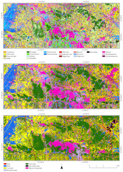
Figure 10.
The predicted maps of fine land cover classification (LCC) based on the fused model of deep belief network and support vector machine (DBN-SVM), and LCC based on DBN-SVM and random forest with feature seleciton method [12] (from top to bottom).
For the FLCC, besides the misclassification of the above-mentioned first-level classes, there was misclassification within some second-level classes. For example, many pond and stream pixels were incorrectly classified as mine pit pond pixels. In addition, many dumping ground and ore processing site pixels were misclassified as open pit pixels. These misclassifications were also attributed to the two above-mentioned factors.
4.5. Accuracy Assessment and Statistical Tests for Independent Test Set
For the independent test set, the best MLA-based model in [12] was the FS-RF model with an OA of 77.57%. Among the DBN-based models, the DBN-S and DBN-SVM models were further examined. Their OAs are shown in Table 13. Statistical tests were also performed and Table 14 shows the resulting chi-square and p values. In this situation, if the chi-square value is greater than 12.59, a statistical significance exists at the 95% confidence level (p < 0.05).
Table 13.
Overall accuracy (OA) (%) for independent test set. FS-RF: random forest with feature selection method. DBN-S: deep belief network (DBN) with softmax classifier. DBN-SVM: the fused model of DBN and support vector machine.
Table 14.
The chi-square and p values based on independent test set between different models. FS-RF: random forest with feature selection method. DBN-S: deep belief network (DBN) with softmax classifier. DBN-SVM: the fused model of DBN and support vector machine.
Obviously, the DBN-S and DBN-SVM models significantly outperformed the FS-RF model with OAs of 79.86% and 81.14% and improvements of 2.95% and 4.60%, respectively. Although there was a 1.60% deviation between the DBN-SVM and DBN-S models, no significant difference existed between them.
5. Discussion
5.1. Effectiveness of the Multimodal and Multi-Model Deep Fusion Strategy
The results in Section 4.3 indicate that the multimodal and multi-model deep fusion strategy was very effective for FLCC of CMAL. In particular, the DBN-SVM model significantly outperformed the MLA-based models with the multimodal low-level features and the deep feature-based DBN-S model. Moreover, the DBN-RF model was also significantly better than the MLA-based models and had a predictive power similar to the DBN-S model. The results in Section 4.5 also prove that the multimodal and multi-model deep fusion strategy was effective for LCC of CMAL. The DBN-SVM model significantly outperformed the FS-RF model and was slightly better than the DBN-S model.
Some previous studies involving DBN-based models yielded similar conclusions. For example, Zhong et al. [57] indicated that the DBN-CRF model performed significantly better than the SVM, CRF, CNN, and DBN-LR models. Chen et al. [47] proved that the DBN-LR model was significantly better than the SVM and extended the morphological profile-based SVM models. Le et al. [58] also showed that the DBN-LR model was superior to the SVM model. Ayhan and Kwan [59] developed the following conclusions. (1) The DBN model was slightly better than the SVM model when spectral information was employed. (2) The DBN model was better than the SAM-based models. (3) Finally, DBN model was slightly worse than the SVM model when spectral–spatial information was used. Qin et al. [60] revealed that the RBM-AdaBoost model performed better than the single and stacked RBM, RBM-based nearest neighbor, RBM-based bagging, minimum distance, nearest neighbor, Wishart, and RF models. In addition, Qin et al. [60] demonstrated that the RBM-based nearest neighbor and bagging models performed better than the other models. He et al. [61] revealed that the DSN-LR model was better than the SVM and single-layer NN-based LR models. In summary, fused models based on DBNs are effective for various classification tasks.
There have also been some studies involving CNN-based multimodal and multi-model fusion strategies. For example, Chen et al. [84] fused multi-/hyperspectral and LiDAR data and CNN and LR models. The results showed that the fused model significantly outperformed other SVM-based models. Li et al. [85] fused hyperspectral and LiDAR data and CNN, SVM, and extreme learning machine (ELM) models. The results again demonstrated that the fused model performed better than various SVM and ELM-based models. Overall, multimodal and multi-model deep fusion strategies based on different data and algorithms might be effective for the LCC of complex landscapes, which may be worth exploring further.
In addition, it is worth noting that Zhong et al. [57], Chen et al. [47], Le et al. [58], and Chen et al. [84] used end-to-end training for multi-model fusion. However, Qin et al. [60], He et al. [61], and Li et al. [85] first trained the DL model and then fused it with MLAs, which was also done in this study. End-to-end training might yield more effective models; however, it is more complex and requires more time. Meanwhile, separate training using DL algorithms as feature extractors is easy to implement. Both methods should be investigated further in different situations.
The analysis of the predicted maps also revealed that more effective methods of fusing multimodal low-level features before feeding them to DL models should be further investigated to take advantage of topographic information.
In general, the proposed strategy had some limitations. These limitations include: (1) there are many parameters that need to be optimized; (2) the issue of exploring the DBN-based deep features; (3) it required many low-level features and deep features cannot be learned end-to-end; (4) the developed deep features might be poorer than CNN-based ones; and (5) the temporal-space applicability needs to be further verified. If the strategy was applied in other areas or with images from different seasons, the strategy does not need to be changed; however, the LCC scheme, training data, and parameters should be updated. In theory, the corresponding accuracies would not be significantly reduced when the LCC scheme and parameters were reasonable and the training data was reliable. For example, when using an image in February, the four crop lands were indistinguishable whether based on visual interpretation or classification algorithms. As a result, the LCC scheme should be adjusted. Of course, multi-temporal images (e.g., in February and June) might help improve the performance of the proposed strategy with the same LCC scheme in this study.
5.2. Effects of Sampling Design
There are generally three methods of dividing data sets: the hold-out; cross-validation; and bootstrap methods. The hold-out approach is the most common in remote sensing. Spatial features have been considered to provide important information for remote sensing classification [12,47,85] owing to the spatial auto-correlation [62]. Consequently, some modifications were made to the hold-out method. In this study, the hold-out was employed to construct training, validation, and test sets (Figure 5a); however, most of the samples were not used (at least 70%, for details see Table 2). Moreover, the independent test set (Figure 5b) was derived using a more specialized hold-out method.
The common sampling designs used in remote sensing are shown in Figure 11, which used training and test samples with a proportion of 9:1 as an example. Another sampling design used equal amounts of training pixels for each class and the remaining were used as test pixels (e.g., [57,84]). In addition, arbitrary numbers of training and test samples could be selected (e.g., [85]). These two sampling designs have similar principles to that in Figure 11 and they were not discussed here. Figure 11a shows the situation in which 90% of the pixels were selected for training while the remaining 10% were used for testing. This approach is often used for classification based on a benchmark with ground truth. This sampling design is generally employed in hyperspectral classification, such as in [47,58,59,60,61]. However, the spatial auto-correlation [62] between the training and test samples might contribute to the classification [12,62], which makes the classification accuracy inordinately high. Figure 11b depicts the situation in which the pixels that selected as the training and test samples had a proportion of 9:1. The spatial auto-correlation [62] between the training and test samples here is weaker than in Figure 11a. Consequently, this design could be more reasonable for achieving an objective classification accuracy assessment. However, it might result in limited training samples not suitable for DL-based models, which is worth investigating. Figure 11c presents the situation in which 90% of the pixels of data polygons were selected as training samples and the remaining 10% were used as test samples. This division is often used for the classification of large-scale study areas with no ground truth. The data polygons were manually delineated to sample the training and test sets. As demonstrated in Figure 11a, all of the labeled data was used, which resulted in a strong spatial auto-correlation [62]. Figure 11d shows the situation in which the pixels in the data polygons were divided into training and test samples with a proportion of 9:1. Again, this case is more reasonable than that shown in Figure 11c. Figure 11e depicts the situation in which the pixels inside and outside the data polygons were selected as training and test samples, respectively, with a proportion of 9:1. This design may be the most reasonable because the training and test samples are spatially independent. However, the labels of the test samples must be determined manually and individually.
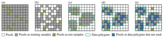
Figure 11.
Different sampling designs of training and test samples (taking the proportion of 9:1 as example).
The high accuracies for the test sets were partly attributed to the spatial auto-correlation [62] of the training, validation, and test samples derived using the design shown in Figure 11d. However, the effect was very slight. The data in Table 2 indicates that only 12.88% of the pixels in the data polygons on average were used to construct the training, validation, and test sets for each class. The relatively low accuracies of the independent test sets were due to the fact that there was almost no spatial auto-correlation [62] between the training sets and independent test sets (Figure 11e). The analysis of the predicted maps also proves the effect of the spatial auto-correlation [62].
Taking the results of the DBN-SVM model as an example, there were six classes with accuracies between 90% and 95%. The percentage of pixels used in the data polygons ranged from 2.44% to 26.09% with an average and standard deviation of 10.74% ± 8.03%. In particular, there were five classes with less than 3% of the pixels in the data polygons used, among which the accuracies of three classes were less than 90%, and the other two were 92.01% ± 0.61% and 97.26% ± 0.34%. These results indicate that the effect of the spatial auto-correlation [62] was slight and that the accuracies for the different types of land cover mainly depends on the classification algorithm and separability of the land cover types.
It can be concluded that the spatial auto-correlation [62] should be controlled at a normal degree. Consequently, the sampling design selection depends on the specific application and research objective. Taking the classification of a large study area as an example, if the aim is to compare classification algorithms, it seems that any of the designs shown in Figure 11c–e could be used. Of course, the design presented in Figure 11d is optimal in this situation. However, if the objective is to obtain good classification maps, the design shown in Figure 11e may be effective and the training samples should be added to take full advantage of the effect of the spatial auto-correlation [62].
5.3. Effects of FS and Parameter Optimization
Regarding the effects of FS, conclusions can be drawn from this study that are similar to those of previous studies. (1) The results in Section 4.3.2 reveal that the land cover types with a higher separability (i.e., higher F1-measures) were less sensitive to FS [12,82] (i.e., their F1-measures deviated less). (2) FS significantly improved the classification performance [12,30], i.e., the FS-based SVM model significantly outperformed SVM algorithm. (3) The SVM model was more sensitive to FS than the RF model [12,29,86], i.e., the FS-SVM method exhibited greater improvements than the FS-RF approach.
Parameter optimization was indispensable, especially for the DL-based models. Ayhan and Kwan [59] concluded that one of the main reasons that the DBN model did not perform better than the SVM-based spectral–spatial model was that the parameters of the DBN model were directly given (two RBMs with 200 hidden units); hence, the resulting model was too simple. In this study, the depth and node were jointly optimized in the DBN model. In most similar studies, at least one of these two parameters are optimized. For example, Chen et al. [47] optimized the depth and fixed node. Le et al. [58] optimized the node and epoch, and fixed depth. Qin et al. [60] optimized the node in the RBM-AdaBoost model. He et al. [61] optimized the depth and dropout, and fixed the node. All of these studies proved the superiority of DBN-based models. There have also been studies in which the parameters of the DBN and DBN-based model were not optimized and a better performance was achieved. For example, Zhong et al. [57] fixed the depth and node in the DBN-CRF model to 3 and 50, respectively, and the fused model performed better. This finding could further prove the effectiveness of the DBN approach.
In addition, the end-to-end training of the DL-based fused model involved more parameters. Consequently, the selection of the parameters to be optimized and how to optimize them are very important topics and are worth exploring further for multi-model deep fusion methods. In particular, the meta-heuristic algorithms may be positive.
5.4. Selection of Statistical Test Method and Effects of Test Set Size
Statistical tests are important and useful for comparing classification algorithms. In particular, they can elucidate whether two algorithms have a statistically significant difference. In some of the above-mentioned studies involving DL-based fused models, statistical tests were performed. For example, Zhong et al. [57] and Chen et al. [84] used the McNemar test method [87]. Chen et al. [47] performed a paired t-test [88]. McNemar tests were used in some other studies, such as those described in Duro et al. [89], Li et al. [12], Li et al. [90,91], and Maxwell et al. [31]. In addition, a Mann–Whitney U-test [92] was used by Fassnacht et al. [93]. It is worth noting that the McNemar test [87] is designed for two-class classification, while the other two tests are intended for multi-class classification. Because the McNemar test [87] is easy to implement compared to the t- and U-tests [88,92], it is also widely used for multi-class classification with relative reasonable results, such as in the above-mentioned studies [12,31,57,84,89,90,91]. However, when the test set is large, this method is not applicable. For example, Li et al. [12] performed fine classification of three open pit mining land covers with a test set containing 883264 pixels. The results of the McNemar test were not reasonable. Moreover, Duro et al. [89] revealed that if the test set is too small, it is not sufficient to obtain reasonable results. In this study, a generalized McNemar test [83] suitable for multi-class classification was selected. In addition, for the FLCC of a CMAL with a relatively large test set and multiple classes, the results are reasonable. However, for the independent test set, the results indicate that the DBN-SVM model is slightly better than the DBN-S model. This finding might be attributable to the small size of the independent test set. In summary, the generalized McNemar test [83] with a relatively large test set is recommended for comparing classification algorithms.
6. Conclusions
A multimodal and multi-model deep fusion strategy was proposed and tested by conducting FLCC of a CMAL in Wuhan City, China in this study. Three steps were performed. (1) Low-level multimodal features involving spectral–spatial and topographic information were extracted from ZY-3 imagery and fused. (2) These features were entered into a DBN for deep feature learning. (3) The developed deep features were fed to the RF and SVM algorithms for classification. The fused DBN-RF and DBN-SVM models were compared to the DBN-S, RF, SVM, FS-RF, and FS-SVM models. Parameter optimization, model construction, and accuracy assessment were conducted using two sets of data: five groups of training, validation, and test sets with some spatial auto-correlations and a spatially independent test set. Five metrics, i.e., the OA, Kappa coefficient, F1-measure, F1-score, and percentage deviation, were calculated. Generalized McNemar tests were performed to evaluate the performance of the different models. The results showed the following. (1) In the FLCC of the CMAL, the DBN-SVM model achieved an OA of 94.74% ± 0.35% and significantly outperformed the MLA-based models and deep feature-based model of DBN-S. Moreover, the DBN-RF model was significantly better than the MLA-based models and had a predictive power similar to the DBN-S model. (2) In the LCC of the CMAL, the DBN-SVM model achieved an OA of 81.14%, which significantly outperformed the FS-RF model and was slightly better than the DBN-S model. (3) The FLCC and LCC maps had an acceptable visual accuracy.
The following conclusions were drawn from this study. (1) The multimodal and multi-model deep fusion strategy takes advantage of the low-level and multimodal features, unsupervised learning, and the classification abilities of MLAs is effective for FLCC of CMALs. (2) FS is effective for the MLAs and parameter optimization is indispensable for the MLA- and DL-based models. (3) The sampling design should be properly selected and training samples should be added to take full advantage of the effects of the spatial auto-correlation to obtain better predicted maps of large areas. (4) The generalized McNemar test with a relatively large test set is applicable for comparing classification algorithms. Future work will focus on other fusion methods involving different DL algorithms and MLAs for the FLCC of various complex landscapes.
Author Contributions
Conceptualization, X.L. and W.C.; Data curation, Z.T.; Formal analysis, X.L.; Funding acquisition, X.L. and W.C.; Investigation, Z.T.; Methodology, X.L. and W.C.; Project administration, X.L.; Resources, X.L.; Software, Z.T.; Supervision, W.C. and L.W.; Validation, X.L.; Visualization, X.L. and Z.T.; Writing—original draft, X.L. and W.C.; Writing—review & editing, X.L. and L.W.
Funding
This work was jointly supported by Natural Science Foundation of China (No. 41701516, U1803117, and U1711266 ), the Fundamental Research Funds for Central Universities, China University of Geosciences (Wuhan) (No. CUG170648), and Open Research Project of the Hubei Key Laboratory of Intelligent Geo-Information Processing (No. KLIGIP-2018B07).
Conflicts of Interest
The authors declare no conflict of interest.
References
- DeFries, R.S.; Belward, A.S. Global and regional land cover characterization from satellite data: An introduction to the Special Issue. Int. J. Remote Sens. 2000, 21, 1083–1092. [Google Scholar] [CrossRef]
- Cihlar, J. Land cover mapping of large areas from satellites: Status and research priorities. Int. J. Remote Sens. 2000, 21, 1093–1114. [Google Scholar] [CrossRef]
- Chen, J.; Chen, J.; Liao, A.; Cao, X.; Chen, L.; Chen, X.; He, C.; Han, G.; Peng, S.; Lu, M. Global land cover mapping at 30 m resolution: A POK-based operational approach. ISPRS J. Photogramm. Remote Sens. 2015, 103, 7–27. [Google Scholar] [CrossRef]
- Gong, P.; Wang, J.; Yu, L.; Zhao, Y.; Zhao, Y.; Liang, L.; Niu, Z.; Huang, X.; Fu, H.; Liu, S. Finer resolution observation and monitoring of global land cover: First mapping results with Landsat TM and ETM+ data. Int. J. Remote Sens. 2013, 34, 2607–2654. [Google Scholar] [CrossRef]
- Sellers, P.J.; Meeson, B.W.; Hall, F.G.; Asrar, G.; Murphy, R.E.; Schiffer, R.A.; Bretherton, F.P.; Dickinson, R.E.; Ellingson, R.G.; Field, C.B. Remote sensing of the land surface for studies of global change: Models—Algorithms—Experiments. Remote Sens. Environ. 1995, 51, 3–26. [Google Scholar] [CrossRef]
- Lv, Q.; Dou, Y.; Niu, X.; Xu, J.; Li, B. Classification of land cover based on deep belief networks using polarimetric RADARSAT-2 data. In Proceedings of the 2014 IEEE International Geoscience and Remote Sensing Symposium (IGARSS), Quebec City, QC, Canada, 13–18 July 2014; pp. 4679–4682. [Google Scholar]
- Maxwell, A.E.; Warner, T.A. Differentiating mine-reclaimed grasslands from spectrally similar land cover using terrain variables and object-based machine learning classification. Int. J. Remote Sens. 2015, 36, 4384–4410. [Google Scholar] [CrossRef]
- Myint, S.W.; Gober, P.; Brazel, A.; Grossman-Clarke, S.; Weng, Q. Per-pixel vs. object-based classification of urban land cover extraction using high spatial resolution imagery. Remote Sens. Environ. 2011, 115, 1145–1161. [Google Scholar] [CrossRef]
- Senf, C.; Leitão, P.J.; Pflugmacher, D.; van der Linden, S.; Hostert, P. Mapping land cover in complex Mediterranean landscapes using Landsat: Improved classification accuracies from integrating multi-seasonal and synthetic imagery. Remote Sens. Environ. 2015, 156, 527–536. [Google Scholar] [CrossRef]
- Silveyra Gonzalez, R.; Latifi, H.; Weinacker, H.; Dees, M.; Koch, B.; Heurich, M. Integrating LiDAR and high-resolution imagery for object-based mapping of forest habitats in a heterogeneous temperate forest landscape. Int. J. Remote Sens. 2018, 39, 8859–8884. [Google Scholar] [CrossRef]
- Yan, W.Y.; Shaker, A.; El-Ashmawy, N. Urban land cover classification using airborne LiDAR data: A review. Remote Sens. Environ. 2015, 158, 295–310. [Google Scholar] [CrossRef]
- Li, X.; Chen, W.; Cheng, X.; Wang, L. A comparison of machine learning algorithms for mapping of complex surface-mined and agricultural landscapes using ZiYuan-3 stereo satellite imagery. Remote Sens. 2016, 8, 514. [Google Scholar] [CrossRef]
- Chen, W.; Li, X.; He, H.; Wang, L. A review of fine-scale land use and land cover classification in open-pit mining areas by remote sensing techniques. Remote Sens. 2018, 10, 15. [Google Scholar] [CrossRef]
- Chen, W.; Li, X.; He, H.; Wang, L. Assessing Different Feature Sets’ Effects on Land Cover Classification in Complex Surface-Mined Landscapes by ZiYuan-3 Satellite Imagery. Remote Sens. 2018, 10, 23. [Google Scholar] [CrossRef]
- Ross, M.R.; McGlynn, B.L.; Bernhardt, E.S. Deep impact: Effects of mountaintop mining on surface topography, bedrock structure, and downstream waters. Environ. Sci. Technol. 2016, 50, 2064–2074. [Google Scholar] [CrossRef]
- Wei, L.; Zhang, Y.; Zhao, Z.; Zhong, X.; Liu, S.; Mao, Y.; Li, J. Analysis of Mining Waste Dump Site Stability Based on Multiple Remote Sensing Technologies. Remote Sens. 2018, 10, 2025. [Google Scholar] [CrossRef]
- Johansen, K.; Erskine, P.D.; McCabe, M.F. Using unmanned aerial vehicles to assess the rehabilitation performance of open cut coal mines. J. Clean. Prod. 2019, 209, 819–833. [Google Scholar] [CrossRef]
- Yu, L.; Xu, Y.; Xue, Y.; Li, X.; Cheng, Y.; Liu, X.; Porwal, A.; Holden, E.J.; Yang, J.; Gong, P. Monitoring surface mining belts using multiple remote sensing datasets: A global perspective. Ore Geol. Rev. 2018, 101, 675–687. [Google Scholar] [CrossRef]
- Chen, G.; Li, X.; Chen, W.; Cheng, X.; Zhang, Y.; Liu, S. Extraction and application analysis of landslide influential factors based on LiDAR DEM: A case study in the Three Gorges area, China. Nat. Hazards 2014, 74, 509–526. [Google Scholar] [CrossRef]
- Song, W.; Wang, L.; Xiang, Y.; Zomaya, A.Y. Geographic spatiotemporal big data correlation analysis via the Hilbert–Huang transformation. J. Comput. Syst. Sci. 2017, 89, 130–141. [Google Scholar] [CrossRef]
- Xu, D.; Ma, Y.; Yan, J.; Liu, P.; Chen, L. Spatial-feature data cube for spatiotemporal remote sensing data processing and analysis. Computing 2018, 1–15. [Google Scholar] [CrossRef]
- Zhao, J.; Zhong, Y.; Jia, T.; Wang, X.; Xu, Y.; Shu, H.; Zhang, L. Spectral-spatial classification of hyperspectral imagery with cooperative game. ISPRS J. Photogramm. Remote Sens. 2018, 135, 31–42. [Google Scholar] [CrossRef]
- Tang, C.; Chen, J.; Liu, X.; Li, M.; Wang, P.; Wang, M.; Lu, P. Consensus learning guided multi-view unsupervised feature selection. Knowl.-Based Syst. 2018, 160, 49–60. [Google Scholar] [CrossRef]
- Schmitt, M.; Zhu, X.X. Data fusion and remote sensing: An ever-growing relationship. IEEE Geosci. Remote Sens. Mag. 2016, 4, 6–23. [Google Scholar] [CrossRef]
- Luo, H.; Liu, C.; Wu, C.; Guo, X. Urban change detection based on dempster–shafer theory for multitemporal very high-resolution imagery. Remote Sens. 2018, 10, 980. [Google Scholar] [CrossRef]
- Dalla Mura, M.; Prasad, S.; Pacifici, F.; Gamba, P.; Chanussot, J.; Benediktsson, J.A. Challenges and opportunities of multimodality and data fusion in remote sensing. Proc. IEEE 2015, 103, 1585–1601. [Google Scholar] [CrossRef]
- Gómez-Chova, L.; Tuia, D.; Moser, G.; Camps-Valls, G. Multimodal classification of remote sensing images: A review and future directions. Proc. IEEE 2015, 103, 1560–1584. [Google Scholar] [CrossRef]
- Hui, Z.; Hu, Y.; Yevenyo, Y.Z.; Yu, X. An improved morphological algorithm for filtering airborne LiDAR point cloud based on multi-level kriging interpolation. Remote Sens. 2016, 8, 35. [Google Scholar] [CrossRef]
- Li, X.; Cheng, X.; Chen, W.; Chen, G.; Liu, S. Identification of forested landslides using LiDar data, object-based image analysis, and machine learning algorithms. Remote Sens. 2015, 7, 9705–9726. [Google Scholar] [CrossRef]
- Maxwell, A.E.; Warner, T.A.; Strager, M.P.; Pal, M. Combining RapidEye satellite imagery and Lidar for mapping of mining and mine reclamation. Photogramm. Eng. Remote Sens. 2014, 80, 179–189. [Google Scholar] [CrossRef]
- Maxwell, A.E.; Warner, T.A.; Strager, M.P.; Conley, J.F.; Sharp, A.L. Assessing machine-learning algorithms and image-and lidar-derived variables for GEOBIA classification of mining and mine reclamation. Int. J. Remote Sens. 2015, 36, 954–978. [Google Scholar] [CrossRef]
- Ball, J.E.; Anderson, D.T.; Chan, C.S. Comprehensive survey of deep learning in remote sensing: Theories, tools, and challenges for the community. J. Appl. Remote Sens. 2017, 11, 042609. [Google Scholar] [CrossRef]
- Zhang, L.; Zhang, L.; Du, B. Deep learning for remote sensing data: A technical tutorial on the state of the art. IEEE Geosci. Remote Sens. Mag. 2016, 4, 22–40. [Google Scholar] [CrossRef]
- Zhu, X.X.; Tuia, D.; Mou, L.; Xia, G.S.; Zhang, L.; Xu, F.; Fraundorfer, F. Deep learning in remote sensing: A comprehensive review and list of resources. IEEE Geosci. Remote Sens. Mag. 2017, 5, 8–36. [Google Scholar] [CrossRef]
- Bengio, Y.; Lamblin, P.; Popovici, D.; Larochelle, H. Greedy layer-wise training of deep networks. In Proceedings of the 19th International Conference on Neural Information Processing Systems, Vancouver, BC, Canada, 4–7 December 2007; pp. 153–160. [Google Scholar]
- Chen, Y.; Lin, Z.; Zhao, X.; Wang, G.; Gu, Y. Deep learning-based classification of hyperspectral data. IEEE J. Sel. Top. Appl. Earth Obs. Remote Sens. 2014, 7, 2094–2107. [Google Scholar] [CrossRef]
- Wang, L.; Zhang, J.; Liu, P.; Choo, K.K.R.; Huang, F. Spectral–spatial multi-feature-based deep learning for hyperspectral remote sensing image classification. Soft Comput. 2017, 21, 213–221. [Google Scholar] [CrossRef]
- Liu, P.; Choo, K.K.R.; Wang, L.; Huang, F. SVM or deep learning? A comparative study on remote sensing image classification. Soft Comput. 2017, 21, 7053–7065. [Google Scholar] [CrossRef]
- Chen, Y.; Jiang, H.; Li, C.; Jia, X.; Ghamisi, P. Deep feature extraction and classification of hyperspectral images based on convolutional neural networks. IEEE Trans. Geosci. Remote Sens. 2016, 54, 6232–6251. [Google Scholar] [CrossRef]
- Huang, B.; Zhao, B.; Song, Y. Urban land-use mapping using a deep convolutional neural network with high spatial resolution multispectral remote sensing imagery. Remote Sens. Environ. 2018, 214, 73–86. [Google Scholar] [CrossRef]
- LeCun, Y.; Bottou, L.; Bengio, Y.; Haffner, P. Gradient-based learning applied to document recognition. Proc. IEEE 1998, 86, 2278–2324. [Google Scholar] [CrossRef]
- Liu, Y.; Zhong, Y.; Qin, Q. Scene Classification Based on Multiscale Convolutional Neural Network. IEEE Trans. Geosci. Remote Sens. 2018, 56, 7109–7121. [Google Scholar] [CrossRef]
- Tian, T.; Li, C.; Xu, J.; Ma, J. Urban Area Detection in Very High Resolution Remote Sensing Images Using Deep Convolutional Neural Networks. Sensors 2018, 18, 904. [Google Scholar] [CrossRef] [PubMed]
- Zhong, L.; Hu, L.; Zhou, H. Deep learning based multi-temporal crop classification. Remote Sens. Environ. 2019, 221, 430–443. [Google Scholar] [CrossRef]
- Hinton, G.E.; Salakhutdinov, R.R. Reducing the dimensionality of data with neural networks. Science 2006, 313, 504–507. [Google Scholar] [CrossRef] [PubMed]
- Le Roux, N.; Bengio, Y. Representational power of restricted Boltzmann machines and deep belief networks. Neural Comput. 2008, 20, 1631–1649. [Google Scholar] [CrossRef]
- Chen, Y.; Zhao, X.; Jia, X. Spectral–spatial classification of hyperspectral data based on deep belief network. IEEE J. Sel. Top. Appl. Earth Obs. Remote Sens. 2015, 8, 2381–2392. [Google Scholar] [CrossRef]
- Zhao, Z.; Jiao, L.; Zhao, J.; Gu, J.; Zhao, J. Discriminant deep belief network for high-resolution SAR image classification. Pattern Recognit. 2017, 61, 686–701. [Google Scholar] [CrossRef]
- Zou, Q.; Ni, L.; Zhang, T.; Wang, Q. Deep Learning Based Feature Selection for Remote Sensing Scene Classification. IEEE Geosci. Remote Sens. Lett. 2015, 12, 2321–2325. [Google Scholar] [CrossRef]
- Basu, S.; Ganguly, S.; Mukhopadhyay, S.; DiBiano, R.; Karki, M.; Nemani, R. DeepSat: A learning framework for satellite imagery. In Proceedings of the 23rd SIGSPATIAL International Conference on Advances in Geographic Information Systems, Seattle, WA, USA, 3–6 November 2015. Arricle No. 37. [Google Scholar]
- Chen, G.; Xiang, L.; Ling, L. A Study on the Recognition and Classification Method of High Resolution Remote Sensing Image Based on Deep Belief Network. In Proceedings of the International Conference on Bio-Inspired Computing: Theories and Applications, Xi’an, China, 28–30 October 2016; pp. 362–370. [Google Scholar]
- Sara, A.; Richard, G. Classifying Complex Mountainous Forests with L-Band SAR and Landsat Data Integration: A Comparison among Different Machine Learning Methods in the Hyrcanian Forest. Remote Sens. 2014, 6, 3624–3647. [Google Scholar]
- Abdi, A.M. Land cover and land use classification performance of machine learning algorithms in a boreal landscape using Sentinel-2 data. Gisci. Remote Sens. 2019, 1–20. [Google Scholar] [CrossRef]
- Dronova, I.; Gong, P.; Clinton, N.; Wang, L.; Fu, W.; Qi, S.; Liu, Y. Landscape analysis of wetland plant functional types: The effects of image segmentation scale, vegetation classes and classification methods. Remote Sens. Environ. 2012, 127, 357–369. [Google Scholar] [CrossRef]
- Zhao, S.; Liu, X.; Ding, C.; Liu, S.; Wu, C.; Wu, L. Mapping Rice Paddies in Complex Landscapes with Convolutional Neural Networks and Phenological Metrics. Gisci. Remote Sens. 2019, 1–12. [Google Scholar] [CrossRef]
- Maxwell, A.E.; Strager, M.P.; Warner, T.A.; Zegre, N.P.; Yuill, C.B. Comparison of NAIP orthophotography and RapidEye satellite imagery for mapping of mining and mine reclamation. Gisci. Remote Sens. 2014, 51, 301–320. [Google Scholar] [CrossRef]
- Zhong, P.; Gong, Z.; Schönlieb, C.B. A DBN-crf for spectral-spatial classification of hyperspectral data. In Proceedings of the 2016 23rd International Conference on Pattern Recognition (ICPR), Cancún, Mexico, 4–8 December 2016; pp. 1219–1224. [Google Scholar]
- Le, J.H.; Yazdanpanah, A.P.; Regentova, E.E.; Muthukumar, V. A Deep Belief Network for Classifying Remotely-Sensed Hyperspectral Data. In International Symposium on Visual Computing; Springer: Cham, The Netherlands, 2015; pp. 682–692. [Google Scholar]
- Ayhan, B.; Kwan, C. Application of deep belief network to land cover classification using hyperspectral images. In International Symposium on Neural Networks; Springer: Cham, The Netherlands, 2017; pp. 269–276. [Google Scholar]
- Qin, F.; Guo, J.; Sun, W. Object-oriented ensemble classification for polarimetric SAR imagery using restricted Boltzmann machines. Remote Sens. Lett. 2017, 8, 204–213. [Google Scholar] [CrossRef]
- He, M.; Li, X.; Zhang, Y.; Zhang, J.; Wang, W. Hyperspectral image classification based on deep stacking network. In Proceedings of the 2016 IEEE International Geoscience and Remote Sensing Symposium (IGARSS), Beijing, China, 10–15 July 2016; pp. 3286–3289. [Google Scholar]
- Chen, W.; Li, X.; Wang, Y.; Chen, G.; Liu, S. Forested landslide detection using LiDAR data and the random forest algorithm: A case study of the Three Gorges, China. Remote Sens. Environ. 2014, 152, 291–301. [Google Scholar] [CrossRef]
- Hinton, G.E. Learning and relearning in Boltzmann machines. Parallel Distrib. Process. 1986, 1, 282–317. [Google Scholar]
- Smolensky, P. Information Processing in Dynamical Systems: Foundations of Harmony Theory. In Parallel Distributed Processing: Explorations in the Microstructure of Cognition: Foundations; Rumelhart, D.E., McClelland, J.L., Eds.; MIT Press: Cambridge, UK, 1986; Volume 1, pp. 194–281. [Google Scholar]
- Hinton, G.E.; Osindero, S.; Teh, Y.W. A fast learning algorithm for deep belief nets. Neural Comput. 2006, 18, 1527–1554. [Google Scholar] [CrossRef] [PubMed]
- Huang, F.; Yu, Y.; Feng, T. Hyperspectral remote sensing image change detection based on tensor and deep learning. J. Vis. Commun. Image Represent. 2019, 58, 233–244. [Google Scholar] [CrossRef]
- Zhang, Y.; Jiang, P.; Zhang, H.; Cheng, P. Study on Urban Heat Island Intensity Level Identification Based on an Improved Restricted Boltzmann Machine. Int. J. Environ. Res. Public Health 2018, 15, 186. [Google Scholar] [CrossRef]
- Hinton, G.E. Training products of experts by minimizing contrastive divergence. Neural Comput. 2002, 14, 1771–1800. [Google Scholar] [CrossRef]
- Keras. Available online: https://keras.io (accessed on 18 November 2019).
- Swami, A.; Jain, R. Scikit-learn: Machine Learning in Python. J. Mach. Learn. Res. 2012, 12, 2825–2830. [Google Scholar]
- Larochelle, H.; Bengio, Y.; Louradour, J.; Lamblin, P. Exploring strategies for training deep neural networks. J. Mach. Learn. Res. 2009, 10, 1–40. [Google Scholar]
- Diaz-Uriarte, R. GeneSrF and varSelRF: A web-based tool and R package for gene selection and classification using random forest. BMC Bioinform. 2007, 8, 328. [Google Scholar] [CrossRef] [PubMed]
- R Development Core Team. R: A Language and Environment for Statistical Computing; R Foundation for Statistical Computing: Vienna, Austria, 2013. [Google Scholar]
- Liaw, A.; Wiener, M. Classification and regression by randomForest. R News 2002, 2, 18–22. [Google Scholar]
- Dimitriadou, E.; Hornik, K.; Leisch, F.; Meyer, D.; Weingessel, A. Misc functions of the Department of Statistics (e1071), TU Wien. R Package 2008, 1, 5–24. [Google Scholar]
- Breiman, L. Random forests. Mach. Learn. 2001, 45, 5–32. [Google Scholar] [CrossRef]
- Belgiu, M.; Drăguţ, L. Random forest in remote sensing: A review of applications and future directions. ISPRS J. Photogramm. Remote Sens. 2016, 114, 24–31. [Google Scholar] [CrossRef]
- Mountrakis, G.; Im, J.; Ogole, C. Support vector machines in remote sensing: A review. ISPRS J. Photogramm. Remote Sens. 2011, 66, 247–259. [Google Scholar] [CrossRef]
- Vapnik, V. The Nature of Statistical Learning Theory; Springer: New York, NY, USA, 1995. [Google Scholar]
- Cracknell, M.J.; Reading, A.M. Geological mapping using remote sensing data: A comparison of five machine learning algorithms, their response to variations in the spatial distribution of training data and the use of explicit spatial information. Comput. Geosci. 2014, 63, 22–33. [Google Scholar] [CrossRef]
- Daskalaki, S.; Kopanas, I.; Avouris, N. Evaluation of classifiers for an uneven class distribution problem. Appl. Artif. Intell. 2006, 20, 381–417. [Google Scholar] [CrossRef]
- Schuster, C.; Förster, M.; Kleinschmit, B. Testing the red edge channel for improving land-use classifications based on high-resolution multi-spectral satellite data. Int. J. Remote Sens. 2012, 33, 5583–5599. [Google Scholar] [CrossRef]
- Sun, X.; Yang, Z. Generalized McNemar’s test for homogeneity of the marginal distributions. SAS Glob. Forum 2008, 382, 1–10. [Google Scholar]
- Chen, Y.; Li, C.; Ghamisi, P.; Jia, X.; Gu, Y. Deep fusion of remote sensing data for accurate classification. IEEE Geosci. Remote Sens. Lett. 2017, 14, 1253–1257. [Google Scholar] [CrossRef]
- Li, H.; Ghamisi, P.; Soergel, U.; Zhu, X. Hyperspectral and LiDAR Fusion Using Deep Three-Stream Convolutional Neural Networks. Remote Sens. 2018, 10, 1649. [Google Scholar] [CrossRef]
- Svetnik, V.; Liaw, A.; Tong, C.; Wang, T. Application of Breiman’s random forest to modeling structure-activity relationships of pharmaceutical molecules. In Multiple Classifier Systems; Roli, F., Kittler, J., Windeatt, T., Eds.; LNCS 3077; Springer: Berlin, Germany, 2004; pp. 334–343. [Google Scholar]
- Manandhar, R.; Odeh, I.O.; Ancev, T. Improving the accuracy of land use and land cover classification of Landsat data using post-classification enhancement. Remote Sens. 2009, 1, 330–344. [Google Scholar] [CrossRef]
- Zhu, Z.; Woodcock, C.E.; Rogan, J.; Kellndorfer, J. Assessment of spectral, polarimetric, temporal, and spatial dimensions for urban and peri-urban land cover classification using Landsat and SAR data. Remote Sens. Environ. 2012, 117, 72–82. [Google Scholar] [CrossRef]
- Duro, D.C.; Franklin, S.E.; Dubé, M.G. A comparison of pixel-based and object-based image analysis with selected machine learning algorithms for the classification of agricultural landscapes using SPOT-5 HRG imagery. Remote Sens. Environ. 2012, 118, 259–272. [Google Scholar] [CrossRef]
- Li, X.; Chen, G.; Liu, J.; Chen, W.; Cheng, X.; Liao, Y. Effects of RapidEye imagery’s red-edge band and vegetation indices on land cover classification in an arid region. Chin. Geogr. Sci. 2017, 27, 827–835. [Google Scholar] [CrossRef]
- Li, X.; Chen, W.; Cheng, X.; Liao, Y.; Chen, G. Comparison and integration of feature reduction methods for land cover classification with RapidEye imagery. Multimed. Tools Appl. 2017, 76, 23041–23057. [Google Scholar] [CrossRef]
- Sawilowsky, S.S.; Salkind, N. lMann–Whitney U Test (Wilcoxon Rank-Sum Test). In Encyclopedia of Measurement and Statistics; Salkind, N.J., Ed.; Sage Pubns: Los Angeles, CA, USA, 2007; Volume II, pp. 566–568. [Google Scholar]
- Fassnacht, F.E.; Neumann, C.; Förster, M.; Buddenbaum, H.; Ghosh, A.; Clasen, A.; Joshi, P.K.; Koch, B. Comparison of feature reduction algorithms for classifying tree species with hyperspectral data on three central European test sites. IEEE J. Sel. Top. Appl. Earth Obs. Remote Sens. 2014, 7, 2547–2561. [Google Scholar] [CrossRef]
© 2019 by the authors. Licensee MDPI, Basel, Switzerland. This article is an open access article distributed under the terms and conditions of the Creative Commons Attribution (CC BY) license (http://creativecommons.org/licenses/by/4.0/).