Unsupervised Clustering of Multi-Perspective 3D Point Cloud Data in Marshes: A Case Study


Abstract
:
1. Introduction
2. Study Area and Dataset
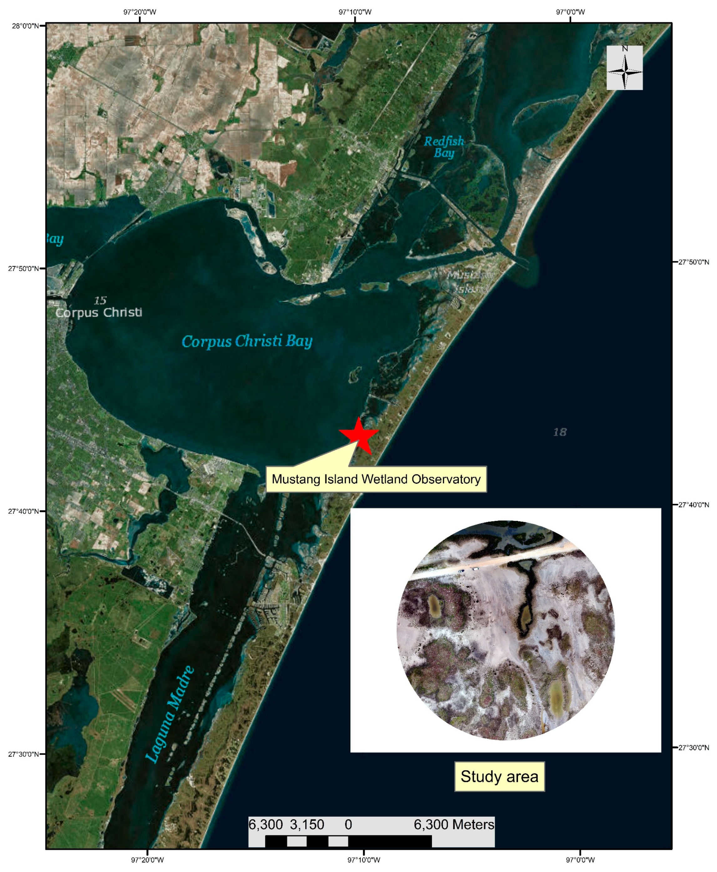
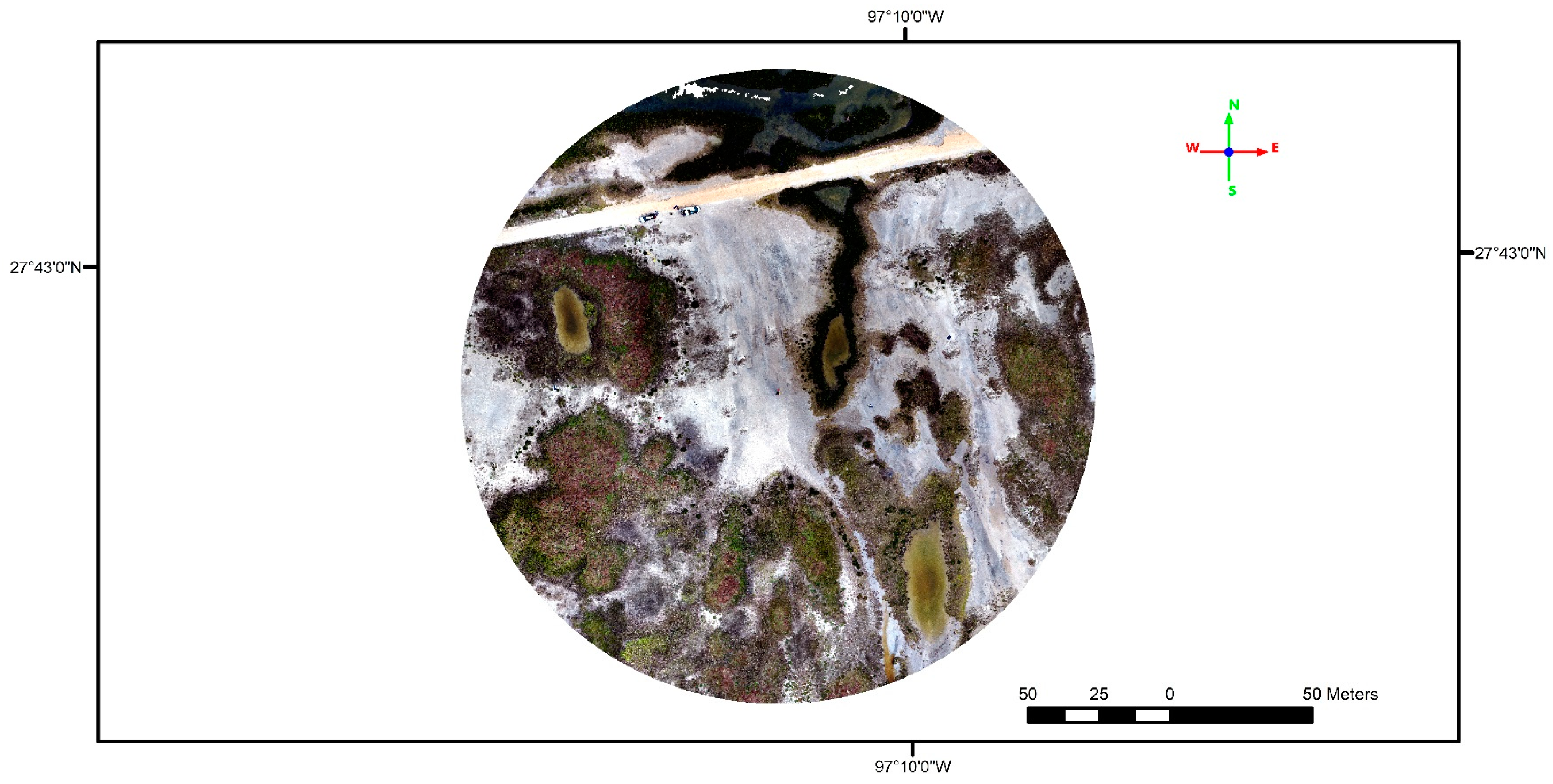
2.1. Study Site
2.2. Dataset
2.2.1. TLS
2.2.2. UAS-SfM
- Image sequences are input into the software and a keypoint detection algorithm, such as the scale invariant feature transform (SIFT), is used to automatically extract features and find keypoint correspondences between overlapping images using a keypoint descriptor. SIFT is a well-known computer vision algorithm that allows for feature detection regardless of scale, camera rotations, camera perspectives, and changes in illumination [31].
- A least squares bundle block adjustment is performed to minimize the errors in the correspondences by simultaneously solving for camera interior and exterior orientation. Based on this reconstruction, the matching points are verified and their 3D coordinates calculated to generate a sparse point cloud. Without any additional information, the coordinate system is arbitrary in translation and rotation and has inaccurate scale.
- To further constrain the problem and develop a georectified point cloud, ground control points (GCPs) and/or initial camera positions (e.g., from onboard GNSS) are introduced to constrain the solution. The input GCPs can be used to transform the point coordinates to a real-world coordinate system and to optimize rectification.
- Finally, the interior and exterior orientation for each image are used as input into a MultiView Stereo (MVS) algorithm, which attempts to densify the point cloud by projecting every image pixel, or at a reduced scale. This so called “dense matching” phase can be highly impacted by variations in surface texture as well as the MVS algorithm utilized.
3. Method
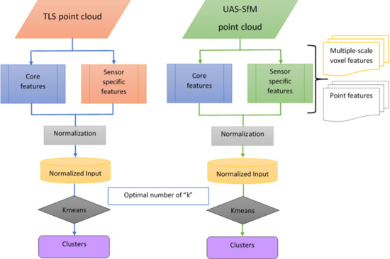
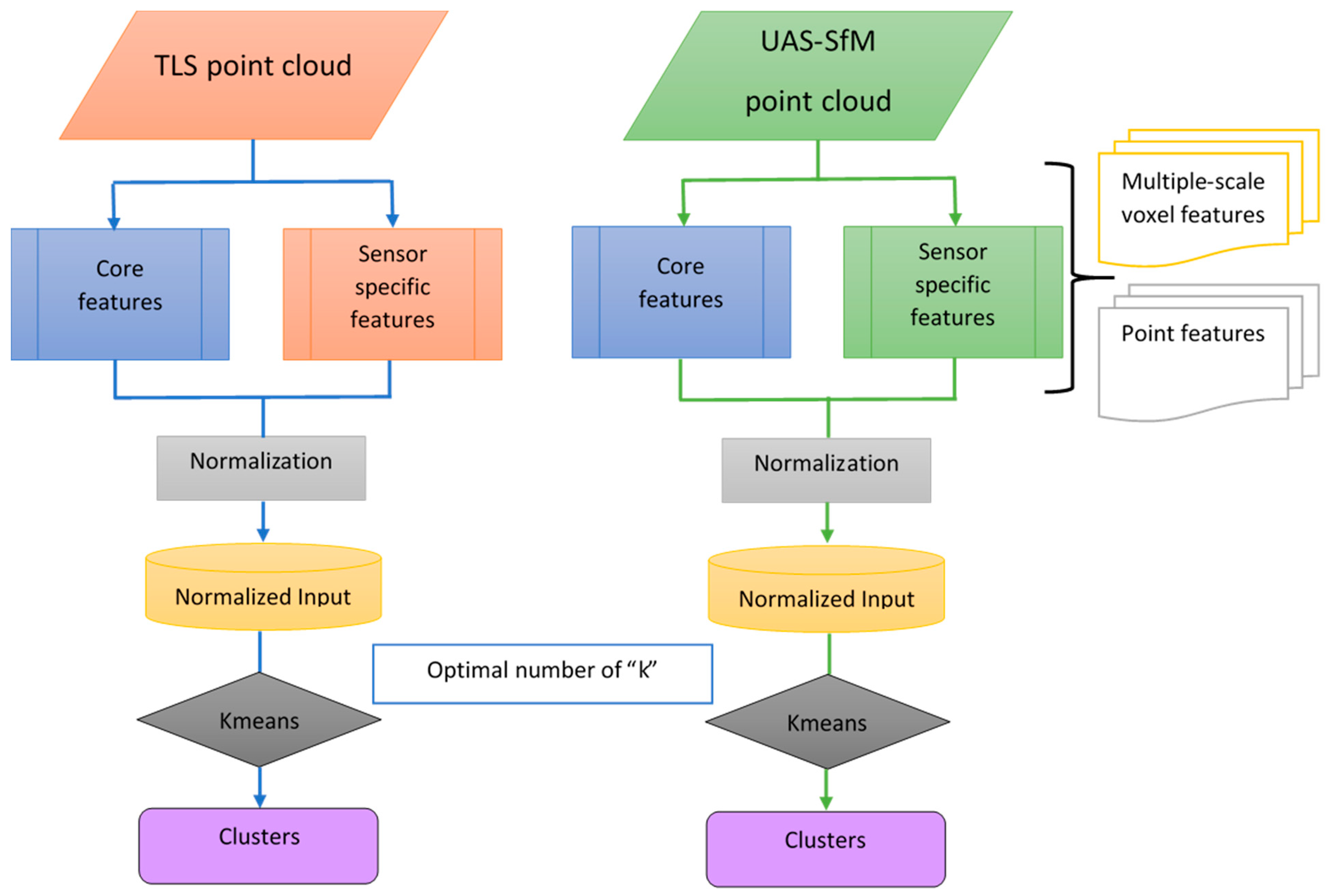
3.1. Overview
3.2. Feature Engineering
- TLS point features are height “z” (elevation), relative reflectance, and waveform deviation. Information about these features are described in [23].
- UAS-SfM point features are height “z” (elevation), Red (R), Green (G) and Blue (B) reflectance values. The R, G, and B pixel brightness values are based on the measurement of reflected radiation from different features on the ground. These values will depend on how the SfM software texturizes the point cloud data using the overlapping pixel values from the onboard digital camera. Although these values are not calibrated reflectance values, spectral response patterns of the land cover across the visual spectrum is captured in the data and this information is expected to be useful for aiding SfM point cloud segmentation of the land cover.
- The large-scale voxel statistical measures help identify the general environment of the voxel. Coarser scale voxels of size 697 × 697 × 7.6 cm were selected to capture broader spatial scale differences between environment types, such as the general location of a voxel within a tidal flat or a generally vegetated area. Tidal flats typically span several meters.
- The finer scale voxels provide information as to finer scale differences that would be averaged out by larger voxels such as differences between types of foliage. The finer scale voxel for this data set, 170 × 170 × 1.9 cm, was selected to match the variability of such parts of the scene and provide the information to the algorithm to potentially differentiate these voxels. For example, salt marsh plants such as Batis maritima at the study site are dioecious, perennial sub shrubs with heights in the range of 0.1–1.5 m and a span of 1–2 m for a group of plants [23]. Furthermore, portions of tidal flats will have points concentrated over a thin slice. Additionally, selecting a smaller size for the finer scale voxel would have resulted in less than the required minimum of 10 points imposed for statistical feature extraction for a relatively large number of voxels.
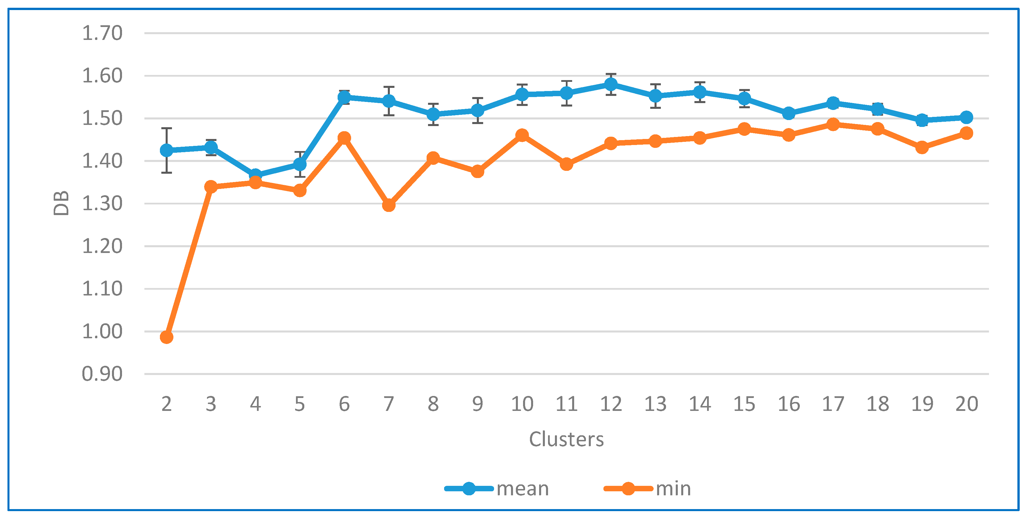
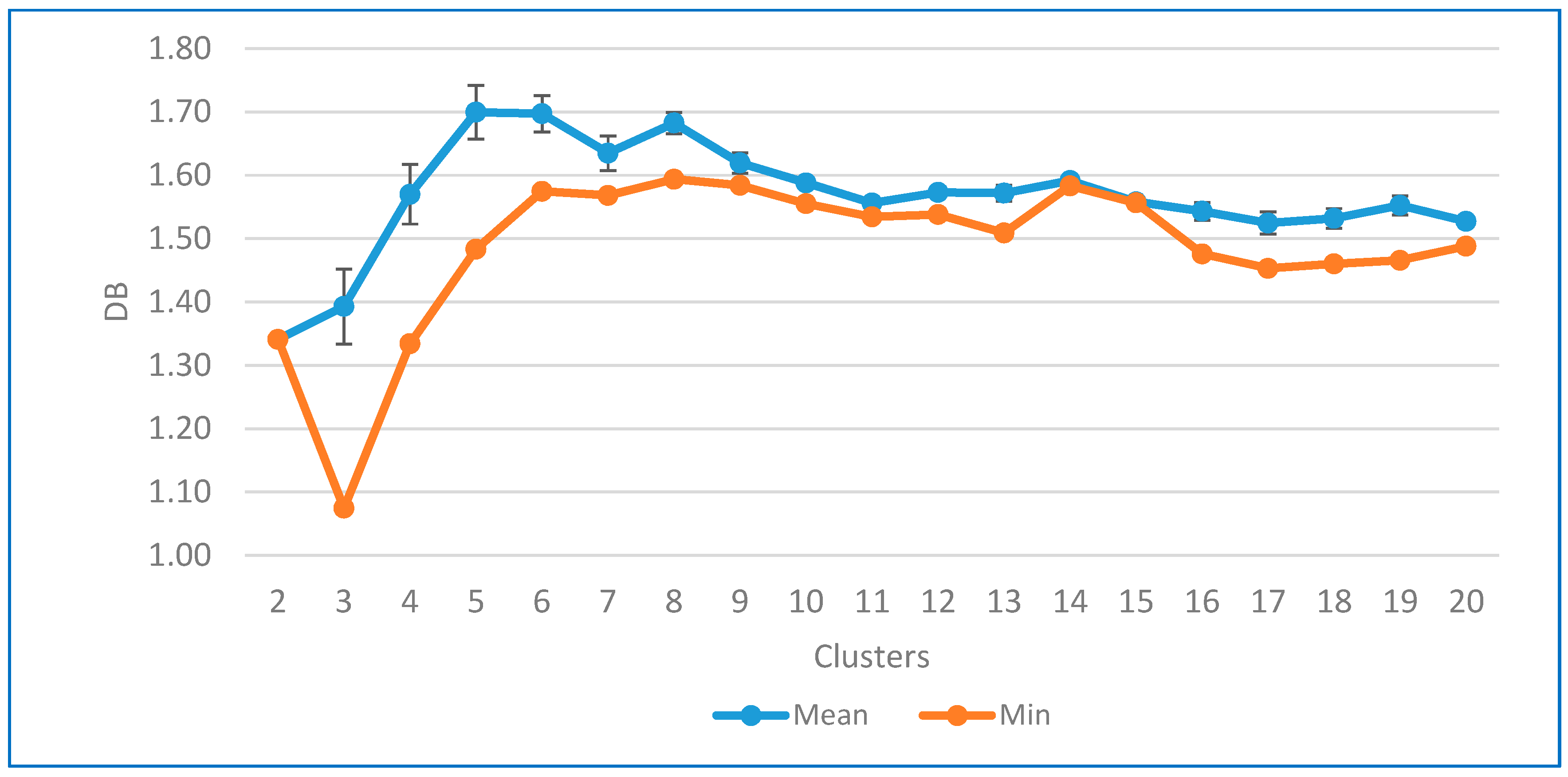
3.3. Determination of the Number of Clusters
4. Results and Discussion
4.1. Selection of the Number of Clusters
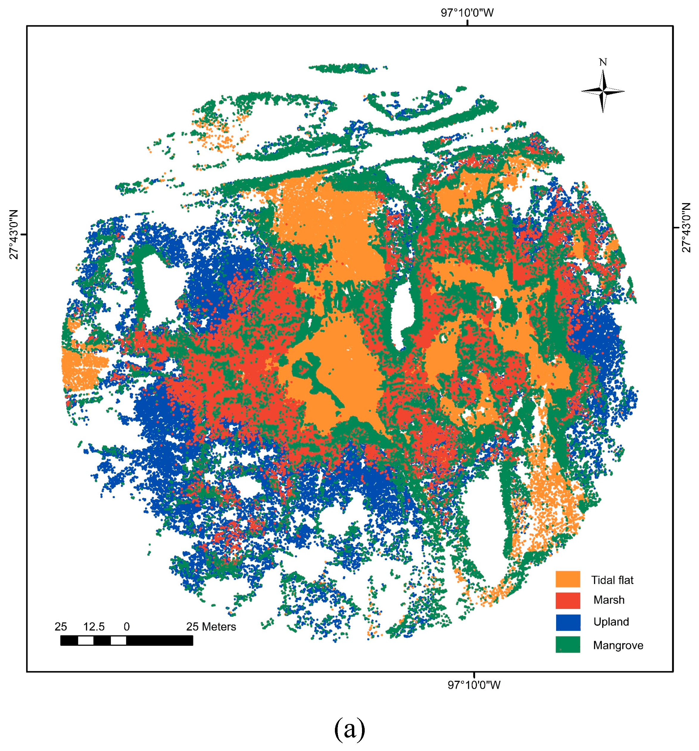
4.2. Comparative Description of the TLS and UAS-SfM Clusters
- With the advantage of a nadir view, UAS-SfM provides a point cloud of better coverage for this study area, while TLS is limited by the slant scan angle and suffers from vegetation occlusion which results in a less coverage point cloud.
- With RGB camera and photogrammetry technique, the UAS-SfM point cloud can capture the submerged flats in shallow water where the water is clear enough to reconstruct features on the bottom. With TLS using a NIR laser pulse, the pulse is likely bouncing away or sometimes absorbed at the area covered by water. As a result, the TLS provides few points at the submerged flats.
- Avicennia germinans (black mangrove) (green) are dominated and represented as cluster 6 in TLS and cluster 1 in UAS-SfM. The two-point clouds lead to very similar results, 12.1% of the scene for TLS and 11% for UAS. The high vegetation areas are easily identifiable for both methods as they stand out from a top down view (UAS-SfM) or a slant angle view (TLS).
- Upland vegetation (blue) are mainly populated by Zchizachyrium littorale (coastal bluestem) and Spartina patens (gulf cordgrass). They are represented as cluster 5 in TLS and cluster 2 in UAS. 28.8% of the UAS-SfM point cloud versus only 21.4% of the TLS point cloud are identified as the upland vegetation. These vegetated areas are located away from all three TLS scan positions and occlusions occur more frequently away from the scanner. Without the occlusion effect, UAS-SfM captures a larger fraction of these vegetation areas than TLS.
- Batis maritima (pickle weed), Monanthochloe litoralis (shoregrass), and Salicornia spp. (glasswort) are plants commonly found in the low and high marsh environments at the study site. For the UAS-SfM data set, the marsh vegetation areas (red) are the result of the combination of clusters 5 and 7. In the TLS point cloud, these areas are represented in a single cluster, cluster 1. A higher portion, 35%, of the TLS point cloud was identified as marsh vegetation points as compared to 33.2% for the UAS-SfM data. The higher percentage is likely due to the fact that these vegetated areas are closer to all three TLS scan positions and have an advantage of higher density point clouds.
4.3. Clustering Accurancy Assessment
4.4. Feature Importance
5. Conclusions
Author Contributions
Acknowledgments
Conflicts of Interest
References
- Cahoon, D.R.; Hensel, P.F.; Spencer, T.; Reed, D.J.; McKee, K.L.; Saintilan, N. Coastal wetland vulnerability to relative sea-level rise: Wetland elevation trends and process controls. In Wetlands and Natural Resource Management; Springer: Berlin/Heidelberg, Germany, 2006; pp. 271–292. [Google Scholar]
- Ford, M.A.; Cahoon, D.R.; Lynch, J.C. Restoring marsh elevation in a rapidly subsiding salt marsh by thin-layer deposition of dredged material. Ecol. Eng. 1999, 12, 189–205. [Google Scholar] [CrossRef]
- Schmid, K.A.; Hadley, B.C.; Wijekoon, N. Vertical accuracy and use of topographic LIDAR data in coastal marshes. J. Coast. Res. 2011, 27, 116–132. [Google Scholar] [CrossRef]
- Wang, C.; Menenti, M.; Stoll, M.P.; Feola, A.; Belluco, E.; Marani, M. Separation of Ground and Low Vegetation Signatures in LiDAR Measurements of Salt-Marsh Environments. IEEE Trans. Geosci. Remote Sens. 2009, 47, 2014–2023. [Google Scholar] [CrossRef]
- Rosso, P.H.; Ustin, S.L.; Hastings, A. Use of lidar to study changes associated with Spartina invasion in San Francisco Bay marshes. Remote Sens. Environ. 2006, 100, 295–306. [Google Scholar] [CrossRef]
- Sturdivant, E.J.; Lentz, E.E.; Thieler, E.R.; Farris, A.S.; Weber, K.M.; Remsen, D.P.; Miner, S.; Henderson, R.E. UAS-SfM for coastal research: Geomorphic feature extraction and land cover classification from high-resolution elevation and optical imagery. Remote Sens. 2017, 9, 1020. [Google Scholar] [CrossRef]
- Lemmens, M. Terrestrial Laser Scanning. In Geo-Information: Technologies, Applications and the Environment; Springer: Dordrecht, The Netherlands, 2011; pp. 101–121. [Google Scholar]
- Starek, M.J.; Mitasova, H.; Hardin, E.; Weaver, K.; Overton, M.; Harmon, R.S. Modeling and analysis of landscape evolution using airborne, terrestrial, and laboratory laser scanning. Geosphere 2011, 7, 1340–1356. [Google Scholar] [CrossRef]
- Starek, M.J.; Mitásová, H.; Wegmann, K.; Lyons, N. Space-time cube representation of stream bank evolution mapped by terrestrial laser scanning. IEEE Geosci. Remote Sens. Lett. 2013, 10, 1369–1373. [Google Scholar] [CrossRef]
- Fan, L.; Powrie, W.; Smethurst, J.; Atkinson, P.M.; Einstein, H. The effect of short ground vegetation on terrestrial laser scans at a local scale. ISPRS J. Photogramm. Remote Sens. 2014, 95, 42–52. [Google Scholar] [CrossRef]
- Fan, L.; Atkinson, P.M. Accuracy of digital elevation models derived from terrestrial laser scanning data. IEEE Geosci. Remote Sens. Lett. 2015, 12, 1923–1927. [Google Scholar] [CrossRef]
- Friess, D.A.; Moller, I.; Spencer, T.; Smith, G.M.; Thomson, A.G.; Hill, R.A. Coastal saltmarsh managed realignment drives rapid breach inlet and external creek evolution, Freiston Shore (UK). Geomorphology 2014, 208, 22–33. [Google Scholar] [CrossRef]
- Xie, W.M.; He, Q.; Zhang, K.Q.; Guo, L.C.; Wang, X.Y.; Shen, J.; Cui, Z. Application of terrestrial laser scanner on tidal flat morphology at a typhoon event timescale. Geomorphology 2017, 292, 47–58. [Google Scholar] [CrossRef]
- Olagoke, A.; Proisy, C.; Feret, J.B.; Blanchard, E.; Fromard, F.; Mehlig, U.; de Menezes, M.M.; dos Santos, V.F.; Berger, U. Extended biomass allometric equations for large mangrove trees from terrestrial LiDAR data. Trees Struct Funct 2016, 30, 935–947. [Google Scholar] [CrossRef]
- Klemas, V.V. Coastal and environmental remote sensing from unmanned aerial vehicles: An overview. J. Coast. Res. 2015, 31, 1260–1267. [Google Scholar] [CrossRef]
- Ramírez-Juidías, E. Study of erosion processes in the Tinto salt-marshes with remote sensing images. Adv. Image Video Process. 2014, 2, 39–52. [Google Scholar] [CrossRef]
- Kalacska, M.; Chmura, G.L.; Lucanus, O.; Berube, D.; Arroyo-Mora, J.P. Structure from motion will revolutionize analyses of tidal wetland landscapes. Remote Sens. Environ. 2017, 199, 14–24. [Google Scholar] [CrossRef]
- Westoby, M.J.; Brasington, J.; Glasser, N.F.; Hambrey, M.J.; Reynolds, J.M. ‘Structure-from-Motion’ photogrammetry: A low-cost, effective tool for geoscience applications. Geomorphology 2012, 179, 300–314. [Google Scholar] [CrossRef]
- Starek, M.J.; Davis, T.; Prouty, D.; Berryhill, J. Small-scale UAS for geoinformatics applications on an island campus. In Proceedings of the 2014 Ubiquitous Positioning Indoor Navigation and Location Based Service (UPINLBS), Corpus Christ, TX, USA, 20–21 November 2014; pp. 120–127. [Google Scholar]
- Slocum, R.K.; Parrish, C.E. Simulated imagery rendering workflow for uas-based photogrammetric 3d reconstruction accuracy assessments. Remote Sens. 2017, 9, 396. [Google Scholar] [CrossRef]
- Starek, M.J.; Giessel, J. Fusion of UAS-based structure-from-motion and optical inversion for seamless topo-bathymetric mapping. In Proceedings of the 2017 IEEE International Geoscience and Remote Sensing Symposium (IGARSS), Fort Worth, TX, USA, 23–28 July 2017; pp. 2999–3002. [Google Scholar]
- Chu, T.X.; Chen, R.Z.; Landivar, J.A.; Maeda, M.M.; Yang, C.H.; Starek, M.J. Cotton growth modeling and assessment using unmanned aircraft system visual-band imagery. J. Appl. Remote Sens. 2016, 10, 036018. [Google Scholar] [CrossRef]
- Nguyen, C.; Starek, M.J.; Tissot, P.; Gibeaut, J. Unsupervised clustering method for complexity reduction of terrestrial lidar data in marshes. Remote Sens. 2018, 10, 133. [Google Scholar] [CrossRef]
- Paine, J.G.; White, W.A.; Smyth, R.C.; Andrews, J.R.; Gibeaut, J.C. Mapping coastal environments with lidar and EM on Mustang Island, Texas, U.S. Lead. Edge 2004, 23, 894–898. [Google Scholar] [CrossRef]
- Church, J.A.; White, N.J. A 20th century acceleration in global sea-level rise. Geophys. Res. Lett. 2006, 33, 1944–8007. [Google Scholar] [CrossRef]
- Wang, G.; Soler, T. Measuring land subsidence using GPS: Ellipsoid height versus orthometric height. J. Surv. Eng. 2014, 141, 05014004. [Google Scholar] [CrossRef]
- Raber, G.T.; Jensen, J.R.; Hodgson, M.E.; Tullis, J.A.; Davis, B.A.; Berglund, J. Impact of lidar nominal post-spacing on DEM accuracy and flood zone delineation. Photogramm. Eng. Remote Sens. 2007, 73, 793–804. [Google Scholar] [CrossRef]
- Perroy, R.L.; Bookhagen, B.; Asner, G.P.; Chadwick, O.A. Comparison of gully erosion estimates using airborne and ground-based LiDAR on Santa Cruz Island, California. Geomorphology 2010, 118, 288–300. [Google Scholar] [CrossRef]
- Douillard, B.; Underwood, J.; Kuntz, N.; Vlaskine, V.; Quadros, A.; Morton, P.; Frenkel, A. On the segmentation of 3D LIDAR point clouds. In Proceedings of the 2011 IEEE International Conference on Robotics and Automation (ICRA), Shanghai, China, 9–13 May 2011; pp. 2798–2805. [Google Scholar]
- Strecha, C.; Küng, O.; Fua, P. Automatic mapping from ultra-light UAV imagery. In Proceedings of the EuroCOW 2012, Barceloa, Spain, 8–10 February 2012. [Google Scholar]
- Lowe, D.G. Distinctive image features from scale-invariant keypoints. Int. J. Comput. Vis. 2004, 60, 91–110. [Google Scholar] [CrossRef]
- Schwind, M.; Starek, M. How to produce high-quality 3D point clouds Structure-from-Motion Photogrammetry. Gim Int. Worldw. Mag. Geomat. 2017, 31, 36–39. [Google Scholar]
- Jain, A.K. Data clustering: 50 years beyond K-means. Pattern Recognit. Lett. 2010, 31, 651–666. [Google Scholar] [CrossRef]
- Wakita, T.; Susaki, J. Multi-scale based extracion of vegetation from terrestrial lidar data for assessing local landscape. Int. Arch. Photogramm. 2015, II-3/W4, 263–270. [Google Scholar] [CrossRef]
- Vandapel, N.; Huber, D.F.; Kapuria, A.; Hebert, M. Natural terrain classification using 3-d ladar data. In Proceedings of the 2004 IEEE International Conference on Robotics and Automation, New Orleans, LA, USA, 26 April–1 May 2004; pp. 5117–5122. [Google Scholar]
- Carlberg, M.; Gao, P.; Chen, G.; Zakhor, A. Classifying urban landscape in aerial LiDAR using 3D shape analysis. In Proceedings of the 2009 16th IEEE International Conference on Image Processing (ICIP), Cairo, Egypt, 7–10 November 2009; pp. 1701–1704. [Google Scholar]
- Visalakshi, N.K.; Thangavel, K. Impact of normalization in distributed k-means clustering. Int. J. Soft Comput. 2009, 4, 168–172. [Google Scholar]
- Bowen, Z.H.; Waltermire, R.G. Evaluation of light detection and ranging (lidar) for measuring river corridor topography 1. JAWRA J. Am. Water Resour. Assoc. 2002, 38, 33–41. [Google Scholar] [CrossRef]
- Davies, D.L.; Bouldin, D.W. A cluster separation measure. IEEE Trans. Pattern Anal. Mach. Intell. 1979, 224–227. [Google Scholar] [CrossRef]
- Lloyd, S.P. Least-Squares Quantization in Pcm. IEEE Trans. Inf. Theory 1982, 28, 129–137. [Google Scholar] [CrossRef]
- Milan, D.J.; Heritage, G.L.; Hetherington, D. Application of a 3D laser scanner in the assessment of erosion and deposition volumes and channel change in a proglacial river. Earth Surf. Process. Landf. 2007, 32, 1657–1674. [Google Scholar] [CrossRef]
- Montgomery, D.C.; Runger, G.C.; Hubele, N.F. Engineering Statistics; John Wiley & Sons: Hoboken, NJ, USA, 2009. [Google Scholar]


| Pulse repetition rate | Up to 300,000 kHz |
| Laser wavelength | 1550 nm |
| Beam divergence | 0.3 mrad |
| Spot size | 3 cm at 100 m distance |
| Range | 1.5 m (min), 600 m (max) * |
| Field of view | 100° vertical x 360° horizontal |
| Repeatability | 3 mm (1 sigma @ 100 m range) |
| Minimum stepping angle | 0.0024° |
| Tidal Flat (orange) | Mangrove (green) | Upland Vegetation (blue) | Marsh Vegetation (red) | Noise (gray) | |
|---|---|---|---|---|---|
| Clusters | 3, 4 | 6 | 5 | 1 | 2, 7 |
| Number of points | 8,452,659 | 3,242,034 | 5,738,119 | 9,370,571 | 13,270 |
| Percentage of points | 31.52% | 12.09% | 21.40% | 34.94% | 0.05% |
| Tidal Flat (orange) | Mangrove (green) | Upland Vegetation (blue) | Marsh Vegetation (red) | Noise (gray) | |
|---|---|---|---|---|---|
| Clusters | 3, 4 | 1 | 2 | 5,7 | 6 |
| Number of points | 10,459,173 | 4,231,130 | 11,128,581 | 12,858,377 | 13,280 |
| Percentage of points | 27.03% | 10.94% | 28.76% | 33.23% | 0.03% |
| TLS | Ground Truth (Points) | User’s Accuracy | |||
|---|---|---|---|---|---|
| Tidal Flat | Vegetated Areas | Total | |||
| Classification by Clusters (points) | Tidal flat | 4,359,251 | 34,543 | 4,393,794 | 99.2% |
| Vegetated areas | 650,614 | 7,283,037 | 7,933,651 | 91.8% | |
| Total | 5,009,865 | 7,317,580 | 12,327,445 | ||
| Producer’s Accuracy | 87.0% | 99.5% | Total: 93.3% | ||
| UAS-SfM | Ground Truth (Points) | User’s Accuracy | |||
|---|---|---|---|---|---|
| Tidal Flat | Vegetated Areas | Total | |||
| Classification by Clusters (points) | Tidal flat | 4,046,110 | 302,566 | 4,348,676 | 93.0% |
| Vegetated areas | 225,203 | 15,664,999 | 15,890,202 | 98.6% | |
| Total | 4,271,313 | 15,967,565 | 20,238,878 | ||
| Producer’s Accuracy | 94.7% | 98.1% | Total: 96.4% | ||
| Number of Clusters | Producer’s Accuracy | User’s Accuracy | ||
|---|---|---|---|---|
| Tidal Flat | Vegetated Areas | Tidal Flat | Vegetated Areas | |
| 5 | 93.4% | 98.8% | 98.1% | 95.6% |
| 6 | 87.0% | 99.5% | 99.2% | 91.8% |
| 7 | 87.0% | 99.5% | 99% | 91.8% |
| 8 | 87.6% | 99.8% | 99.7% | 92.2% |
| Number of Clusters | Producer’s Accuracy | User’s Accuracy | ||
|---|---|---|---|---|
| Tidal Flat | Vegetated Areas | Tidal Flat | Vegetated Areas | |
| 5 | 99.3% | 87.7% | 68.3% | 99.8% |
| 6 | 87.5% | 86.6% | 63.6% | 96.3% |
| 7 | 94.7% | 98.1% | 93.0% | 98.6% |
| 8 | 87.5% | 98.0% | 92.3% | 96.7% |
| Number of Clusters | Producer’s Accuracy | User’s Accuracy | ||
|---|---|---|---|---|
| Exposed Ground | Vegetated Areas | Exposed Ground | Vegetated Areas | |
| 5 | 99.99% | 99.74% | 99.12% | 100.00% |
| 6 | 99.98% | 99.95% | 99.82% | 100.00% |
| 7 | 99.99% | 99.95% | 99.82% | 100.00% |
| 8 | 99.72% | 99.97% | 99.91% | 99.92% |
| Number of Clusters | Producer’s Accuracy | User’s Accuracy | ||
|---|---|---|---|---|
| Exposed Ground | Vegetated Areas | Exposed Ground | Vegetated Areas | |
| 5 | 98.89% | 99.82% | 98.51% | 99.87% |
| 6 | 99.58% | 95.90% | 74.51% | 99.95% |
| 7 | 99.01% | 99.04% | 92.54% | 99.80% |
| 8 | 98.26% | 99.05% | 92.49% | 99.79% |
| TLS | UAS-SfM | ||
|---|---|---|---|
| Features | F Statistic | Features | F Statistic |
| Curvature 2 of small voxel | 13,071,500 | σB of large voxel | 7,159,650 |
| Curvature 2 of large voxel | 12,032,700 | σG of large voxel | 6,839,710 |
| σD of large voxel | 9,260,570 | σB of small voxel | 6,086,370 |
| σD of small voxel | 7,855,800 | σG of small voxel | 6,084,770 |
| σR of large voxel | 7,274,380 | σR of large voxel | 5,793,100 |
| σR of small voxel | 6,361,320 | σR of small voxel | 5,715,920 |
| Elevation (Z) | 5,485,250 | Blue (B) | 5,290,480 |
| Waveform Deviation (D) | 5,449,800 | Green (G) | 5,149,100 |
| σZ of large voxel | 5,110,470 | Curvature 2 of small voxel | 4,878,490 |
| Reflectance (R) | 3,461,560 | Red (R) | 4,758,860 |
| σZ of small voxel | 3,062,030 | Curvature 2 of large voxel | 3,681,740 |
| Curvature 1 of small voxel | 1,428,290 | Elevation (Z) | 2,590,360 |
| Curvature 1 of large voxel | 1,422,150 | σZ of small voxel | 2,123,120 |
| σZ of large voxel | 1,678,420 | ||
| Curvature 1 of large voxel | 1,363,320 | ||
| Curvature 1 of small voxel | 1,152,010 | ||
© 2019 by the authors. Licensee MDPI, Basel, Switzerland. This article is an open access article distributed under the terms and conditions of the Creative Commons Attribution (CC BY) license (http://creativecommons.org/licenses/by/4.0/).
Share and Cite
Nguyen, C.; Starek, M.J.; Tissot, P.; Gibeaut, J. Unsupervised Clustering of Multi-Perspective 3D Point Cloud Data in Marshes: A Case Study. Remote Sens. 2019, 11, 2715. https://doi.org/10.3390/rs11222715
Nguyen C, Starek MJ, Tissot P, Gibeaut J. Unsupervised Clustering of Multi-Perspective 3D Point Cloud Data in Marshes: A Case Study. Remote Sensing. 2019; 11(22):2715. https://doi.org/10.3390/rs11222715
Chicago/Turabian StyleNguyen, Chuyen, Michael J. Starek, Philippe Tissot, and James Gibeaut. 2019. "Unsupervised Clustering of Multi-Perspective 3D Point Cloud Data in Marshes: A Case Study" Remote Sensing 11, no. 22: 2715. https://doi.org/10.3390/rs11222715
APA StyleNguyen, C., Starek, M. J., Tissot, P., & Gibeaut, J. (2019). Unsupervised Clustering of Multi-Perspective 3D Point Cloud Data in Marshes: A Case Study. Remote Sensing, 11(22), 2715. https://doi.org/10.3390/rs11222715