Letter

The Radiative Transfer Characteristics of the O2 Infrared Atmospheric Band in Limb-Viewing Geometry

1
City College, Wuhan University of Science and Technology, Wuhan 430083, China
2
State Key Laboratory of Magnetic Resonance and Atomic and Molecular Physics, Wuhan Institute of Physics and Mathematics, Chinese Academy of Sciences, Wuhan National Laboratory for Optoelectronics, Wuhan 430071, China
3
Key Laboratory of Spectral Imaging Technology of Chinese Academy of Sciences, Xi’an Institute of Optics and Precision Mechanics, Chinese Academy of Sciences, Xi’an 710119, China
*
Author to whom correspondence should be addressed.
Remote Sens. 2019, 11(22), 2702; https://doi.org/10.3390/rs11222702
Submission received: 29 September 2019 / Revised: 13 November 2019 / Accepted: 15 November 2019 / Published: 18 November 2019

Abstract

:
The O2(a1Δg) emission near 1.27 μm provides an important means to remotely sense the thermal characteristics, dynamical features, and compositional structures of the upper atmosphere because of its photochemistry and spectroscopic properties. In this work, an emission–absorption transfer model for limb measurements was developed to calculate the radiation and scattering spectral brightness by means of a line-by-line approach. The nonlocal thermal equilibrium (non-LTE) model was taken into account for accurate calculation of the O2(a1Δg) emission by incorporating the latest rate constants and spectral parameters. The spherical adding and doubling methods were used in the multiple scattering model. Representative emission and absorption line shapes of the O 2 ( a 1 Δ g , υ = 0 ) O 2 ( X Σ g 3 , υ = 0 ) band and their spectral behavior varying with altitude were examined. The effects of solar zenith angle, surface albedo, and aerosol loading on the line shapes were also studied. This paper emphasizes the advantage of using infrared atmospheric band for remote sensing of the atmosphere from 20 up to 120 km, a significant region where the strongest coupling between the lower and upper atmosphere occurs.

Graphical Abstract

1. Introduction

Measurements of radiation of electronically excited molecular oxygen in the atmospheric band O2 ( b Σ g 1 , υ = 0 X Σ g 3 , υ = 0 ) at 762 nm and in the infrared atmospheric band O2 ( a Δ g 1 , υ = 0 X Σ g 3 , υ = 0 ) at 1.27 µm provide fundamental probes into energy transfer, compositional structures, and thermodynamic and dynamic features of the upper stratosphere, mesosphere, and lower thermosphere. Compared with the atmospheric band, the infrared atmospheric band has a greater advantage in bright signal (the strongest radiative signal in the visible and near-infrared region of the spectrum) and extended altitude (from 20 to 120 km). Therefore, the O2(a1Δg) airglow is selected as the target source by many space-based instruments aboard rockets and satellites. Mesosphere-Thermosphere Emissions for Ozone Remote Sensing (METEORS) [1], Optical Spectrograph and Infrared Imager System (OSIRIS) [2], and Sounding of the Atmosphere using Broadband Emission Radiometry (SABER) [3] prove that the O3 altitude distribution can be extracted by incorporating O2(a1Δg) dayglow observations. The remarkable success of Spectroscopy for the Investigation of the Characteristics of the Atmosphere of Mars (SPICAM) instrument onboard the Mars Express orbiter has stimulated interest in taking measurements of O2(a1Δg) dayglow emission and their comparison with photochemical models to yield the Martian water cycle [4]. The Mesospheric Imaging Michelson Interferometer (MIMI) supported by Canada’s StaSci program and the Waves Michelson Interferometer (WAMI) funded by NASA’s MIDEX program use a Michelson interferometer to observe the strong and weak groups of emission lines in the O2 infrared atmospheric band to achieve simultaneous measurements of the Earth temperature and wind [5]. More recently, the the Near-space Wind and Temperature Sensing Interferometer (NWTSI) instrument, which closely follows the WAMI and MIMI concepts, was designed ingeniously to improve the accuracies of wind and temperature measurements in the near space [6]. Last year, Wu et al. reported the application of O2(a1Δg) dayglow for wind observation with a Doppler Asymmetric Spatial Heterodyne (DASH) type instrument from a limb-viewing satellite by measuring Doppler shifts of the emission line O19P18, which were detectable due to their weak self-absorption, bright radiation intensity, and large spectral separation range [7].
High-resolution spectra of the reflected and scattered sunlight near the O2 infrared atmospheric band also play a key role in atmospheric remote sensing, especially for the determination of CO2 mixing ratio columns from space. Several infrared CO2 absorption bands (e.g., 15, 4.3, 2.7, 2.0, and 1.6 µm) can be used for CO2 mixing ratio retrievals by the use of atmospheric pressure and temperature, which can be retrieved from the O2 absorption bands (e.g., 0.76 or 1.27 µm) [8]. The O2 absorption band around 1.27 µm is much weaker than the 0.76 µm band, so the radiative transfer modeling will be more accurate. In addition, the 1.27 µm band is much closer in wavelength to the CO2 absorption bands (1.6 and 2.0 µm), which reduces uncertainties caused by spectral variations in the atmospheric path. Sun et al. evaluated the use of O2(a1g) band in spaceborne remote sensing of greenhouse gas with modern spaceborne spectrometers [9]. Dobler et al. discussed the feasibility of determining surface pressure by measuring atmospheric O2 near the 1.27 µm band for determination of CO2 mixing ratio columns with a laser absorption spectrometer [10].
Depending on the atmospheric region, the O2(a1g) band can be observed both in emission and absorption, with the latter dominating below about 30 km. The absorption and emission spectral features also interact with each other in atmospheric remote sensing. Sharp et al. reported the impact of ambient O2(a1Δg) on O2 column remote sensing with satellite-based laser using absorption lines in the 1.27 µm band [11]. Bertaux et al. evaluated the contribution of O2(a1Δg) airglow to the retrieval accuracy of CO2 mixing ratio columns in the MicroCarb optical concept [12]. Wu et al. analyzed the spectral interference of scattered sunlight on the O2(a1Δg) dayglow observations and evaluated wind precision with and without the effect of spectral interference [7].
In this paper, we report the radiative transfer characteristics of the O2 infrared atmospheric band in limb-viewing geometry. Section 2 describes the photochemical reaction mechanism of the O2 infrared atmospheric band, the O2(a1Δg, v’ = 0) emission rates, and the O2(a1Δg, v’ = 0, J) rotational distribution. Section 3 presents the results of the limb spectral radiance and the line shape simulations of the O2(a1Δg) emission spectrum and multiple scattering spectrum as well as the total spectral radiance. The effects of solar zenith angle (SZA), surface albedo, and aerosol loading on the line shapes are also discussed in this Section. A concluding summary in Section 4 completes this paper.

2. The O2 Infrared Atmospheric Band

Molecular oxygen absorbs radiation in its two lowest-lying electronic transitions: O 2 ( a Δ g 1 ) O 2 ( X Σ g 3 ) at 1.27 µm (the infrared atmospheric band) and O 2 ( b Σ g 1 ) O 2 ( X Σ g 3 ) with bands at 762, 688, and 629 nm, which are referred to as the A, B, and γ atmospheric bands. The absorption line strength and spectral distribution of the four bands are shown in Figure 1. The B ( b Σ g 1 , υ = 1 X Σ g 3 , υ = 0 ) and γ ( b Σ g 1 , υ = 1 X Σ g 3 , υ = 0 ) bands do not produce airglow because the excited vibrational states are quenched into the v’ = 0 state before the electronic transition takes place. Compared with the A atmospheric band, the infrared atmospheric band provides a stronger radiative signal, covers a much more extended altitude region (between ~20 and 120 km in the dayglow), and suffers less from the self-absorption of O2 molecules in the ground state.

2.1. The O2(a1Δg) Photochemistry

The key to accurate calculation of the limb spectral radiance of the O2 infrared atmospheric band depends not only on an accurate knowledge of the atmospheric and spectroscopic parameters but also on a detailed accounting of all sources of O2(a1Δg) [14]. Remote sensing of airglow emissions has contributed significantly to the current understanding of the production and loss mechanisms of electronically excited O2(a1Δg). The metastable molecule O2(a1Δg) is formed in the processes of photodissociation of O3 and O2 by absorption of ultraviolet radiation of the sun. The first commonly accepted model of O3 and O2 photolysis was developed by Thomas (1984) [15] and Harris and Adams (1983) [16]. M.G. Mlynczak, S. Solomon, and D.S. Zaras significantly improved this model in 1993 (for the sake of brevity, this model is called MSZ) [14]. In 2011, Yankovsky et al. developed a complete model of electronic vibrational kinetics of O2 and O3 photolysis products (YM2011) [17,18]. In 2017, Martyshenko and Yankovsky solved the problem of systematic overestimation in the retrieve of ozone concentrations by taking the electronic vibrational kinetics of photolysis products of ozone and molecular oxygen O 2 ( b Σ g 1 , v ) and O 2 ( a Δ g 1 , v ) into the scheme of electronic vibrational kinetics of the products of O3 and O2 photolysis [19]. Figure 2 shows the dayglow production mechanism of the O2 infrared atmospheric band [20].
With the values of the rates of photodissociation and photoexcitation and the values of the rate constants of the processes considered by Yankovsky et al. [17,19], the O2(a1Δg) number density, n O 2 ( a Δ g 1 ) , can be calculated assuming photochemical equilibrium. Figure 3 shows the amounts of O2(a1Δg) attributable to each source of predominant mechanisms. The source corresponding to each curve is described and marked in the figure legend. It is apparent from this figure that the primary source for O2(a1Δg) is generated directly upon photolysis of O3. The coproduct O(1D) through energy transfer emerges as the secondary, parallel contribution and dominates the emission process above 100 km. The photoexcitation-induced O 2 ( b Σ g 1 ) becomes a major contributor between 65 and 85 km.

2.2. The O2(a1Δg, v’ = 0) Emission Rates

The excited vibrational states O 2 ( a Δ g 1 , ν 1 ) are quenched into the ground vibrational state O 2 ( a Δ g 1 , ν = 0 ) much more rapidly than the electronic transition. Figure 4 shows the modeled number densities of O2(a1Δg) molecules at ν = 0 , ν = 1 , and ν = 2 as a function of altitude. As can be seen, the contributions from the excited vibrational states O 2 ( a Δ g 1 , ν 1 ) are negligible, and vibrational distribution of the ground vibrational state O 2 ( a Δ g 1 , ν = 0 ) dominates the infrared atmospheric band:
n O 2 ( a Δ g 1 , ν = 0 ) n O 2 ( a Δ g 1 ) .
The local emission rate of the infrared atmospheric band O 2 ( a Δ g 1 , υ = 0 ) O 2 ( X Σ g 3 , υ = 0 ) , i.e., η 1.27 μ m , is obtained by multiplying its vibrational distribution n O 2 ( a Δ g 1 , ν = 0 ) and the Einstein transition probability A 1.27 μ m [3]:
η 1.27 μ m = A 1.27 μ m n O 2 ( a Δ g 1 , ν = 0 ) .
Figure 5 shows the calculated volume emission rate (VER) profiles of the O2 infrared atmospheric band under daytime condition in the four seasons in the Northern Hemisphere (simulated by taking the mid-latitude for example). As is apparent, there are only minor differences between different seasons. The VER for the summer illuminated atmosphere (July) is slightly larger at low altitude. The major reason for this behavior is the consequence of larger solar illumination at north latitude in summertime. The spring volume emission becomes the largest over the altitude region from 30 to 50 km because the ozone content is the most abundant in spring.

2.3. The O2(a1Δg, v’ = 0, J) Rotational Distribution

The spectral distribution of the O 2 ( a Δ g 1 , υ = 0 ) O 2 ( X Σ g 3 , υ = 0 ) vibrational transition band depends on the rotational distribution of the O 2 ( a Δ g 1 , υ = 0 ) state and their individual line shapes.
The emission rate per O 2 ( a Δ g 1 , υ = 0 ) molecule ε ( J , J ) of a given rotational transition J J is obtained by multiplying the particular Einstein coefficient for the vibration–rotation transition A J , J with the relative population of the upper level:
ε ( J , J ) = A J , J g J exp ( h c E v ( J ) / k T R ) Q t o t ( T )
where J and J are initial and final values of the total angular momentum of the transition, respectively; E v ( J ) is the upper state rotational term value; g J is the statistical weights of the initial level; k is the Boltzmann constant; h is the Planck constant; c is the speed of light; TR is the rotational temperature assumed to be in thermal equilibrium with the ambient atmospheric temperature; and Q t o t ( T ) is the electronic–rotational partition function given as [21]
Q t o t ( T ) = J g J exp ( h c E v ( J ) / k T R ) .
Figure 6a shows the emission spectrum as a function of the transition wavelength, which is displayed on the right scale. For comparison, the absorption line intensity from the HITRAN database [13] can also be found in this figure (left scale). As can be seen, the emission lines and the absorption ones show different distributions in spectrum. By simply doing a division, we could find the ratio of emission to absorption line strength for each line, which is shown in Figure 6b. This ratio is a temperature-dependent value, varying with the total angular momentum of the transition.

3. Limb Spectral Radiance

Figure 7 illustrates the construction of the path model in limb-viewing geometry. For the O2 infrared atmospheric band, a strong self-absorption appears because of the relatively large line strength of ground state. Therefore, the limb spectral radiance is not simply a straightforward Abel-type integration of the VER profile along the path between the emitter and the observer. The brightness is modified by the attenuation along the line-of-sight path. In addition, limb brightness measurements unavoidably include Rayleigh scattering and Mie scattering, which will be subject to the extinction process in the O2 infrared atmospheric band spectral region. For accurate calculation of the spectral brightness of the O2 infrared atmospheric band, the absorption for both emission lines and the scattered sunlight continuum background must be taken into consideration, especially at low tangent heights.

3.1. O2(a1Δg, v’ = 0) Emission Spectrum

As described above, O2(a1Δg, v’ = 0) distribution is in collisional and chemical balance. At lower altitude, the quenching-related decay of O2(a1Δg, v’ = 0) is significant because the probability of quenching determines the lifetime of O2(a1Δg, v’ = 0), while at higher altitude, the local thermodynamic equilibrium (LTE) is broken because of the presence of constant sources of excited molecular oxygen due to O2 and O3 photodissociation. O2(a1Δg) is formed mainly by photolysis of O3 in the Hartley band below about 100 km and by energy transfer from O(1D) above that altitude [20,22]. The collisional quenching of O2(b1Σg) with N2 and O2 also contributes to the production of O2(a1Δg), especially at 65–85 km. Thus, the distribution of O2(a1Δg, v’ = 0) is not strongly connected to the kinetic temperature and cannot be given by the Boltzmann distribution. This behavior is referred to as nonlocal thermal equilibrium (non-LTE).
In the non-LTE case, the source function of the O 2 ( a Δ g 1 , υ = 0 ) O 2 ( X Σ g 3 , υ = 0 ) transition is given by [23]
J ( ν ) B ( ν , T K ) exp ( h c k ( 1 T O 2 ( a Δ 1 g , ν = 0 ) 1 T K ) E O 2 ( a Δ g 1 , ν = 0 ) )
where B ( ν , T K ) is the value of the Planck function at wavenumber ν and temperature TK, E O 2 ( a Δ g 1 , ν = 0 ) = 7882.42   cm 1 is the vibrational energy of the O 2 ( a Δ g 1 , υ = 0 ) state, T O 2 ( a Δ g 1 , ν = 0 ) is the vibrational temperature and is expressed as
T O 2 ( a Δ g 1 , ν = 0 ) = E O 2 ( a Δ 1 g , ν = 0 ) k ln ( n O 2 ( X Σ g 3 , ν = 0 ) n O 2 ( a Δ 1 g , ν = 0 ) g O 2 ( a Δ 1 g , ν = 0 ) g O 2 ( X Σ g 3 , ν = 0 ) ) .
Here, g O 2 ( a Δ g 1 , ν = 0 ) and g O 2 ( X Σ g 3 , ν = 0 ) refer to the statistical weight of the O 2 ( a Δ g 1 ) and the O 2 ( b Σ g 1 ) states. It is important to note that the vibrational temperature, which, being substituted in Boltsmann distribution, gives the vibrational level population. Correspondingly, at the LTE conditions, the vibrational temperature becomes equal to a kinetic one.
When the self-absorption process is considered, the limb spectral brightness of any given rotational line in the O2 infrared atmospheric band can be carried out numerically by [23]
I E ( ν ) l = I E ( ν ) l 1 exp ( α ( ν ) l u l ) + J ( ν ) l α ( ν ) l n l z L z U τ ( ν , z , z U ) d z
where z is a certain position along the line of sight between the observation point z o b s and the point z s at the furthest extent of the limb; z U and z L are the upper and lower boundaries of layer l, respectively; α(ν) is the molecular absorption coefficient; n(z) is the number density of O2 molecules in the ground state; u l = n l ( z U z L ) is the layer absorber amount of layer l; and τ ( ν , z , z o b s ) is the atmospheric transmission caused by self-absorption effect between z and zobs, which can be given by
τ ( ν , z , z o b s ) = exp ( z s z o b s α ( ν , z ) n ( z ) d z ) .
It is obvious that the forward model for the spectral brightness has a strong dependence on the atmospheric temperature, which is concretely embodied in the self-absorption cross section, the line strength, and the Doppler width. In addition, the spectral brightness has a linear dependence on the VER profile. Figure 8 shows the calculated limb spectral brightness and the spectral radiance of the target layer at different tangent heights using the non-LTE model. As illustrated, the spectral radiance of the target layer comes closer to the limb spectral brightness at relatively high tangent heights (up to ~60 km), while at low altitude, the target layer radiance is relatively small compared with the limb brightness. Two factors explain this phenomenon: (1) O2 number density leads to a strong self-absorption at low altitude and (2) the lower the altitude, the smaller the O2(a1Δg) VER.
Figure 9 shows the spectral brightness and the atmospheric transmittance of a relatively strong line (R9Q10 at 1264.06 nm) of O2 infrared atmospheric band at the tangent height of 50 km. For comparison, the spectral line brightness neglecting self-absorption is also displayed in the same figure. As illustrated, the self-absorption of the R9Q10 line is significant even at 50 km tangent height. As a type of Doppler line shape, the value of the absorption cross section is large at the line center and decreases toward the two wings, so the process of self-absorption leads to a spectral line broadening for the emission line. Due to this broadening effect, the WAMI, MIMI, and NWTSI instruments cannot provide meaningful Doppler temperature, and the rotational temperatures need to be measured by observing relative radiation intensity of three rotational lines.
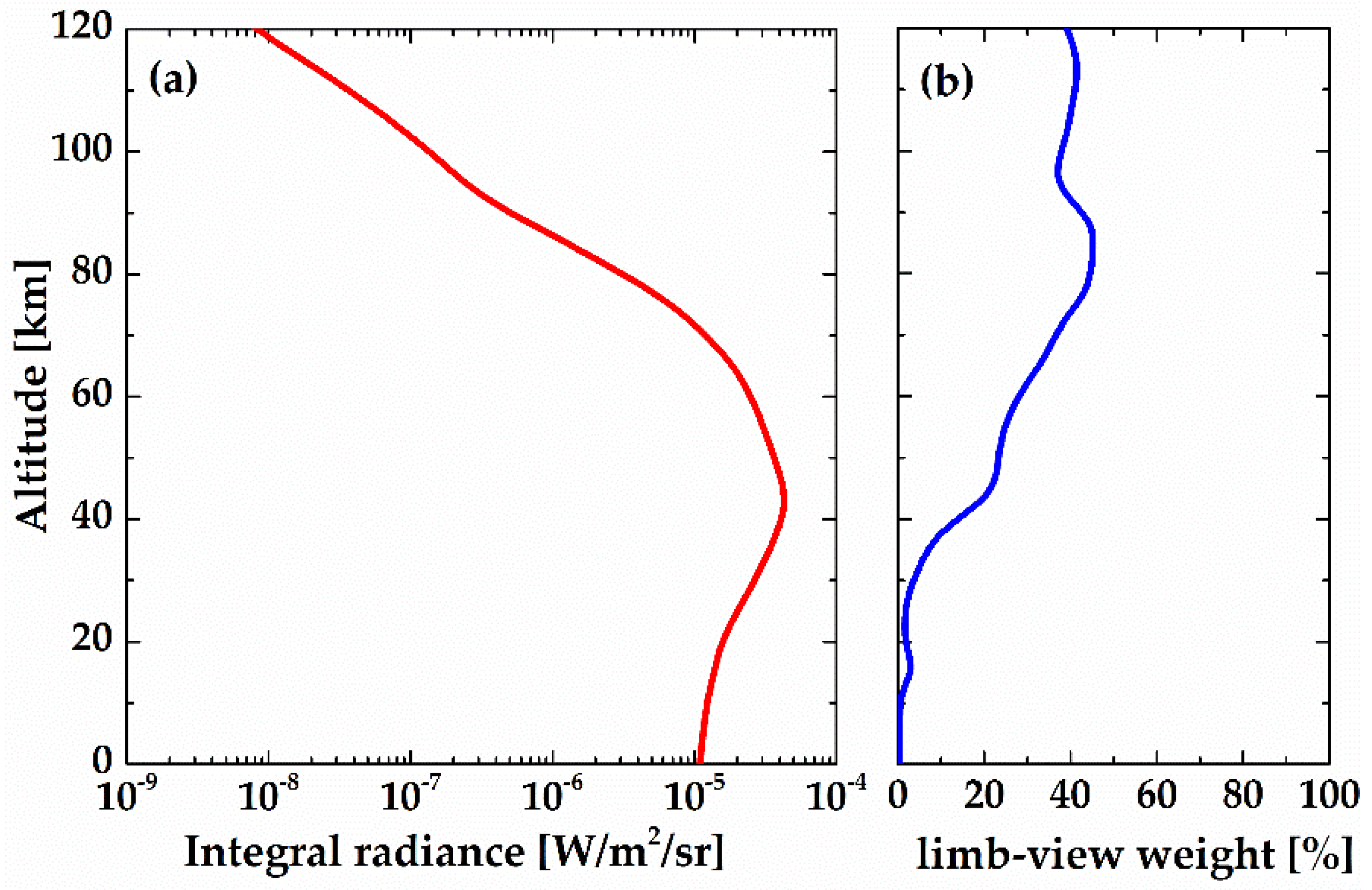
The integral radiance and limb-view weight work together to affect the retrieval accuracy in satellite remote sensing applications. The radiance values and weight profile of the R9Q10 line varying with the tangent altitude are shown in Figure 10. At lower heights, the contribution of the target layer is very small because of the small VER and strong self-absorption. As the tangent height increases, the limb-view weight also increases, which leads to an increase in measurement precision. However, at higher altitudes, the integral radiance goes down exponentially with height, which is certain to cause decrease in the signal-to-noise ratio. Therefore, if the R9Q10 line is used as the target source, the atmospheric information of the tangent point can be obtained from 20 to 90 km, where both the integral radiance and the weight value are large enough.

3.2. Scattering Absorption Spectrum

The brightness spectrum of the O2 infrared atmospheric band scattered by the Earth’s atmosphere is strongly marked by rotational lines of molecular oxygen. Considering source terms reflected by clouds and the Earth’s surface, and scattered by molecules and particles, the limb brightness spectrum with absorption characteristics can be expressed as [24]
I S ( υ , z t ) = [ η s ( υ , s ) + η G ( υ , s ) ] exp [ n ( s ) σ a ( s ) d s ] d s
where
η s ( υ , s ) = Γ ( υ , s ) n a ( s ) σ s ( υ )
Γ ( υ , s ) = Γ ( υ ) exp [ Z ( s ) n ( s ) σ ( s ) D ( υ , s ) d s cos δ ] .
Here, η s ( υ , s ) is the Rayleigh or Mie scattering rate per unit volume, σ s ( υ ) is the total Rayleigh or Mie scattering cross section, Γ ( υ , s ) is the attenuated solar flux, Γ ( υ ) is the top-of-atmosphere solar spectral irradiance, δ is the SZA, and η G ( υ , s ) is the volume scattering rate at the scattering altitude due to ground reflected light. For our study, we adopted the expression of η G ( υ , s ) provided by Hays, et al. [25].
Figure 11 shows the limb spectral radiance of the scattered sunlight at 1.27 μm and the absorbance of the target layer at tangent heights of 40, 60, and 80 km. The spherical adding and doubling methods developed by Abreu, et al. were adopted in this work [26]. As illustrated, the scattered sunlight radiance as well as the absorbance of the target layer goes down exponentially with tangent height. The O2 absorption spectrum is quite similar to limb emission spectrum in shape (shown in Figure 8), while emission lines are much narrower than absorption lines because pressure broadening can be ignored at high altitude. They also have different distributions in spectrum because the emission rate and the absorption cross section are influenced differently by atmospheric temperature due to their different populations of rotational levels (as noted before).
In order to better follow the spectral shape development as a function of tangent height, a close-up of one of these lines (red in Figure 11) is shown in Figure 12 after normalization to the maximum intensity (the asymptotic value). As can be seen, the absorption lines are very broad at tangent heights of 5 and 10 km because of the atmospheric scattering from low altitudes, where collision broadening dominates. At tangent heights higher than 20 km, the whole line shape becomes a superposition of two components: (1) a narrow one, which is sensitive to the atmospheric condition at the tangent point, and (2) a much broader component, which is contributed by the reflection and scattering taking place near the ground and the lower atmosphere.

3.3. Total Spectral Radiance

The spectral brightness that would be observed either in absorption or in emission can be calculated using the above-described airglow emission or scattering absorption radiative transfer models, respectively. The scattering absorption spectrum I S is obtained separately using the line-by-line multiple scattering radiative transfer model. The emission brightness I E is calculated under the assumption that the attenuation along the line-of-sight path is caused by single scattering and self-absorption. Total spectral radiance I T o t a l in both emission and absorption can be obtained by combining these two components together simply because the scattering and emission processes are independent of each other in both physical and mathematical models [27]:
I T o t a l = I E + I S .
The surface characteristics play a key role in determining the line shape of the total spectral brightness for limb observation. Figure 13 shows the asymptotic value and line center intensity as a function of albedos at the tangent height of 15 km. The asymptotic value increases with increasing albedo, while the line center intensity remains the same.
Figure 14 shows the total spectral brightness of the R9Q10 line for albedos equal to 0.2 at different tangent heights. As illustrated, the total spectral brightness can be observed both in absorption and emission, with the latter dominating above 20 km. The O2 infrared atmospheric band line is very broad at low altitudes but observable in narrow emission at higher altitude because thermal motion rather than collision dominates the broadening process. Note that the wings of the line vary significantly with tangent height, both in width and magnitude. The line center, however, develops a peak in the absorption valley. At higher tangent heights (>20 km), the asymptotic value goes down exponentially, but the general shape of the lines remains unchanged.
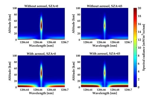
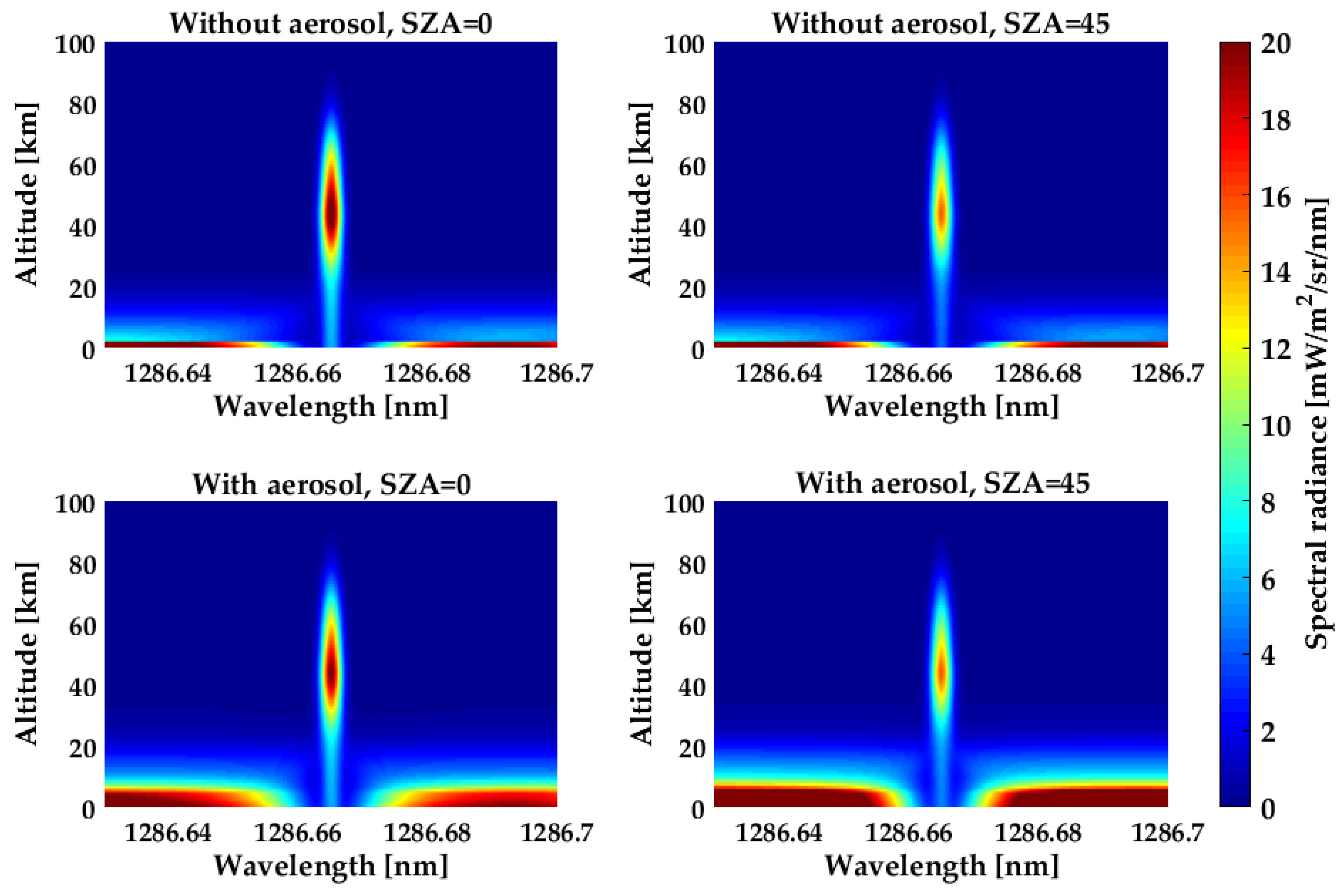
The SZA and atmospheric aerosol have significant influence on both the asymptotic value and line center intensity. Figure 15 shows the variations in total spectral brightness with the SZA and atmospheric aerosol at the tangent heights from 0 to 100 km. Wavelength is the abscissa, tangent height is the ordinate, and the scale of the spectral brightness is made by the pseudo color intensity in each graph. Several features are apparent in this figure. The asymptotic intensity increases by approximately two times when the SZA grows from zero to 45°. The impact of this effect can be explained by Mie and Rayleigh scattering phase functions: scattering angle becomes smaller as the SZA increases, and the decreasing scattering angle leads to an increase in scattered signal. The variation in the line center is not as large as it is in the asymptote. This behavior is due to the fact that the intensity in the line center depends not only on the amount of scattered light but also on absorption and emission. The variation in the SZA changes the path length of the solar radiation passing through, which causes a change in the solar energy being deposited at different heights. As the column densities through the O2 and O3 increase, the optical depth increases, while the photolysis rate decreases. At tangent heights above 80 km, the SZA has a smaller effect on the O2(a1Δg) concentration because of the gradual disappearance of O3. The production of O(1D) becomes the dominant source of O2(a1Δg), and this production steadily decreases with the SZA. The atmospheric aerosol is important in determining the asymptotic intensity. Similar to SZA, the center intensity is not a strong function of the atmospheric aerosol. The center intensity variations with Mie scattering are mostly due to changes in extinction coefficient caused by the existence of aerosol. Changes in the intensity of the absorption feature at low tangent height lines of sight are masked by the dominant emission feature of the mesosphere.
In order to validate the emission–absorption transfer algorithm, we compared our model results with those obtained from MODTRAN4 [28] and the TIMED–SABER measurements [29,30] for the same latitude (48.9°N), date (10 July) and SZA (35.5°). Figure 16a shows the comparison between our model and the MODTRAN4 result at tangent height of 20 km with a surface albedo of 0.2 and an aerosol model of stratospheric background, which validates the multiple scattering algorithm. Due to the resolution limitation of MODTRAN4, the MODTRAN result was calculated at 1 cm−1. The spectral resolution can reach 0.001 cm−1 with our model, in which the multiple scattering algorithm is achieved by means of a line-by-line approach. Figure 16b shows the O2(a1Δg) band brightness calculated by our model and that measured by the TIMED–SABER. The agreement between the observed band brightness and model prediction is remarkable, which suggests that the emission algorithm, including the non-LTE source function and self-absorption calculation, is very sound.

4. Conclusions

We have presented simulations of the radiative transfer characteristics of the O2 infrared atmospheric band in limb-viewing geometry. Both the non-LTE effect and multiple scattering were taken into account for developing the radiative transfer model. This model incorporates the most recent cross sections, spectroscopic parameters, rate constants, and solar fluxes. The limb spectral brightness observed in both absorption and emission was first calculated separately. The scattering absorption spectrum was carried out using the line-by-line multiple scattering radiative transfer model. The emission brightness was calculated based on the non-LTE theory, assuming that the attenuation along the line-of-sight path is caused by single scattering and self-absorption. Total spectral radiance was then obtained by combining these two components together. For the absorption spectrum simulation, the spherical adding and doubling methods were used. In the calculation of emission brightness, the source function under condition of non-LTE was used, which differed greatly from the Planck’s law. The emission rates for calculation of source function were carried out based on six major O2(a1Δg) production mechanisms, and the vibrational temperature was obtained to describe the excitation degree of the excited vibrational state relative to the ground state. The variations in the limb spectral brightness with surface albedo, atmospheric aerosol, and SZA were simulated, and their basic characteristics were discussed. The surface characteristics, SZA, and atmospheric aerosol play key roles in determining the asymptotic value of the line shape, while the line center intensity is just sensitive to changes in atmospheric aerosol and SZA. It is expected that a better understanding of the radiative transfer characteristics of the O2 infrared atmospheric band will certainly improve the accuracy of near-infrared spaceborne instruments, such as WAMI, MIMI, and NWTSI, for which such new knowledge of non-LTE and multiple scattering could be used for an improved retrieval of atmospheric temperature and wind field.

Author Contributions

Conceptualization: W.H., K.W., and Y.F.; methodology: W.H. and K.W.; validation: D.F. and Z.C.; investigation: W.H. and Z.C.; formal analysis: K.W. and F.L.; writing—original draft preparation: W.H. and K.W.; writing—review and editing: Y.F. and F.L.; project administration: Y.F. and K.W.; supervision: F.L. and K.W.; funding acquisition: K.W.

Funding

This research was funded by the National Natural Science Foundation of China (NSFC), grant number 61705253, 41975039.

Acknowledgments

We gratefully acknowledge informative and helpful discussions with Wang Dingyi on theoretical details of this work. We also thank three anonymous reviewers for constructive comments on the initial manuscript.

Conflicts of Interest

The authors declare no conflict of interest.

References

  1. Mlynczak, M.G.; Morgan, F.; Yee, J.H.; Espy, P.; Murtagh, D.; Marshall, B.; Schmidlin, F. Simultaneous measurements of the O2(1∆) and O2(1Σ) airglows and ozone in the daytime mesosphere. Geophys. Res. Lett. 2001, 28, 999–1002. [Google Scholar] [CrossRef]
  2. Khabibrakhmanov, I.K.; Degenstein, D.A.; Llewellyn, E.J. Mesospheric ozone: Determination from orbit with the OSIRIS instrument on Odin. Can. J. Phys. 2002, 80, 493–504. [Google Scholar] [CrossRef]
  3. Mlynczak, M.G.; Marshall, B.T.; Martin-Torres, F.J.; Russell, J.M.; Thompson, R.E.; Remsberg, E.E.; Gordley, L.L. Sounding of the Atmosphere using Broadband Emission Radiometry observations of daytime mesospheric O2(1∆) 1.27 μm emission and derivation of ozone, atomic oxygen, and solar and chemical energy deposition rates. J. Geophys. Res. Atmos. 2007, 112, D15. [Google Scholar] [CrossRef]
  4. Guslyakova, S.; Fedorova, A.A.; Lefèvre, F.; Korablev, O.I.; Montmessin, F.; Bertaux, J.L. O2(1g) dayglow limb observations on Mars by SPICAM IR on Mars-Express and connection to water vapor distribution. Icarus 2014, 239, 131–140. [Google Scholar] [CrossRef]
  5. Ward, W.E.; Gault, W.A.; Shepherd, G.G.; Rowlands, N. The Waves Michelson Interferometer: A visible/near-IR interferometer for observing middle atmosphere dynamics and constituents. Proc. SPIE 2001, 4540, 100–111. [Google Scholar]
  6. He, W.W.; Wu, K.J.; Feng, Y.T.; Fu, D.; Chen, Z.; Li, F.Q. The Near-Space Wind and Temperature Sensing Interferometer: Forward Model and Measurement Simulation. Remote Sens. 2019, 11, 914. [Google Scholar] [CrossRef]
  7. Wu., K.J.; Fu, D.; Feng, Y.T.; Li, J.; Hao, X.B.; Li, F.Q. Simulation and application of the emission line O19P18 of O2(1g) dayglow near 1.27 μm for wind observations from limb-viewing satellites. Opt. Express 2018, 26, 16984–16999. [Google Scholar] [CrossRef]
  8. Park, J.H. Atmospheric CO2 monitoring from space. Appl. Opt. 1997, 36, 2701–2712. [Google Scholar] [CrossRef]
  9. Kang, S.; Gordon, I.E.; Sioris, C.E.; Xiong, L.; Chance, K.; Wofsy, S.C. Reevaluating the use of O2(1g) band in spaceborne remote sensing of greenhouse gases. Geophys. Res. Lett. 2018, 45, 5779–5787. [Google Scholar]
  10. Dobler, J.T.; F Wallace, H.; Browell, E.V.; Bing, L.; Doug, M.G.; Susan, K.; Yonghoon, C.; Syed, I. Atmospheric CO2 column measurements with an airborne intensity-modulated continuous wave 1.57 μm fiber laser lidar. Appl. Opt. 2013, 52, 2874–2892. [Google Scholar] [CrossRef]
  11. Sharp, W.E.; Zaccheo, T.S.; Browell, E.V.; Ismail, S.; Dobler, J.T.; Llewellyn, E.J. Impact of Ambient O2(1g) on Satellite-Based Laser Remote Sensing of O2 Columns using Absorption Lines in the 1.27 µm region. J. Geophys. Res. Atmos. 2014, 119, 7757–7772. [Google Scholar] [CrossRef]
  12. Bertaux, J.L.; Hauchecorne, A.; Lefèvre, F.; Bréon, F.M.; Blanot, L.; Jouglet, D.; Lafrique, P.; Akaev, P. The use of O2 1.27 µm absorption band revisited for GHG monitoring from space and application to MicroCarb. Atmos. Meas. Tech. Discuss. 2019. in review. [Google Scholar] [CrossRef]
  13. Gordon, I.E.; Rothman, L.S.; Hill, C.; Kochanov, R.V.; Tan, Y.; Bernath, P.F.; Birk, M.; Boudon, V.; Campargue, A.; Chance, K.V.; et al. The HITRAN2016 molecular spectroscopic database. J. Quant. Spectrosc. Radiat. Transf. 2017, 203, 3–69. [Google Scholar] [CrossRef]
  14. Mlynczak, M.G.; Solomon, S.; Zaras, D.S. An updated model for O2(1g) concentrations in the mesosphere and lower thermosphere and implications for remote sensing of ozone at 1.27 μm. J. Geophys. Res. Atmos. 1993, 98, 18639–18648. [Google Scholar] [CrossRef]
  15. Thomas, R.J.; Barth, C.A.; Rusch, D.W.; Rusch, D.W.; Sanders, R.W. Solar Mesosphere Explorer near-infrared spectrometer: Measurements of 1.27-μm radiances and the inference of mesospheric ozone. J. Geophys. Res. Atmos. 1984, 89, 9569–9580. [Google Scholar] [CrossRef]
  16. Harris, R.D.; Adams, G.W. Where does the O(1D) energy go? J. Geophys. Res. Space 1983, 88, 4918–4928. [Google Scholar] [CrossRef]
  17. Yankovsky, V.A.; Babaev, A.S. Photolysis of O3 at Hartley, Chappuis, Huggins, and Wulf bands in the middle atmosphere: Vibrational kinetics of oxygen molecules O2 (X3 Σg, ν ≤ 35). Atmos. Ocean. Opt. 2011, 24, 6–16. [Google Scholar] [CrossRef]
  18. Yankovsky, V.A.; Manuilova, R.; Babaev, A.; Feofilov, A.; Kutepov, A. Model of electronic-vibrational kinetics of the O3 and O2 photolysis products in the middle atmosphere: Applications to water vapour retrievals from SABER/TIMED 6.3 µm radiance measurements. Int. J. Remote Sens. 2011, 32, 3065–3078. [Google Scholar] [CrossRef]
  19. Martyshenko, K.V.; Yankovsky, V.A. IR band of O2 at 1.27 μm as the tracer of O3 in the mesosphere and lower thermosphere: Correction of the method. Geomagn. Aeron. 2017, 57, 229–241. [Google Scholar] [CrossRef]
  20. Yankovsky, V.A.; Manuilova, R.O. Model of daytime emissions of electronically-vibrationally excited products of O3 and O2 photolysis: Application to ozone retrieval. Ann. Geophys. 2006, 24, 2823–2839. [Google Scholar] [CrossRef]
  21. Russell, J.P.; Lowe, R.P. Atomic oxygen profiles (80–94 km) derived from Wind Imaging Interferometer/Upper Atmospheric Research Satellite measurements of the hydroxyl airglow: 1. Validation of technique. J. Geophys. Res. 2003, 108, 4662. [Google Scholar] [CrossRef]
  22. Yankovsky, V.; Vorobeva, E.; Manuilova, R. New techniques for retrieving the [O(3P)], [O3] and [CO2] altitude profiles from dayglow oxygen emissions: Uncertainty analysis by the Monte Carlo method. Adv. Space Res. 2019, 64, 1948–1967. [Google Scholar] [CrossRef]
  23. Edwards, D.P.; Lopez-Puertas, M.; Lopez-Valverde, M.A. Non-local thermodynamic equilibrium studies of the 15-μm bands of CO2 for atmospheric remote sensing. J. Geophys. Res. Atmos. 1993, 98, 14955–14977. [Google Scholar] [CrossRef]
  24. Hays, P.B. High-resolution optical measurements of atmospheric winds from space. 1: Lower atmosphere molecular absorption. Appl. Opt. 1982, 21, 1136–1141. [Google Scholar] [CrossRef] [PubMed]
  25. Hays, P.B.; Abreu, V.J. Absorption line profiles in a moving atmosphere—A single scattering linear perturbation theory. J. Geophys. Res. Atmos. 1989, 94, 18351–18365. [Google Scholar] [CrossRef]
  26. Abreu, V.J.; Bucholtz, A.; Hays, P.B.; Ortland, D.; Skinner, W.R.; Yee, J.H. Absorption and emission line shapes in the 02 atmospheric bands: Theoretical model and limb viewing simulations. Appl. Opt. 1989, 28, 2128–2137. [Google Scholar] [CrossRef]
  27. Yee, J.H.; DeMajistre, R.; Morgan, F. The O2(b1Σ) dayglow emissions: Application to middle and upper atmosphere remote sensing. Can. J. Phys. 2012, 90, 769–784. [Google Scholar] [CrossRef]
  28. Anderson, G.P.; Berk, A.; Acharya, P.K.; Matthew, M.W.; Bernstein, L.S.; Chetwynd, J.H.J.; Dothe, H.; Adler-Golden, S.M.; Ratkowski, A.J.; Felde, G.W.; et al. MODTRAN4: Radiative transfer modeling for remote sensing. Proc. SPIE 2000, 4049, 176–183. [Google Scholar]
  29. SABER—Sounding of the Atmosphere using Broadband Emission Radiometry. Available online: http://saber.gats-inc.com/ (accessed on 30 October 2019).
  30. Mlynczak, M.G.; Russell, J.M. An overview of the SABER experiment for the TIMED mission. Opt. Remote Sens. Atmos. 1995, 2, 5–7. [Google Scholar]
Figure 1. The absorption line strength and spectral distribution of the O2 infrared atmospheric band and the O2 atmospheric band (from HITRAN [13]).
Remotesensing 11 02702 g001
Figure 2. Dayglow production mechanism of the O2 infrared atmospheric band [20].
Remotesensing 11 02702 g002
Figure 3. The modeled O2(a1Δg) concentration profile and respective contributions of each production mechanism.
Remotesensing 11 02702 g003
Figure 4. The calculated relative contribution of O2(a1Δg) molecules at ν = 0 , ν = 1 , and ν = 2 as a function of altitude.
Remotesensing 11 02702 g004
Figure 5. The calculated volume emission rate (VER) profiles of the O2(a1Δg) dayglow in the four seasons.
Remotesensing 11 02702 g005
Figure 6. (a) The emission and absorption spectrum as a function of the transition wavelength. (b) The ratio of emission to absorption line strength for each line.
Remotesensing 11 02702 g006
Figure 7. The construction of the path model in limb-viewing geometry.
Remotesensing 11 02702 g007
Figure 8. The calculated limb spectral brightness and the spectral radiance of the target layer at different tangent heights.
Remotesensing 11 02702 g008
Figure 9. The spectral brightness of line R9Q10 with and without self-absorption as well as its atmospheric transmission at 50 km tangent height.
Remotesensing 11 02702 g009
Figure 10. The integral radiance (a) and limb-view weight (b) of the R9Q10 line varying with the tangent altitude.
Remotesensing 11 02702 g010
Figure 11. The limb spectral radiance of the scattered sunlight at 1.27 μm and the absorbance of the target layer at different tangent heights.
Remotesensing 11 02702 g011
Figure 12. Variation in the absorption line shape with tangent heights. The line shape is broad at lower tangent heights of 5 and 10 km and becomes a superposition of a narrow component and a much broader one above 20 km.
Remotesensing 11 02702 g012
Figure 13. The line shape of the total spectral brightness as a function of albedos at the tangent height of 15 km.
Remotesensing 11 02702 g013
Figure 14. The total spectral brightness of the R9Q10 line varying with tangent heights.
Remotesensing 11 02702 g014
Figure 15. The variations in total spectral brightness with the solar zenith angle (SZA) and atmospheric aerosol at the tangent heights from 0 to 100 km.
Remotesensing 11 02702 g015
Figure 16. Comparisons between the emission–absorption transfer model and results from MODTRAN4 and the TIMED–SABER measurements. (a) Calculated spectral radiance using our model and MODTRAN4 at tangent height of 20 km. (b) Measured and modeled O2(a1Δg) band brightness as a function of tangent height.
Remotesensing 11 02702 g016

