Spatiotemporal Fusion of Satellite Images via Very Deep Convolutional Networks


Abstract
:
1. Introduction
2. Related Work
2.1. Convolutional Neural Networks (CNNs)
2.2. CNNs for Single-Image Super-Resolution
3. Methodology
3.1. Configurations of Non-Linear Mapping VDCN
3.2. Configurations of Super-Resolution VDCN
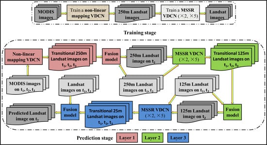
3.3. Training Networks
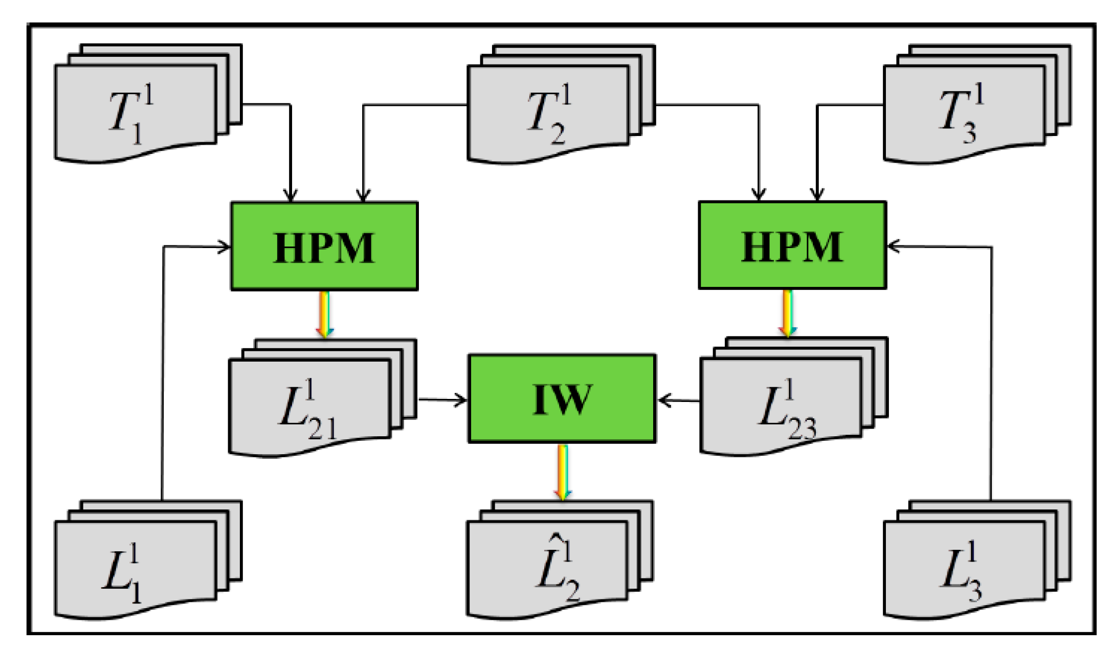
3.4. Three-Layer Prediction Step
4. Experimental Results
4.1. Sites and Datasets
4.2. Quantitative Evaluation Indices
4.3. Experimental Setting
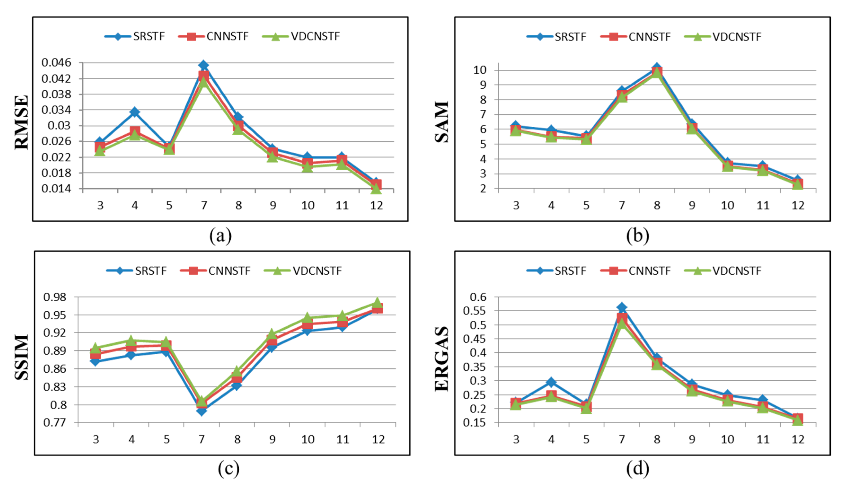
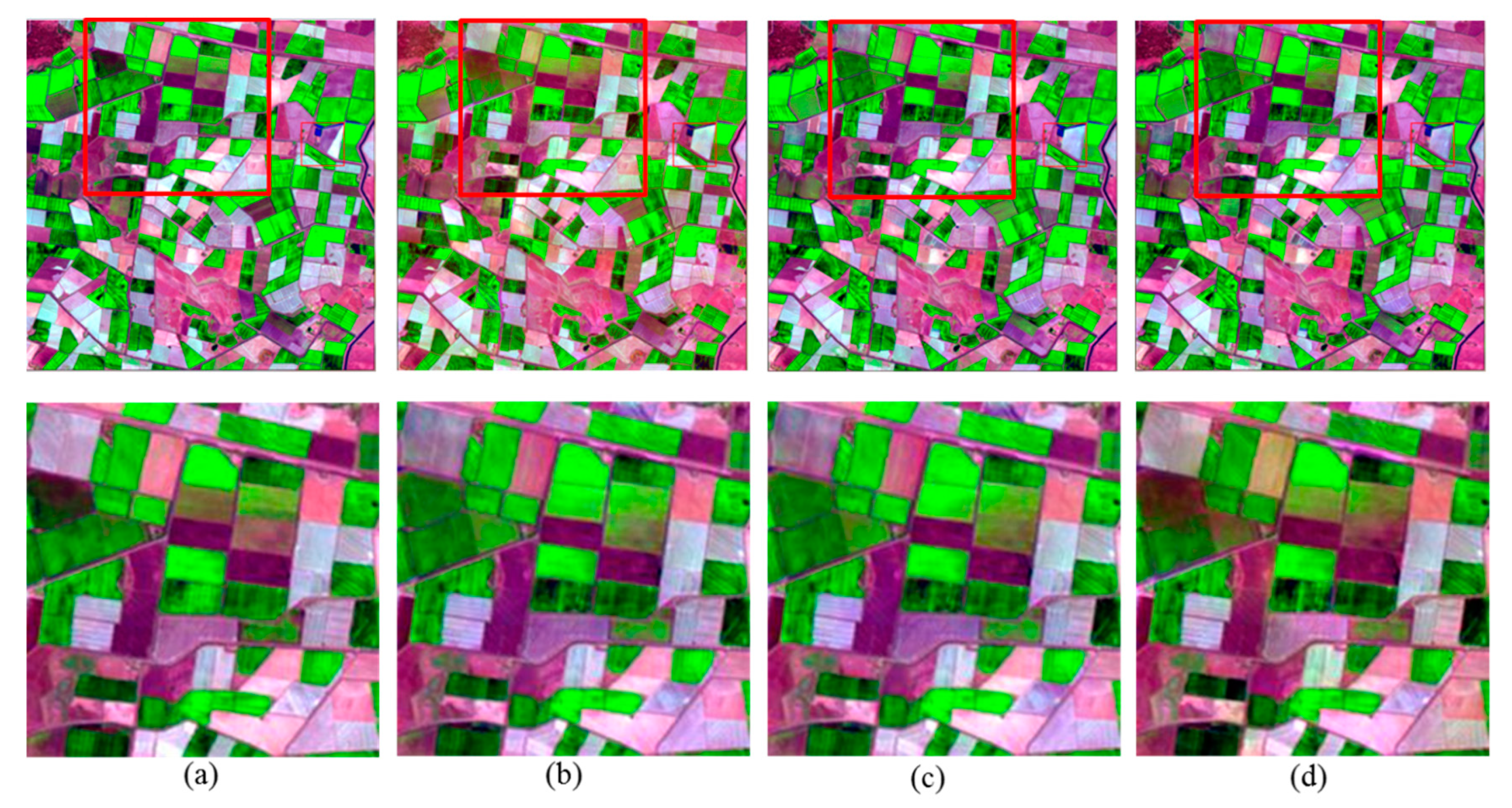
4.4. Experimental Results
5. Discussion
6. Conclusions
Author Contributions
Funding
Acknowledgments
Conflicts of Interest
References
- Zhou, J.; Khot, L.R.; Boydston, R.A.; Miklas, P.N.; Porter, L. Low altitude remote sensing technologies for crop stress monitoring: a case study on spatial and temporal monitoring of irrigated pinto bean. Precision Agric. 2018, 19, 555–569. [Google Scholar] [CrossRef]
- Dang, L.M.; Hassan, S.I.; Suhyeon, I.; Sangaiah, A.K.; Mehmood, I.; Rho, S.; Seo, S.; Moon, H.; Syed, I.H. UAV based wilt detection system via convolutional neural networks. Sustain. Comput. Inform. Syst. 2018. [Google Scholar] [CrossRef]
- Schwaller, M.; Hall, F.; Gao, F.; Masek, J. On the blending of the Landsat and MODIS surface reflectance: predicting daily Landsat surface reflectance. IEEE Trans. Geosci. Remote. Sens. 2006, 44, 2207–2218. [Google Scholar]
- Hilker, T.; Wulder, M.A.; Coops, N.C.; Linke, J.; McDermid, G.; Masek, J.G.; Gao, F.; White, J.C. A new data fusion model for high spatial- and temporal-resolution mapping of forest disturbance based on Landsat and MODIS. Remote. Sens. Environ. 2009, 113, 1613–1627. [Google Scholar] [CrossRef]
- Zhu, X.; Chen, J.; Gao, F.; Chen, X.; Masek, J.G. An enhanced spatial and temporal adaptive reflectance fusion model for complex heterogeneous regions. Remote. Sens. Environ. 2010, 114, 2610–2623. [Google Scholar] [CrossRef]
- Wang, Q.; Zhang, Y.; Onojeghuo, A.O.; Zhu, X.; Atkinson, P.M. Enhancing Spatio-Temporal Fusion of MODIS and Landsat Data by Incorporating 250 m MODIS Data. IEEE J. Sel. Top. Appl. Earth Obs. Remote. Sens. 2017, 10, 4116–4123. [Google Scholar] [CrossRef]
- Acerbi-Junior, F.; Clevers, J.; Schaepman, M. The assessment of multi-sensor image fusion using wavelet transforms for mapping the Brazilian Savanna. Int. J. Appl. Earth Obs. Geoinf. 2006, 8, 278–288. [Google Scholar] [CrossRef]
- Song, H.; Huang, B. Spatiotemporal Reflectance Fusion via Sparse Representation. IEEE Trans. Geosci. Remote. Sens. 2012, 50, 3707–3716. [Google Scholar]
- Song, H.; Huang, B. Spatiotemporal satellite image fusion through one-pair image learning. IEEE Trans. Geosci. Remote. Sens. 2013, 51, 1883–1896. [Google Scholar] [CrossRef]
- Song, H.; Liu, Q.; Wang, G.; Hang, R.; Huang, B. Spatiotemporal Satellite Image Fusion Using Deep Convolutional Neural Networks. IEEE J. Sel. Top. Appl. Earth Obs. Remote. Sens. 2018, 11, 821–829. [Google Scholar] [CrossRef]
- Zhu, X.; Cai, F.; Tian, J.; Williams, T.K.-A. Spatiotemporal Fusion of Multisource Remote Sensing Data: Literature Survey, Taxonomy, Principles, Applications, and Future Directions. Remote. Sens. 2018, 10, 527. [Google Scholar]
- LeCun, Y.; Boser, B.; Denker, J.S.; Henderson, D.; Howard, R.E.; Hubbard, W.; Jackel, L.D. Backpropagation Applied to Handwritten Zip Code Recognition. Neural Comput. 1989, 1, 541–551. [Google Scholar] [CrossRef]
- Zeiler, M.D.; Fergus, R. Visualizing and Understanding Convolutional Networks. In Proceedings of the Model and Data Engineering; Springer Science and Business Media LLC: Berlin/Heidelberg, Germany, 2014; Volume 8689, pp. 818–833. [Google Scholar]
- Nair, V.; Hinton, G.E. Rectified linear units improve restricted boltzmann machines. In Proceedings of the 27th International Conference on International Conference on Machine Learning, Haifa, Israel, 21–24 June 2010; pp. 807–814. [Google Scholar]
- Ioffe, S.; Szegedy, C. Batch normalization: Accelerating deep network training by reducing internal covariate shift. In Proceedings of the 32nd International Conference on International Conference on Machine Learning, Lille, France, 6–11 July 2015; pp. 448–456. [Google Scholar]
- He, K.; Zhang, X.; Ren, S.; Sun, J. Deep Residual Learning for Image Recognition. In Proceedings of the 2016 IEEE Conference on Computer Vision and Pattern Recognition (CVPR), Las Vegas, NV, USA, 26 June–1 July 2016; pp. 770–778. [Google Scholar]
- Jain, V.; Seung, H.S. Natural image denoising with convolutional networks. In Proceedings of the Advances in Neural Information Processing Systems, Vancouver, BC, Canada, 8–10 December 2008; pp. 769–776. [Google Scholar]
- Dong, C.; Loy, C.C.; He, K.; Tang, X. Image super-resolution using deep convolutional networks. IEEE Trans. Pattern Anal. Mach. Intell. 2016, 38, 295–307. [Google Scholar] [CrossRef] [PubMed]
- Girshick, R.; Donahue, J.; Darrell, T.; Malik, J. Rich feature hierarchies for accurate object detection and semantic segmentation. In Computer Vision and Pattern Recognition; CVPR: Piscataway, NJ, USA, 2013; pp. 580–587. [Google Scholar]
- Krizhevsky, A.; Sutskever, I.; Hinton, G.E. Imagenet classification with deep convolutional neural networks. In Proceedings of the International Conference on Neural Information Processing Systems, Lake Tahoe, NV, USA, 3–6 December 2012; pp. 1097–1105. [Google Scholar]
- Simonyan, K.; Zisserman, A. Very Deep Convolutional Networks for Large-Scale Image Recognition. arXiv 2014, arXiv:1409.1556. Available online: https://arxiv.org/pdf/1409.1556.pdf (accessed on 11 October 2019).
- Yang, J.; Wright, J.; Huang, T.S.; Ma, Y. Image Super-Resolution Via Sparse Representation. IEEE Trans. Image Process. 2010, 19, 2861–2873. [Google Scholar] [CrossRef] [PubMed]
- Kim, J.; Lee, J.K.; Lee, K.M. Accurate image super-resolution using very deep convolutional networks. In Proceedings of the IEEE Conference on Computer Vision and Pattern Recognition, Las Vegas, NV, USA, 26 June–1 July 2016; pp. 1646–1654. Available online: https://arxiv.org/pdf/1511.04587.pdf (accessed on 11 October 2019).
- Tuna, C.; Ünal, G.; Sertel, E. Single-frame super resolution of remote-sensing images by convolutional neural networks. Int. J. Remote. Sens. 2018, 39, 2463–2479. [Google Scholar] [CrossRef]
- Pouliot, D.; Latifovic, R.; Pasher, J.; Duffe, J. Landsat Super-Resolution Enhancement Using Convolution Neural Networks and Sentinel-2 for Training. Remote. Sens. 2018, 10, 394. [Google Scholar] [CrossRef]
- Timofte, R.; Smet, V.D.; Gool, L.V. A+: Adjusted anchored neighborhood regression for fast super-resolution. In Proceedings of the Asian Conference on Computer Vision, Singapore, 1–5 November 2014; pp. 111–126. [Google Scholar]
- Jia, X.; Xu, X.; Cai, B.; Guo, K. Single image super-resolution using multi-scale convolutional neural network. In Proceedings of the IEEE Conference on Computer Vision and Pattern Recognition, Honolulu, HI, USA, 21–26 July 2017; Available online: https://arxiv.org/pdf/1705.05084.pdf (accessed on 11 October 2019).
- LeCun, Y.; Bottou, L.; Bengio, Y.; Haffner, P. Gradient-based learning applied to document recognition. Proc. IEEE 1998, 86, 2278–2324. [Google Scholar] [CrossRef]
- Emelyanova, I.V.; Mcvicar, T.R.; Niel, T.G.V.; Li, L.T.; van Dijk, A.I.J.M. Assessing the accuracy of blending landsatcmodis surface reflectances in two landscapes with contrasting spatial and temporal dynamics: A framework for algorithm selection. Remote Sens. Environ. 2013, 133, 193–209. [Google Scholar] [CrossRef]
- Berk, A.; Anderson, G.P.; Bernstein, L.S.; Acharya, P.K.; Dothe, H.; Matthew, M.W.; Adler-Golden, S.M.; Chetwynd, J.J.H.; Richtsmeier, S.C.; Pukall, B.; et al. MODTRAN4 radiative transfer modeling for atmospheric correction. SPIE’s Int. Symp. Opt. Sci. Engin. Instrum. 1999, 3756, 348. [Google Scholar]
- Jupp, D.L.B.; Reddy, S.; Lymburner, L.; Mueller, N.; Islam, A.; Li, F.; Tan, P. An Evaluation of the Use of Atmospheric and BRDF Correction to Standardize Landsat Data. IEEE J. Sel. Top. Appl. Earth Obs. Remote. Sens. 2010, 3, 257–270. [Google Scholar]
- Yuhas, R.; Goetz, A.F.H.; Boardman, J.W. Descrimination among Semi-Arid Landscape Endmembers Using the Spectral Angle Mapper (SAM) Algorithm. JPL. 1992. Available online: https://aviris.jpl.nasa.gov/proceedings/workshops/92_docs/52.PDF (accessed on 11 October 2019).
- Wang, Z.; Bovik, A.; Sheikh, H.; Simoncelli, E. Image Quality Assessment: From Error Visibility to Structural Similarity. IEEE Trans. Image Process. 2004, 13, 600–612. [Google Scholar] [CrossRef] [PubMed]
- Khan, M.; Alparone, L.; Chanussot, J. Pansharpening Quality Assessment Using the Modulation Transfer Functions of Instruments. IEEE Trans. Geosci. Remote. Sens. 2009, 47, 3880–3891. [Google Scholar] [CrossRef]


| CIA | LGC | |
|---|---|---|
| Network depth for NLM-VDCN 3 | 15 | |
| Network depth for MSSR-VDCN4 | 20 | |
| Size of training sub-images for NLM-VDCN | 31 | |
| Size of training sub-images for MSSR-VDCN | 41 | |
| Size of training batches | 64 | |
| Interpolation method 5 | Bicubic | |
| Loss function | Mean squared error | |
| Number of training samples for NLM-VDCN | 25,344 | 49,920 |
| Number of training samples for MSSR-VDCN | 137,472 | 315,648 |
| Initial learning rate | 0.01 | |
| Momentum | 0.9 | |
| weight decay | 0.0001 | |
| Epochs | 80 | |
| Index | Bands | SRSTF | CNNSTF | VDCNSTF |
|---|---|---|---|---|
| RMSE | B1 | 0.0093 | 0.0073 | 0.0059 |
| B2 | 0.0115 | 0.0112 | 0.0105 | |
| B3 | 0.0184 | 0.0143 | 0.0133 | |
| B4 | 0.0251 | 0.0222 | 0.0219 | |
| B5 | 0.0267 | 0.0231 | 0.0220 | |
| B6 | 0.0239 | 0.0213 | 0.0193 | |
| SAM | 2.6879 | 2.3393 | 2.2993 | |
| SSIM | B1 | 0.9679 | 0.9775 | 0.9835 |
| B2 | 0.9647 | 0.9700 | 0.9748 | |
| B3 | 0.9423 | 0.9556 | 0.9610 | |
| B4 | 0.9205 | 0.9309 | 0.9337 | |
| B5 | 0.9059 | 0.9175 | 0.9228 | |
| B6 | 0.8986 | 0.9096 | 0.9150 | |
| ERGAS | 0.2325 | 0.2026 | 0.1986 |
| Index | Bands | SRSTF | CNNSTF | VDCNSTF |
|---|---|---|---|---|
| RMSE | B1 | 0.0152 | 0.0141 | 0.0133 |
| B2 | 0.0203 | 0.0195 | 0.0185 | |
| B3 | 0.0256 | 0.0246 | 0.0236 | |
| B4 | 0.0344 | 0.0317 | 0.0305 | |
| B5 | 0.0542 | 0.0514 | 0.0502 | |
| B6 | 0.0426 | 0.0389 | 0.0381 | |
| SAM | 10.1531 | 9.8586 | 9.8086 | |
| SSIM | B1 | 0.9372 | 0.9482 | 0.9583 |
| B2 | 0.9178 | 0.9284 | 0.9383 | |
| B3 | 0.8948 | 0.9042 | 0.9143 | |
| B4 | 0.8517 | 0.8589 | 0.8690 | |
| B5 | 0.6741 | 0.6916 | 0.7016 | |
| B6 | 0.7135 | 0.7401 | 0.7501 | |
| ERGAS | 0.3801 | 0.3622 | 0.3572 |
© 2019 by the authors. Licensee MDPI, Basel, Switzerland. This article is an open access article distributed under the terms and conditions of the Creative Commons Attribution (CC BY) license (http://creativecommons.org/licenses/by/4.0/).
Share and Cite
Zheng, Y.; Song, H.; Sun, L.; Wu, Z.; Jeon, B. Spatiotemporal Fusion of Satellite Images via Very Deep Convolutional Networks. Remote Sens. 2019, 11, 2701. https://doi.org/10.3390/rs11222701
Zheng Y, Song H, Sun L, Wu Z, Jeon B. Spatiotemporal Fusion of Satellite Images via Very Deep Convolutional Networks. Remote Sensing. 2019; 11(22):2701. https://doi.org/10.3390/rs11222701
Chicago/Turabian StyleZheng, Yuhui, Huihui Song, Le Sun, Zebin Wu, and Byeungwoo Jeon. 2019. "Spatiotemporal Fusion of Satellite Images via Very Deep Convolutional Networks" Remote Sensing 11, no. 22: 2701. https://doi.org/10.3390/rs11222701
APA StyleZheng, Y., Song, H., Sun, L., Wu, Z., & Jeon, B. (2019). Spatiotemporal Fusion of Satellite Images via Very Deep Convolutional Networks. Remote Sensing, 11(22), 2701. https://doi.org/10.3390/rs11222701