Article

Fine-Grained Classification of Hyperspectral Imagery Based on Deep Learning

1
School of Electronics and Information Engineering, Harbin Institute of Technology, Harbin 150001, China
2
RIKEN Center for Advanced Intelligence Project, Tokyo 103-0027, Japan
3
School of Engineering and Information Technology, The University of New South Wales, Canberra, ACT 2600, Australia
*
Author to whom correspondence should be addressed.
Remote Sens. 2019, 11(22), 2690; https://doi.org/10.3390/rs11222690
Submission received: 16 October 2019 / Revised: 13 November 2019 / Accepted: 13 November 2019 / Published: 18 November 2019
(This article belongs to the Special Issue Deep Learning and Feature Mining Using Hyperspectral Imagery)

Abstract

:
Hyperspectral remote sensing obtains abundant spectral and spatial information of the observed object simultaneously. It is an opportunity to classify hyperspectral imagery (HSI) with a fine-grained manner. In this study, the fine-grained classification of HSI, which contains a large number of classes, is investigated. On one hand, traditional classification methods cannot handle fine-grained classification of HSI well; on the other hand, deep learning methods have shown their powerfulness in fine-grained classification. So, in this paper, deep learning is explored for HSI supervised and semi-supervised fine-grained classification. For supervised HSI fine-grained classification, densely connected convolutional neural network (DenseNet) is explored for accurate classification. Moreover, DenseNet is combined with pre-processing technique (i.e., principal component analysis or auto-encoder) or post-processing technique (i.e., conditional random field) to further improve classification performance. For semi-supervised HSI fine-grained classification, a generative adversarial network (GAN), which includes a discriminative CNN and a generative CNN, is carefully designed. The GAN fully uses the labeled and unlabeled samples to improve classification accuracy. The proposed methods were tested on the Indian Pines data set, which contains 33,3951 samples with 52 classes. The experimental results show that the deep learning-based methods provide great improvements compared with other traditional methods, which demonstrate that deep models have huge potential for HSI fine-grained classification.

1. Introduction

Hyperspectral imaging obtains data of the observing target with spectral and spatial information simultaneously and has become a useful tool for a wide branch of users. Among the hyperspectral imagery (HSI) processing methods, classification is one of the core techniques, which tries to allocate a specific class to each pixel in the scene. HSI classification is widely-used including urban development, land change monitoring, scene interpretation, and resource management [1].
The data acquisition capability of remote sensing has been largely improved in the recent decades. In the context of hyperspectral remote sensing, varieties of instruments will be available for Earth observation. Those advanced technologies have increased different types of satellites images which have different resolutions in spectral and spatial dimensions. In general, it leads to difficulties and also opportunities for data processing techniques [2].
In common, the data shown in hyperspectral remote sensing have following features: abundant of object labels, a large size of pixels, and high dimensional features. To the best of our knowledge, most of hyperspectral datasets do not contain more than 20 classes individually. How to handle HSI classification with a large number of classes is a challenging task in real applications. In this study, we investigate the classification of Indian Pines dataset which contains 52 classes. As far as we can see, it is the only public dataset with more than 50 classes. Furthermore, for the Indian Pines dataset, there are fine-grained classes which contain more specific and detailed information compared with the traditional coarse definition of classes.
Among the HSI processing techniques, classification is one of the most vibrant topics. There are three types of HSI classification methods: supervised, unsupervised, and semi-supervised ones. Most of the existing HSI classifiers are based on supervised learning methods.
Due to the abundant spectral information of HSI, traditional methods have been focused on spectral classifiers including multinomial logistic regression [3], random forest [4], neural network [5], support vector machine [6,7], sparse representation [8], and deep learning [9,10,11].
HSI contains both spectral and spatial information. With the help of spatial information, the classification performance can be significantly improved. Therefore, spectral-spatial classifiers are the mainstream of supervised HSI classification [12]. Typical spectral-spatial classification techniques are based on morphological profiles [13,14], multiple kernels [15], and sparse representation [8]. Morphological profile and its extensions extract the spatial features of HSI, and support vector machines (SVMs) or random forests are followed to obtain the final classification map [16,17]. On the other hand, multiple kernel-based methods use different kernels to handle the heterogeneous spectral and spatial features in an efficient manner [18]. In sparse representation-based methods, spatial information is incorporated to formulate spectral-spatial classifiers [8].
The collection of labeled training samples is costly and time-consuming. Therefore, the number of training samples is usually limited in practice. On the other hand, there are many unlabeled samples in the dataset. The semi-supervised classification, which uses the labeled and unlabeled samples together is a promising way to solve the problem of limited training samples [19,20,21]. A transductive support vector machine has been introduced to classify remote sensing images [22]. The proposed transductive SVM significantly increased the classification accuracy compared to the standard SVM. In [23], the semi-supervised graph-based method, which combined composite kernels, has been developed for hyperspectral image classification. Although the number of publications of semi-supervised classification in the literature is smaller than that of supervised learning, it is very important in remote sensing applications.
The aforementioned supervised and semi-supervised methods do not classify HSI in a “deep” manner. Deep learning-based models have the advantages in feature extraction, which have shown their capability in many research areas computer vision [24], speech recognition [25], machine translation [26], and remote sensing [27,28].
Most of popular deep learning models, including stacked auto-encoder [29,30], deep belief network [12,31], convolutional neural network (CNN) [32,33,34,35], and recurrent neural network [36], have been explored for HSI classification. Among the aforementioned deep models, CNN-based methods are widely-used for HSI classification. Similar works for the purpose of extracting spectral-spatial features from pixel have been proposed using a deep CNN in [37]. Li et al. [38] leverage the CNN method to extract pixel-pairs features of HSI following by a majority voting strategy to predict the final classification result. Z. Zhong et al. proposed a 3D-deep network which receives 3D-blocks equipped with spatial and spectral information both from HSI and calculates 3D-convolution kernels for each pixel [39]. In [40], a light 3D-convolution was proposed for extracting the deep spectral-spatial-combined features and the proposed model was less likely to overfitting and easy to train. Furthermore, in [41], band selection was used to select informative and discriminative bands, and then the labeled and unlabeled samples were fed into a 3D-convolutional Auto-Encoder to get the encoded features for semi-supervised HSI classification. In the meanwhile, Romero et al. [34] raised an unsupervised deep CNN to grab sparse features for the limitation of a small training set. In 2018, generative adversarial network (GAN) was used as a supervised classification method to obtain accurate classification of HSI [42], and in [43] a semi-supervised classification utilizing spectral features based on GAN was proposed.
Although deep learning-based methods have shown their capability in HSI processing, deep learning is still in the early stage for HSI classification. There are many specific classification problems, including few training samples and HSI with a great number of classes, to be solved by deep learning methods.
Fine-grained classification tries to classify data with small diversity of relatively large number of classes. Few methods have been proposed for HSI fine-grained classification. As far as we know, only in [44], SVM was used to classify HSI with a great number of classes. How to classify HSI with volume and variety is an urgent task to be tackled nowadays. Due to the advantages of deep learning, it is necessary to use deep learning methods for HSI fine-grained classification.
Furthermore, due to the difficulty and time-consuming to label samples, labeled training samples are usually limited. It is necessary to use the unlabeled samples, which can be used to improve the classification performance.
Moreover, the processing time is another important factor of practical applications. As we know, HSI classification with lots of training samples is time-consuming. In order to speed up the classification procedure, preprocessing of HSI, which reduces the computational complexity of classification, is usually needed. On one hand, these preprocessing techniques are traditionally performed through spectral dimensionality reduction algorithms (e.g., principal component analysis (PCA) [45] and Auto-Encoder (AE)). On the other hand, the deep learning methods which are the combinations of feature extraction and classification, can reduce the classification time via the feature extraction stage. In [30,46], the new spectral-spatial HSI classification methods based on the deep features extraction using stacked-auto-encoders (SAE) are proposed, which have achieved an effective performance on HSI classification.
Generally speaking, a further refinement process can produce an improved classification output. Considering that, some post-processing methods combining probabilistic graphical models such as MRF and conditional random field (CRF) with CNN have been explored in [47,48]. For example, Liu et al. [49] used CRF to improve the segmentation outputs by explicitly modeling the contextual information between regions. Furthermore, Chen et al. [50] proposed a fully connected Gaussian CRF model with respective unary potentials getting from a CNN instead of using a disconnected approach. And Zheng et al. [51] demonstrated a dense CRF with Gaussian pairwise potentials as a recurrent neural network to improve the low-resolution prediction by a traditional CNN.
In this study, the deep learning-based methods for hyperspectral supervised and semi-supervised fine-grained classification are investigated. With the help of deep learning models, the proposed methods achieve significant improvements in terms of classification accuracy. Besides, compared with traditional methods like SVM-based methods, the deep learning models can reduce the total running time (e.g., training and test time). In more details, the main contributions of this study are summarized as follows.
(1) The deep learning-based methods are explored for supervised and semi-supervised fine-grained classification of HSI for the first time.
(2) Densely connected convolutional neural network (DenseNet) is explored for supervised classification of HSI. Moreover, pre-processing (i.e., PCA and AE) and post-processing (i.e., CRF) techniques are combined with DenseNet to further improve the classification performance.
(3) A Semi-supervised deep model, semi-GAN, is proposed for semi-supervised classification of HSI. The Semi-GAN effectively utilizes the unlabeled samples to improve the classification performance.
(4) The proposed methods are tested on HSI under the condition of limited training samples, and the deep learning models obtain astounding classification performance.
The rest of the paper is organized as follows. Section 2 presents the densely connected CNN for HSI supervised fine-grained classification and Section 3 presents the GAN for HSI semi-supervised fine-grained classification. The details of experimental results are reported in Section 4. In Section 5, the conclusions and discussions are presented.

2. Densely Connected CNN for HSI Supervised Fine-grained Classification

HSI usually covers a wide range of the observing scene, which means that the data contain complex data distribution and dozens of different classes at the same time. Without effective feature extraction, it is difficult to classify HSI accurately. Deep models, which use multiple processing layers to hierarchically extract the abstract and discriminant features of the inputs, have the potential to handle accurate classification of complex data. In this section, CNNs are explored for HSI classification.

2.1. Deep Learning and Convolutional Neural Network

In general, deep learning-based methods use multiple layers, which are composed by simple but nonlinear layers, to gradually learn semantically meaningful representation of the inputs. By accumulating enough nonlinear layers, complex functions can be learned by a deep model. The deep model starts with raw pixels and ends with abstract features, and the learned discriminant features suppressed the irrelevant variations. This procedure is extremely important for a classification task.
There are many different ways to implement the idea of deep learning and the mainstream implementations include stacked Auto-Encoder, deep belief network, deep CNN, and deep recurrent neural network. Among the popular deep models, CNN is the most widely-used method for image processing due to the advantages of local connections, shared weights, and pooling.
The convolutional operation with nonlinear transform is the core part of a CNN and it is formulated as follows:
x j l = f ( i = 1 M x i l 1 k i j l + b j l ) ,
where matrix x i l 1 is the i -th feature map of the ( l 1 ) -th layer, x j l is the j -th feature map of the l -th layer, and M is the total number of feature maps. k i j l is the convolution filter and b j l is the corresponding bias. f ( · ) is a nonlinear transform such as the rectified linear unit (ReLU) and denotes the convolution operation. All the parameters including weights and biases are determined by back-propagation learning.
The pooling operation merges the semantically similar features into one, which brings invariance to the feature extraction procedure. There are several pooling strategies and the most common pooling operation is max pooling.
By stacking convolution and pooling layers, deep CNN can be established. In the training of deep CNN, there are some problems such as gradient vanishing and weights initialization difficulty. Batch normalization (BN) [52] can stabilize the distributions of layer inputs, which is achieved by injecting additional BN layers with controlling the mean and variance of distributions. In [53], it has been proved that the effectiveness of batch normalization does not lie in reducing so-called internal covariate shift but lies in making the landscape of the corresponding optimization problem significantly more smooth. Let B = { x 1 , x 2 , , x m } contains a mini-batch of inputs, then BN mechanism can be formulated as follows.
y i = B N γ , β ( x i ) = γ x i 1 m i = 1 m x i 1 m i = 1 m ( x i 1 m i = 1 m x i ) 2 + ε + β .
The normalized result y i is scaled and shifted by the learnable parameters γ and β . ε is a constant for numerical stability.
This implies that the gradients used in training are more predictive and well-behaved to cope with the gradient vanishing curse. BN is a practical tool in the training of a deep neural network and it usually speeds up the training procedure.

2.2. Densely Connected CNN for HSI Supervised Fine-grained Classification

In this subsection, the proposed DenseNet framework for HSI fine-grained classification is illustrated in Figure 1. From Figure 1, one can see that there are three parts: the data preparation, feature extraction, and classification. In data preparation part, Auto-Encoder is used to condense the information in the spectral domain, and then the neighbors of the pixel to be classified are selected as input. DenseNet, which is used for feature extraction, is the core part of the framework. At last, a softmax classifier is used to obtain the final classification result.
Traditional CNNs stack the hidden layers to formulate a deep net. Simple stacking of layers leads to serious problems including vanishing gradient and inefficient feature propagation. Although there are some techniques including BN to alleviate the aforementioned problems, the classification performance of CNNs can be further improved by modifying its architecture. DenseNet is a relatively new type of CNN [54]. In DenseNet, each layer obtains additional inputs from all preceding layers. Hence, the l -th layer has l inputs obtained by l connections. This scheme introduces L ( L + 1 ) / 2 connections in an L-layer network, while a traditional CNN of L layers only has L connections. Figure 2 shows the situation when L = 4. There are there composite functions, which are denoted by H l ( · ) , and one transition layer. From the figure, we can see that the total number of connections (colored lines) is 10.
In dense connection, each layer is connected to all subsequent layers. Let x l represents the feature maps of the l-th layer, and x l is obtained through the combination of all previous layers:
x l = H l ( [ x 0 , x 1 , , x l 1 ] ) ,
[ x 0 , x 1 , , x l 1 ] represents the concatenation of previous feature maps produced in layers 0, 1, …, l − 1. H l ( · ) is a composite function of operations: batch normalization, followed by an activation function (ReLU), and a convolution (Conv).
DenseNet can extract the discriminant features of similar classes, which are useful for fine-grained classification.

2.3. Dimensionality Reduction with DenseNet for HSI Fine-Grained Classification

HSI usually contains hundreds of spectral bands of the same scene, which can provide more abundant spectral information. With the increasing amount of bands, most of the traditional algorithms dramatically suffer from the curse of dimensionality (i.e., Hughes phenomenon). In this study, two dimensionality reduction methods (i.e., whitening principal component analysis and Auto-Encoder) are combined with DenseNet for HSI fine-grained classification.
The whitening PCA, which is a modified PCA with the identity covariance matrix, is a common way of dimensionality reduction. The PCA can condense the data by reducing the dimensions to a suitable scale. In HSI dimensionality reduction, the whitening PCA is executed to extract the principal information on the spectral dimensions, and then the reduced image is regarded as the input of deep models. Due to PCA, the computational complexity is dramatically reduced, which alleviates the overfitting problem and improves the classification performance.
The Auto-Encoder is another way of dimensionality reduction. Auto-Encoder can non-linearly transform data into a latent space. When this latent space has lower dimension than the original one, this can be viewed as a form of non-linear dimensionality reduction. An Auto-Encoder typically consists of an encoder and a decoder to define the data reconstruction cost. The encoder mapping f adopts the feed-forward process of the neural network to get the embedded feature. However, the decoder mapping g aims to reconstruct the original input. The process can be formulated as:
z i = f ( e i ) ,
e ˜ i = g ( z i ) ,
where e i denotes the input pixel vector, e ˜ i denotes the reconstructed vector, and z i denotes the corresponding latent vector for classification. The difference between the original input vector and the reconstructed vector is reduced by minimizing the cost function:
C = 1 N i = 1 N e i e ˜ i 2 2 ,
where N is the numbers of pixels of an HSI.
The aforementioned whitening PCA or Auto-Encoder, which is used as a pre-processing technique, can be combined with DenseNet to build an end-to-end system to fulfill the HSI fine-grained classification task.

2.4. CRF with DenseNet for HSI Fine-grained Classification

Different from dimensionality reduction with DenseNet for HSI fine-grained classification, there is another way (post-processing with DenseNet) to improve classification performance. Therefore, in this study, conditional random field (CRF) is combined with DenseNet to further improve the classification accuracy of HSI.
In general, CRFs have been widely used in semantic segmentation based on an initial coarse pixel-level class label, which is predicted by the local interactions of pixels and edges [55,56]. The goal of CRFs is to make pixels in a local neighborhood having the same class label, especially they have been applied to smoothing noisy segmentation maps.
To overcome these limitations of short-range CRFs, we use the fully connected pairwise CRF proposed in [57] for its efficient computation, and ability to capture fine details based on long-range dependencies. In detail, we perform the CRF as a post-processing method on top of the convolutional network, which treats every pixel as a CRF node receiving unary potentials of the CNN and Auto-Encoder-DenseNet.
The fully connected CRF performs the energy function:
E ( x ) = i θ i ( x i ) + i j θ i j ( x i , x j ) ,
where x is the label assignment for pixels. The unary potential θ i ( x i ) = log P ( x i ) , where P ( x i ) is the label predicted probability at pixel i as computed by convolution network. The pairwise potential uses a fully-connected graph and when we connect all pairs of image pixels, i , j , we get the energy function.
θ i j ( x i , x j ) = μ ( x i , x j ) [ w 1 exp ( p i p j 2 2 σ α 2 C i C j 2 2 σ β 2 ) + w 2 exp ( p i p j 2 2 σ γ 2 ) ] ,
μ ( x i , x j ) = { 1 , x i x j 0 , others .
In this function, one can see that it includes two Gaussian kernels, which stand for different feature spaces, the first kernel based on both pixel positions p and spectral band C , and the second kernel only depends on pixel positions. The scales of Gaussian kernels are decided according to the hyper parameters σ α , σ β , and σ γ . The Gaussian CRF potentials in the fully connected CRF model in [57] that we adopt can capture long-range dependencies and at the same time the model is amenable to fast mean field inference. The first kernel impels voxels in an area with similar positions and homogenous spectral band to equip with similar labels, and the second kernel only takes spatial proximity into consideration.

3. Generative Adversarial Networks for HSI Semi-Supervised Fine-grained Classification

The collection of labeled training samples is costly and time-consuming. In addition, there are tremendous unlabeled samples in the dataset. How to effectively combine the labeled and unlabeled samples is an urgent task in remote sensing processing. In this section, a GAN-based semi-supervised classification method is proposed for HSI fine-grained classification.

3.1. Generative Adversarial Network (GAN)

As a novel way to train a generative and discriminative model, GAN which was proposed by Goodfellow [58], has achieved successful development in many fields. Later, various GANs have been proposed like conditional GAN (cGAN) used for image generations [59], SRGAN for super-resolution [60], and image-to-image translation through CycleGAN [61] and DualGAN [62]. Other models were also developed for specific applications including video prediction [63], texture synthesis [64], and natural language processing [65].
Commonly GAN consists of two parts: the generative network G and the discriminative model D . The generator G can obtain the potential distribution of real data and generate a new similar data sample while the discriminator D is a binary classifier that can distinguish the real input samples from the fake samples.
Assuming that the input noise variable possesses a prior p ( z ) and the real samples are equipped with data distribution p ( x ) . After accepting a random noise z as input, the generator can produce a mapping to data space G ( z ) , where G represents the function of the generative model. Similarly, we can define that D stands for the mapping function of the discriminative model.
In the optimized procedure, the aim of discriminator D is maximizing l o g ( D ( x ) ) which is the probability of assigning the correct labels to the correct sources, and the generator G tries to make the generated samples possess more similar distribution with real data, hence we can train the generator G to minimize l o g ( 1 D ( G ( z ) ) ) . Therefore, the ultimate aim of the training procedure is to solve the minimax problem:
min G   max D V ( D , G ) = E x ~ p ( x ) [ l o g ( D ( x ) ) ] + E z ~ p ( z ) [ l o g ( 1 D ( G ( z ) ) ) ] ,
where E is the expectation operator. However, the shallow multiply perceptrons are usually inferior to deep models in dealing with complex data. Considering that the deep learning-based methods have achieved many novel implementations in variety of aspects, the deep networks (CNNs) are adopted to compose the model G and D in this paper [66].

3.2. Generative Adversarial Networks for HSI Semi-Supervised Fine-grained Classification

Although GAN has exhibited promising application in image synthesis [67] and many other aspects [61], the discriminative model D of traditional GAN can be used only in distinguishing the real samples from the generated samples, which is not suitable for the multiclass image classification. Recently, the concept of GAN has been extended to be a conditional model with semi-supervised methods where the labels of true training data were imported to the discriminator D .
To adapt GAN to the multiclass HSI classification issue, we need some additional information for both G and D . The introduced information are usually class labels to train the conditional GAN. In this study, the proposed Semi-GAN, whose discriminator D is modified to be a softmax classifier that can output multi-class labels probabilities, can be used for HSI classification. Besides, additional information from the training data with real class labels, the training data equipped with predicted labels are also introduced into the discriminator network. The main framework of Semi-GAN for HSI fine-grained classification is shown in Figure 3.
From Figure 3, one can see that the network can extract spectral and spatial features together. First of all, the HSI data are fed into an Auto-Encoder to obtain the dimensionality-reduced data. In the whole training process, the dimensionality-reduced real data are divided into two parts: one is composed of the labeled samples and the other is unlabeled part. The labeled samples are introduced into both model G and D , while the unlabeled samples are fed into the DenseNet to get the predicted the corresponding labels. The input of the discriminator D consists of real labeled training data, the fake data generated by the generator G and the real unlabeled training data with predicted labels, and then D will output the probability distribution P ( S | X ) = D ( X ) . Therefore, the ultimate aim of the discriminator D is to maximize the log-likelihood of the right source:
L = E [ log P ( S = r e a l | X r e a l ) ] + E [ log P ( S = f a k e | X f a k e ) ] .
Similarly, the aim of the G network is to minimize the log-likelihood of the right source.
In the network, one can see that the real training data are composed of two parts: one is the labeled real data and the other is unlabeled real data with labels predicted by trained DenseNet. The generator G also accepts two parts: the hyperspectral image class labels c ~ p c and the noise z , the output of G can be defined by X f a k e = G ( z ) . The probability distribution of sources P ( S | X ) and the probability distribution of class labels P ( C | X ) are fed into the network D [68]. Considering the different sources and labels of data, the objective function can be divided into two parts: The log-likelihood of the right source of input data L S and the log-likelihood of the right class labels L c :
L S = E [ log P ( S = r e a l | X 0 ) ] + E [ log P ( S = r e a l | X 1 ) ] + E [ log P ( S = f a k e | X 2 ) ] ,
L c = E [ log P ( c = c 0 | X 0 ) ] + E [ log P ( c = c 1 | X 1 ) ] + E [ log P ( c = c 2 | X 2 ) ] ,
where X 0 and c 0 represent real labeled training samples and its true labels respectively. X 1 and c 1 stand for real unlabeled training samples and the predicted labels obtained by DenseNet, while the X 2 and c 2 signify the generated samples from model G and corresponding labels estimated by model D . In the whole training process, D is trained to maximize L S + L c , while G is optimized to maximize L c L S .

4. Experimental Results

4.1. Data Description and Environmental Setup

In this study, Indian Pines was adopted to validate the proposed methods which contains 333,951 samples with 52 classes. It was a mixed vegetation site over the Indian Pines test area in North-western Indiana.
The dataset was collected by the Airborne Visible/Infrared Imaging Spectrometer over the Purdue University Agronomy farm northwest of West Lafayette and the surrounding area. In this experiment, we used the North-South scene due to the available North-South ground reference map. It was equipped with a size of 1403 × 614 and 220 spectral bands in the wavelength range of 0.4–2.5 μm. The false color image was shown in Figure 4a. In this experiment, fifty-two different land-cover classes (with more than 100 samples) are provided in the ground reference map, as shown in Figure 4b. In this study, the classification accuracy is mainly evaluated using the overall accuracy (OA), average accuracy (AA), and Kappa coefficient (K).
For the dataset, the labeled samples were divided into two subsets which contain the training and test samples, in the training process of supervised methods, 8000 training samples are used to learn the weights and bias of each neuron. In the test process, 20,000 test samples were used to estimate the performance of the trained network. In the semi-supervised methods, besides the labeled data, the unlabeled data are also used to improve the performance of trained network, 20,000 unlabeled samples are fed into the training process in this experiment. 20,000 samples were used to test the classification performance. The training and test samples were randomly chosen among the whole samples. In order to obtain reliable results, all the experiments were run five times and the experimental results were given in the form of mean ± standard deviation. The number of training samples for the same class may be different in different running. Table 1 showed the distribution of the 52 classes and the number of training/test samples for each class in two runs (denoted by I or II).

4.2. HSI Supervised Fine-Grained Classification

In this supervised experiment, the DenseNet was also compared with the traditional CNN used in HSI classification. The training and test samples were randomly chosen among the whole dataset and 8000 labeled samples for all classes were regarded as the training data in view of the large class numbers.
The details of basic DenseNet framework were shown in Table 2. In the Table 2, the DenseNet in the experiment had four dense blocks and three Transition Layers. Each Dense Block had the BN-ReLU-Conv ( 1 × 1 )-BN-ReLU-Conv ( 3 × 3 ) version of H l ( · ) . The introduced 1 × 1 convolution before 3 × 3 convolution was used to reduce the number of input feature maps, and thus improved computational efficiency. The growth rate k in the experiment was set to 16 which meant that the number of input feature maps in next layer increased by 16 compared with the last layer. The numbers of H l ( · ) in four dense blocks are 2, 4, 6, 8, respectively. For the convolutional layer in dense block, each side of the inputs was zero-padded by one pixel to keep the feature-map size fixed. Between two contiguous dense blocks, we used Transition Layer that contained 1 × 1 convolution followed by 2 × 2 average pooling to reduce the size of feature maps. At the end of the last dense block, a 7 × 7 global average pooling was executed, and then a softmax classifier was attached to get the predicted labels. The hyperspectral data after Auto-Encoder were preserved ten principal components in the Auto-Encoder-DenseNet. The classification results with different number of principal components were shown in Table 3. From Table 3, one can see that Auto-Encoder-DenseNet with ten principal components obtained best classification performance. Therefore, we preserved ten principal components in the Auto-Encoder-DenseNet. And similarly, the total channels were condensed to ten dimensions through PCA in the PCA-DenseNet for the comparison.
In the CNN-based methods and DenseNet-based methods, we used 64 × 64 × d where the d represented the number of spectral bands and 64 × 64 × 10 neighbors of each pixel as the input 3D images without compressing and with compressing, respectively. For the RBF-SVM method, we used a “grid-search” method to find the most appropriate C and γ [69]. In this manner, pairs of ( C , γ ) were tried and the one with the best classification accuracy on the validation samples was picked. This method was convenient and straightforward. In this experiment, the ranges of C and γ were [ 10 2 , 10 1 , 10 5 ] and [ 10 4 , 10 3 , 10 3 ] , respectively. Furthermore, in the RF-based methods, we preserved three principal components of hyperspectral data after AE stage, the 27 × 27 × 3 neighbors of each pixel are regarded as the input 3D images. The input images are normalized into the range [−0.5–0.5]. The parameters of deep models were generally selected by trial-and-error. Table 4 showed the detailed parameter settings of deep models. The learning rate was chosen from {0.1, 0.01, 0.005, 0.002, 0.001, 0.0005, 0.0002, 0.0001}. The number of epochs was chosen from {100, 150, 200, 250, 300, 350}. The batch size was chosen from {50, 100, 200, 500, 1000, 5000}. We carefully trained and optimized the involved models for fair comparison.
In this study, L 2 regularization was used as regularization techniques in DenseNet and Semi-GAN (mentioned later). L 2 regularization, which leads the value of weights tend to be smaller, is a common used technique to handle overfitting. In the experiments, the hyperparameter of weight decay was set to 0.0001. Furthermore, the global average pooling (GAP) were used in DenseNet to reduce number of the parameters for alleviating the problem of overfitting. The details about global average pooling can be found in the network structure.
The classification results obtained from different methods were shown in Table 5. Table 5 included the RF-based and original CNN-based methods to give a comprehensive comparison. To exploit spectral-spatial features, the extended morphological profiles with RF (EMP-RF), which is a popular method used in hyperspectral classification, was also performed. In the EMP-RF method, three principal components from HSIs were computed, and then the opening and closing operations were used to extract spatial information on the first three components. The shape structuring element (SE) was set as disk with an increasing size from 1 to 4. Therefore, 24 spatial features were generated. The extracted features were fed to Random Forest [70] to obtain the final classification results. We also used extended multi-attribute profiles (EMAPs), which was an extension of attribute profiles (APs) using different types of attributes [71,72]. For the EMAP-RF method [73], four morphological attributes types (area, diagonal, inertia, and standard deviation) were stacked together and computed for every connected component of a grayscale image. For every attribute, we set four thresholds and executed thinning or thickening operations according to the level between connected component and defined thresholds. For every band obtained from PCA, thus if N was the number of thresholds considered in the analysis, the AP was composed of 2N+1 images. We obtained 99 feature maps in the EMAPs due to the reserved three principal spectral bands and 16 thresholds in whole four attributes. In RF, 50 trees were chosen in the forest to train the samples and predict the labels of test data. In the CRF-based methods, we use the fully connected pairwise CRF proposed by [57] for its efficient computation, and the ability to capture fine details based on long-range dependencies. The CRF is regarded as a post-processing method on top of the convolution network, which treats every pixel as a CRF node receiving unary potentials of the CNN and Auto-Encoder-DenseNet. Furthermore, the original CNN was also used as a benchmark method.
Table 5 showed the classification results with different supervised methods and Table 6 showed the classification results with different preprocessing methods on the Indian Pines dataset. For further comparison, Figure 5 was introduced to illustrate the test accuracy of relevant methods.
From Figure 5, one can see that the OA, AA, and K of different classification methods on Indian Pines dataset were presented. The traditional methods (i.e., SVM, EMP-RF, and EMAP-RF) obtained relatively low classification accuracy compared with deep learning-based methods. For deep CNN-based methods, DenseNet obtained better classification performance compared with classical CNN. Moreover, the combination of DenseNet and pre-processing/post-processing obtained classification accuracy improvement compared with original DenseNet.
For example, OA, AA, and K of CNN were 85.47%, 78.29%, and 0.8286, respectively, improving these accuracies by 33.23%, 35.74%, and 0.3571% over RBF-SVM, respectively. And, DenseNet obtained better performance compared with CNN. On one hand, one can see that the preprocessing methods help improve the classification performance. For example, the Auto-Encoder-DenseNet obtained superior performance on OA, AA, and K, which outperformed the DenseNet by 1.51%, 5.47%, and 0.0103, respectively. In addition, one can see that Auto-Encoder-DenseNet obtained the best classification performance in terms of OA, which showed that the auto-encoder-based methods achieved better performance than PCA-based methods in terms of classification accuracy. On the other hand, the CRF combined with supervised methods achieved superior results compared with those without CRF. For example, the DenseNet-CRF obtained the highest scores in OA, AA, and K, which exceeded the DenseNet by 2.23%, 4.44%, and 0.0249, respectively. It showed that CRF could be used as a post-processing technique for further improving the classification performance of deep models.
In general, a deeper network may have superior performance compared with a shallow network due to larger numbers of composition of non-linear operations. Whereas arbitrarily increases the depth of network cannot bring the benefit, it may deteriorate the generalization abilities of network and cause the overfitting phenomenon.
To evaluate the sensitivity of DenseNet over depth, we performed several experiments based on different network depths, the classification results, and cost time for five repeated experiments were shown in Table 7. In these experiments, the depth of DenseNet is controlled by the numbers of composite function H l ( · ) in four dense blocks (i.e., (1, 2, 3, 4) and (2, 4, 6, 8)). The parameter (1, 2, 3, 4) means that the numbers of aforementioned H l ( · ) in four dense blocks are 1, 2, 3, and 4, respectively. If we regard each H l ( · ) as a composite layer, then it possesses 1 + 2 + 3 + 4 = 10 layers, and for the parameters (2, 4, 6, 8), it possesses 2 + 4 + 6 + 8 = 20 layers.
From the results, one can see that the classification accuracy firstly increased and then decreased with the growth of network depth increasingly. It demonstrated that adding the depth of DenseNet suitably could boost its superior ability. While too deep architecture may lead to the overfitting phenomenon. This can deteriorate the generalization abilities of network, which is a reason for descending of classification accuracy.

4.3. HSI Semi-Supervised Fine-grained Classification

From aforementioned methods, one can see that the supervised method usually requires a large number of labeled samples for training to learn its parameters. However, the labeled samples are commonly very limited for the real remote sensing application, due to the high labeling cost, the semi-supervised methods, which exploited both labeled and unlabeled samples, have been widely utilized to increase the accuracy and robustness of class predictions.
In this experiment, other semi-supervised classification methods including transductive SVM (TSVM) and Label Propagation were also executed to make a comprehensive comparison with the proposed Semi-GAN method. In TSVM, we used n-cross-validation method to execute model selection, and considering a multiclass problem defined by a set C = { C 1 , C 2 , C N } made up of N class labels, originally the transductive process of TSVM was based on a structured architecture made up of binary classifiers [22], which was not proper for multiclass classification of unlabeled samples. In this experiment, a one-against-all multiclass strategy that involved a parallel architecture consisting of N different TSVMs, was adopted. The training and test data were chosen randomly among the whole dataset and with the assumption that there is at least one sample for each class. To assess the effectiveness of TSVM, the chosen test samples were regarded as unlabeled samples.
However, these samples have not been used for the model selection due to the assumption that the labels are unavailable. In the graph-based method like Label Propagation, we used a RBF kernel to construct a graph, and the clamping factor α was set to be 0.2, which represented that the 80 percent of original label distribution was always reserved and it changed the confidence of the distribution within 20 percent [23]. This method iterated on a modified version of the original graph and normalized the edge weights by computing the normalized graph Laplacian matrix, besides, it minimized a loss function that has regularization properties to make classification performance robust against noise.
In the proposed Semi-GAN, firstly, the real training samples from the dataset, which used 10 principal components through PCA were divided into the labeled part and unlabeled part, and the real labeled samples were introduced into both the models G and D , while the unlabeled samples were fed into the DenseNet to get the predicted corresponding labels. The size of input noise to the model G is 128 × 1 × 1 , and the model D converted the inputs to fake samples with the size of 64 × 64 × 10 . The data received by the discriminator D come from three sections: real labeled training data, the fake data generated by the generator G , and the real unlabeled training data with predicted labels. Besides, the label smoothing, a technique that replaced the 0 and 1 targets for a classifier with smoothed values with 0.2 and 0.8, was adopted to reduce the vulnerability of neural networks [74] in this paper. The experiment arrangement and details of the models G and D architectures were set like [42].
The classification results obtained from different semi-supervised approaches were listed in Table 8. From Table 8, one can see that the proposed Semi-GAN obtained the best performance compared with Label Propagation and TSVM. The OA, AA, and K of our approach were 94.02%, 90.11%, and 0.9276%, which are higher 34%, 38.91%, and 0.3359% than Label Propagation, respectively. Furthermore, the Label Propagation possessed a superior capacity than TSVM in coping with complex data. The OA, AA, and K of the Label Propagation were higher than those of TSVM by 5.53%, 9.18%, and 0.0848%, respectively.
Moreover, to explore the capacity of our Semi-GAN, several different experiments with progressively reduced training data are performed. Here, the number of labeled training samples fed into Semi-GAN to train the network, which decreased gradually, is represented by N. Moreover, N was set to 4000, 6000, and 8000 in this experiment, and the different classification accuracy results with different training data numbers were shown in Table 9. Besides, the number of unlabeled samples regarded as the training dataset of Semi-GAN is all set to 20,000 in these experiments.
From the results, one can see that as the number of labeled training samples decreased, the performance of Semi-GAN also deteriorated gradually. For example, the network with 8000 labeled samples and 20,000 unlabeled samples obtained the highest scores in OA, AA, and K, with which exceeded 6000 training samples by 1.49%, 1.97%, and 0.0101, respectively, in addition, they also outperformed 4000 training samples by 4.57%, 6.70%, and 0.05, respectively.

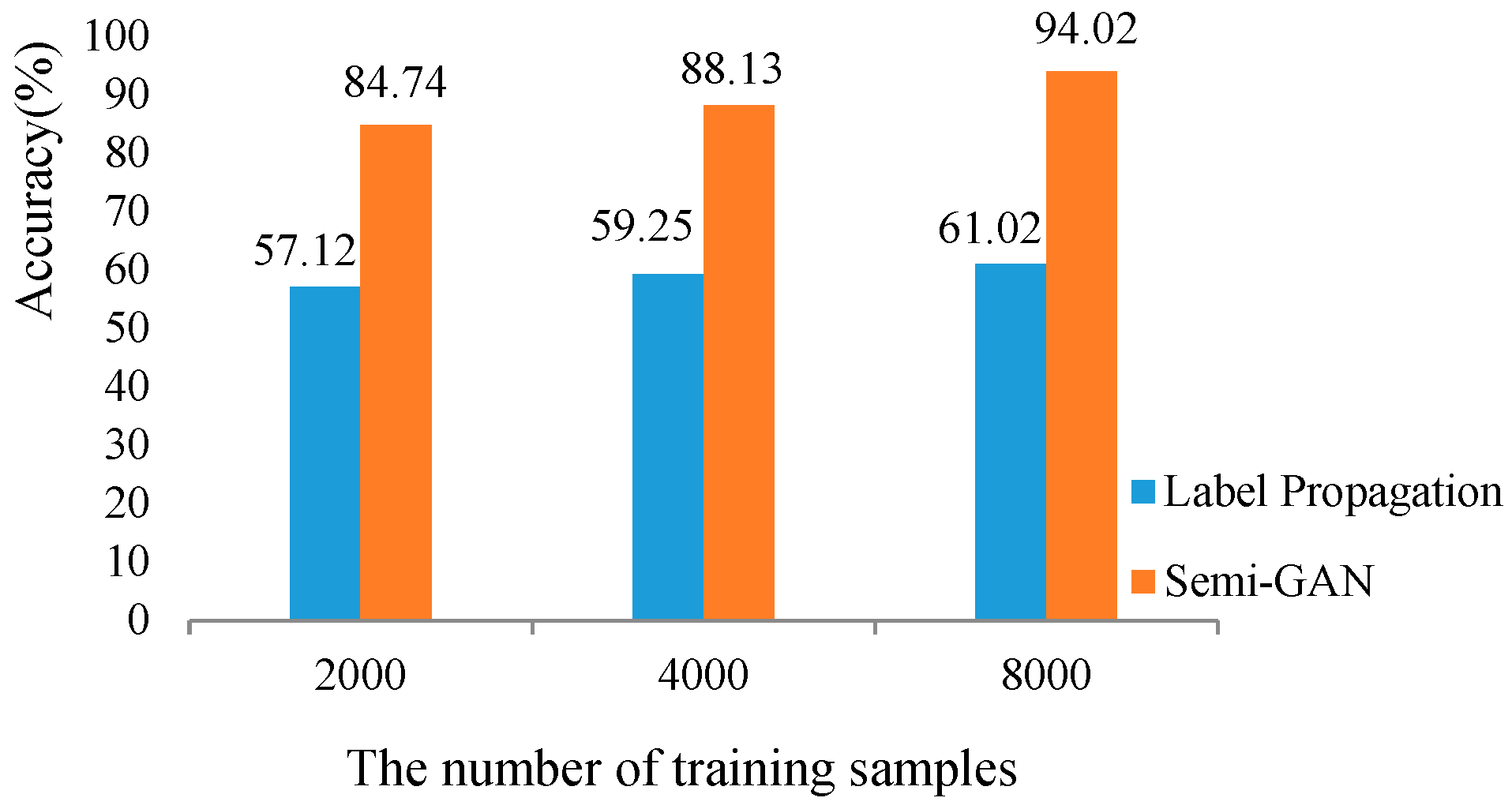
4.4. Limited Training Samples and Classification Maps

In this experiment, in order to make a comprehensive comparison between different supervised and semi-supervised methods, respectively, we calculated the results of OA when the number of training samples was changed. The results of supervised and semi-supervised methods were shown in Figure 6 and Figure 7, respectively.
For supervised methods, we chose the SVM, EMP-RF, and PCA-DenseNet to report the different capacities in coping with complex data when the number of training samples was reduced. For semi-supervised methods, the Label Propagation and Semi-GAN were chosen as the contrastive methods. Take the two figures apart, we can see that the PCA-DenseNet and Semi-GAN always obtained the highest OA in three different conditions for both supervised and semi-supervised classification. Compared with the traditional approaches used in HSI classification, the results demonstrated that the deep learning methods can exploit huge capacities in coping with complex data. When combining the two figures together, the Semi-GAN showed the best performance in all supervised and semi-supervised methods. Furthermore, we can see that the reduction of Semi-GAN was lower than PCA-DenseNet when the number of available training samples decreased, which proved that the semi-supervised methods obtained a superior ability than supervised approaches in the limited training samples condition.
Moreover, we visually analyzed the classification results. The investigated methods include SVM, EMP-RF, PCA-DenseNet, and Semi-GAN. The classification maps for different approaches were shown in Figure 8. From the maps, one can see how the different methods affected the classification results. The EMP-RF method had the lowest precise in the dataset (see Figure 8b), and compared with the traditional methods, the deep learning methods achieved a superior performance in classification, furthermore, we can see that our proposed Semi-GAN gave a more detailed classification map than PCA-DenseNet.

4.5. Consuming Time

In this study, the total running time for five repeated experiments of five methods, e.g., the CNN-based models and traditional SVM model, on this dataset were shown in Table 10. In the SVM method, we preserved three principal components of HSI after PCA, the 27 × 27 × 3 neighbors of each pixel were regarded as the input 3D image. In the CNN-based methods, the size of each input image was 64 × 64 × d, where the d represented the number of spectral bands in CNN and 64 × 64 × 10 in Semi-GAN and PCA-DenseNet. All the experiments were run on a 3.2-GHz CPU with a GTX 1060 GPU card. The CNN-based methods were performed on PyTorch platform and the SVM method was performed on LibSVM library.
From Table 10, one can see that SVM method had the longest running time. When coping with complicated data with large volume, the consuming time of SVM-based method increased sharply along with the increasing numbers of training samples, which made SVM not suitable for the classification with lots of training samples.
The deep models reduced the total consuming time drastically and improved the classification performance at the same time when compared with SVM model. Besides, the additional preprocessing operations like PCA and Auto-Encoder reduced the running time greatly, which make deep learning methods more applicable for the HSI fine-grained classification with a great number of classes.

5. Conclusions

The fine-grained classification of HSI is a task to be solved nowadays. In this study, deep learning-based methods were investigated for HSI supervised and semi-supervised fine-grained classification for the first time. The obtained experimental results have shown that the proposed deep learning-based methods obtained superior performance in terms of classification accuracy.
For supervised fine-grained classification of HSI, densely connected CNN was proposed for accurate classification. The deep learning-based methods significantly outperformed the traditional spectral-spatial classifiers such as SVM, EMP-RF, and EMAP-RF in terms of classification accuracy. Moreover, the combination of DenseNet with pre-processing or post-processing technique was proposed to further improve classification accuracy.
For semi-supervised fine-grained classification of HSI, GAN was used to handle the labeled and unlabeled samples in the training stage. The proposed 3D Semi-GAN achieved better classification performance compared with traditional semi-supervised classifiers such as TSVM and Label Propagation.
The proposed deep learning models worked effectively with different numbers of training samples. The deep models exhibited good classification performance (e.g., OA was 88.23%) even under limited training samples (e.g., 4000 training samples were available, which meant there were only 77 training samples for each class on average in Auto-Encoder-DenseNet). The study demonstrates that deep learning has a huge potential for HSI fine-grained classification.

Author Contributions

Conceptualization, Y.C.; methodology, L.H., L.Z., and Y.C.; writing—original draft preparation, Y.C., L.H., L.Z., N.Y., and X.J.

Funding

This research was funded by the Natural Science Foundation of China under the Grant 61971164.

Conflicts of Interest

The authors declare no conflict of interest.

References

  1. Fauvel, M.; Tarabalka, Y.; Benediktsson, J.A.; Chanussot, J.; Tilton, J.C. Advances in Spectral-Spatial Classification of Hyperspectral Images. Proc. IEEE 2012, 101, 652–675. [Google Scholar] [CrossRef]
  2. Chang, C.-I. Hyperspectral Imaging: Techniques for Spectral Detection and Classification; Kluwer Academic Publishers: New York, NY, USA, 2003; pp. 15–35. [Google Scholar]
  3. Li, J.; Bioucas-Dias, J.M.; Plaza, A. Spectral–spatial hyperspectral image segmentation using subspace multinomial logistic regression and Markov random fields. IEEE Trans. Geosci. Remote Sens. 2011, 50, 809–823. [Google Scholar] [CrossRef]
  4. Ham, J.; Chen, Y.; Crawford, M.M.; Ghosh, J. Investigation of the random forest framework for classification of hyperspectral data. IEEE Trans. Geosci. Remote Sens. 2005, 43, 492–501. [Google Scholar] [CrossRef]
  5. Yang, H. A back-propagation neural network for mineralogical mapping from AVIRIS data. Int. J. Remote Sens. 1999, 20, 97–110. [Google Scholar] [CrossRef]
  6. Gualtieri, J.A.; Cromp, R.F. Support vector machines for hyperspectral remote sensing classification. In Proceedings of the 27th AIPR Workshop: Advances in Computer-Assisted Recognition, Washington, DC, USA, 14–16 October 1998; pp. 221–232. [Google Scholar]
  7. Melgani, F.; Bruzzone, L. Classification of hyperspectral remote sensing images with support vector machines. IEEE Trans. Geosci. Remote Sens. 2004, 42, 1778–1790. [Google Scholar] [CrossRef]
  8. Chen, Y.; Nasrabadi, N.M.; Tran, T.D. Hyperspectral image classification using dictionary-based sparse representation. IEEE Trans. Geosci. Remote Sens. 2011, 49, 3973–3985. [Google Scholar] [CrossRef]
  9. Ghamisi, P.; Plaza, J.; Chen, Y.; Li, J.; Plaza, A.J. Advanced spectral classifiers for hyperspectral images: A review. IEEE Geosci. Remote Sens. Mag. 2017, 5, 8–32. [Google Scholar] [CrossRef]
  10. Xu, X.; Li, W.; Ran, Q.; Du, Q.; Gao, L.; Zhang, B. Multisource remote sensing data classification based on convolutional neural network. IEEE Trans. Geosci. Remote Sens. 2017, 56, 937–949. [Google Scholar] [CrossRef]
  11. Yang, X.; Ye, Y.; Li, X.; Lau, R.Y.; Zhang, X.; Huang, X. Hyperspectral image classification with deep learning models. IEEE Trans. Geosci. Remote Sens. 2018, 56, 5408–5423. [Google Scholar] [CrossRef]
  12. Chen, Y.; Zhao, X.; Jia, X. Spectral–spatial classification of hyperspectral data based on deep belief network. IEEE J. Sel. Top. Appl. Earth Obs. Remote Sens. 2015, 8, 2381–2392. [Google Scholar] [CrossRef]
  13. Palmason, J.A.; Benediktsson, J.A.; Sveinsson, J.R.; Chanussot, J. Classification of hyperspectral data from urban areas using morphological preprocessing and independent component analysis. In Proceedings of the 2005 IEEE International Geoscience and Remote Sensing Symposium, Seoul, Korea, 25–29 July 2005; pp. 176–179. [Google Scholar]
  14. Pesaresi, M.; Benediktsson, J.A. A new approach for the morphological segmentation of high-resolution satellite imagery. IEEE Trans. Geosci. Remote Sens. 2001, 39, 309–320. [Google Scholar] [CrossRef]
  15. Gu, Y.; Chanussot, J.; Jia, X.; Benediktsson, J.A. Multiple kernel learning for hyperspectral image classification: A review. IEEE Trans. Geosci. Remote Sens. 2017, 55, 6547–6565. [Google Scholar] [CrossRef]
  16. Fauvel, M.; Benediktsson, J.A.; Chanussot, J.; Sveinsson, J.R. Spectral and spatial classification of hyperspectral data using SVMs and morphological profiles. IEEE Trans. Geosci. Remote Sens. 2008, 46, 3804–3814. [Google Scholar] [CrossRef]
  17. Song, B.; Li, J.; Dalla Mura, M.; Li, P.; Plaza, A.; Bioucas-Dias, J.M.; Benediktsson, J.A.; Chanussot, J. Remotely sensed image classification using sparse representations of morphological attribute profiles. IEEE Trans. Geosci. Remote Sens. 2013, 52, 5122–5136. [Google Scholar] [CrossRef]
  18. Camps-Valls, G.; Gomez-Chova, L.; Muñoz-Marí, J.; Vila-Francés, J.; Calpe-Maravilla, J. Composite kernels for hyperspectral image classification. IEEE Geosci. Remote Sens. Lett. 2006, 3, 93–97. [Google Scholar] [CrossRef]
  19. Baraldi, A.; Bruzzone, L.; Blonda, P. Quality assessment of classification and cluster maps without ground truth knowledge. IEEE Trans. Geosci. Remote Sens. 2005, 43, 857–873. [Google Scholar] [CrossRef]
  20. Chi, M.; Bruzzone, L. A semilabeled-sample-driven bagging technique for ill-posed classification problems. IEEE Geosci. Remote Sens. Lett. 2005, 2, 69–73. [Google Scholar] [CrossRef]
  21. Shahshahani, B.M.; Landgrebe, D.A. The effect of unlabeled samples in reducing the small sample size problem and mitigating the Hughes phenomenon. IEEE Trans. Geosci. Remote Sens. 1994, 32, 1087–1095. [Google Scholar] [CrossRef]
  22. Bruzzone, L.; Chi, M.; Marconcini, M. A novel transductive SVM for semisupervised classification of remote-sensing images. IEEE Trans. Geosci. Remote Sens. 2006, 44, 3363–3373. [Google Scholar] [CrossRef]
  23. Camps-Valls, G.; Marsheva, T.V.B.; Zhou, D. Semi-supervised graph-based hyperspectral image classification. IEEE Trans. Geosci. Remote Sens. 2007, 45, 3044–3054. [Google Scholar] [CrossRef]
  24. Deng, J.; Dong, W.; Socher, R.; Li, L.-J.; Li, K.; Fei-Fei, L. Imagenet: A large-scale hierarchical image database. In Proceedings of the 2009 IEEE Conference on Computer Vision and Pattern Recognition, Miami, FL, USA, 20–25 June 2009; pp. 248–255. [Google Scholar]
  25. Hinton, G.; Deng, L.; Yu, D.; Dahl, G.; Mohamed, A.-r.; Jaitly, N.; Senior, A.; Vanhoucke, V.; Nguyen, P.; Kingsbury, B. Deep neural networks for acoustic modeling in speech recognition. IEEE Signal Process. Mag. 2012, 29, 82–97. [Google Scholar] [CrossRef]
  26. Gao, J.; He, X.; Yih, W.-T.; Deng, L. Learning semantic representations for the phrase translation model. arXiv 2013, arXiv:1312.0482. [Google Scholar]
  27. LeCun, Y.; Bengio, Y.; Hinton, G. Deep learning. Nature 2015, 521, 436. [Google Scholar] [CrossRef] [PubMed]
  28. Zhang, L.; Zhang, L.; Du, B. Deep learning for remote sensing data: A technical tutorial on the state of the art. IEEE Geosci. Remote Sens. Mag. 2016, 4, 22–40. [Google Scholar] [CrossRef]
  29. Chen, Y.; Lin, Z.; Zhao, X.; Wang, G.; Gu, Y. Deep learning-based classification of hyperspectral data. IEEE J. Sel. Top. Appl. Earth Obs. Remote Sens. 2014, 7, 2094–2107. [Google Scholar] [CrossRef]
  30. Ma, X.; Wang, H.; Geng, J. Spectral–spatial classification of hyperspectral image based on deep auto-encoder. IEEE J. Sel. Top. Appl. Earth Obs. Remote Sens. 2016, 9, 4073–4085. [Google Scholar] [CrossRef]
  31. Zhong, P.; Gong, Z.; Li, S.; Schönlieb, C.-B. Learning to diversify deep belief networks for hyperspectral image classification. IEEE Trans. Geosci. Remote Sens. 2017, 55, 3516–3530. [Google Scholar] [CrossRef]
  32. Chen, Y.; Jiang, H.; Li, C.; Jia, X.; Ghamisi, P. Deep feature extraction and classification of hyperspectral images based on convolutional neural networks. IEEE Trans. Geosci. Remote Sens. 2016, 54, 6232–6251. [Google Scholar] [CrossRef]
  33. Hu, W.; Huang, Y.; Wei, L.; Zhang, F.; Li, H. Deep convolutional neural networks for hyperspectral image classification. J. Sens. 2015, 1–12. [Google Scholar] [CrossRef]
  34. Romero, A.; Gatta, C.; Camps-Valls, G. Unsupervised deep feature extraction for remote sensing image classification. IEEE Trans. Geosci. Remote Sens. 2015, 54, 1349–1362. [Google Scholar] [CrossRef]
  35. Tao, Y.; Xu, M.; Lu, Z.; Zhong, Y. DenseNet-based depth-width double reinforced deep learning neural network for high-resolution remote sensing image per-pixel classification. Remote Sens. 2018, 10, 779. [Google Scholar] [CrossRef]
  36. Mou, L.; Ghamisi, P.; Zhu, X.X. Deep recurrent neural networks for hyperspectral image classification. IEEE Trans. Geosci. Remote Sens. 2017, 55, 3639–3655. [Google Scholar] [CrossRef] [Green Version]
  37. Zhao, W.; Du, S. Spectral–spatial feature extraction for hyperspectral image classification: A dimension reduction and deep learning approach. IEEE Trans. Geosci. Remote Sens. 2016, 54, 4544–4554. [Google Scholar] [CrossRef]
  38. Li, W.; Wu, G.; Zhang, F.; Du, Q. Hyperspectral image classification using deep pixel-pair features. IEEE Trans. Geosci. Remote Sens. 2016, 55, 844–853. [Google Scholar] [CrossRef]
  39. Zhong, Z.; Li, J.; Luo, Z.; Chapman, M. Spectral–spatial residual network for hyperspectral image classification: A 3-D deep learning framework. IEEE Trans. Geosci. Remote Sens. 2017, 56, 847–858. [Google Scholar] [CrossRef]
  40. Li, Y.; Zhang, H.; Shen, Q. Spectral–spatial classification of hyperspectral imagery with 3D convolutional neural network. Remote Sens. 2017, 9, 67. [Google Scholar] [CrossRef] [Green Version]
  41. Sellami, A.; Farah, M.; Farah, I.R.; Solaiman, B. Hyperspectral imagery classification based on semi-supervised 3-D deep neural network and adaptive band selection. Expert Syst. Appl. 2019, 129, 246–259. [Google Scholar] [CrossRef]
  42. Zhu, L.; Chen, Y.; Ghamisi, P.; Benediktsson, J.A. Generative adversarial networks for hyperspectral image classification. IEEE Trans. Geosci. Remote Sens. 2018, 56, 5046–5063. [Google Scholar] [CrossRef]
  43. Zhan, Y.; Hu, D.; Wang, Y.; Yu, X. Semisupervised hyperspectral image classification based on generative adversarial networks. IEEE Geosci. Remote Sens. Lett. 2017, 15, 212–216. [Google Scholar] [CrossRef]
  44. Cavallaro, G.; Riedel, M.; Richerzhagen, M.; Benediktsson, J.A.; Plaza, A. On understanding big data impacts in remotely sensed image classification using support vector machine methods. IEEE J. Sel. Top. Appl. Earth Obs. Remote Sens. 2015, 8, 4634–4646. [Google Scholar] [CrossRef] [Green Version]
  45. Richards, J.A.; Richards, J. Remote Sensing Digital Image Analysis; Springer: Berlin, Germany, 1999; pp. 161–201. [Google Scholar]
  46. Mughees, A.; Tao, L. Efficient deep auto-encoder learning for the classification of hyperspectral images. In Proceedings of the 2016 International Conference on Virtual Reality and Visualization (ICVRV), Hangzhou, China, 23–25 September 2016; pp. 44–51. [Google Scholar]
  47. Chu, X.; Ouyang, W.; Wang, X. Crf-cnn: Modeling structured information in human pose estimation. In Proceedings of the Advances in Neural Information Processing Systems, Barcelona, Spain, 5–10 December 2016; pp. 316–324. [Google Scholar]
  48. Kirillov, A.; Schlesinger, D.; Zheng, S.; Savchynskyy, B.; Torr, P.H.; Rother, C. Joint training of generic CNN-CRF models with stochastic optimization. In Proceedings of the Asian Conference on Computer Vision, Taipei, China, 20–24 November 2016; pp. 221–236. [Google Scholar]
  49. Liu, F.; Lin, G.; Shen, C. CRF learning with CNN features for image segmentation. Pattern Recognit. 2015, 48, 2983–2992. [Google Scholar] [CrossRef] [Green Version]
  50. Chen, L.-C.; Papandreou, G.; Kokkinos, I.; Murphy, K.; Yuille, A.L. Semantic image segmentation with deep convolutional nets and fully connected crfs. arXiv 2014, arXiv:1412.7062. [Google Scholar]
  51. Zheng, S.; Jayasumana, S.; Romera-Paredes, B.; Vineet, V.; Su, Z.; Du, D.; Huang, C.; Torr, P.H. Conditional random fields as recurrent neural networks. In Proceedings of the IEEE International Conference on Computer Vision, Santiago, Chile, 13–16 December 2015; pp. 1529–1537. [Google Scholar]
  52. Ioffe, S.; Szegedy, C. Batch normalization: Accelerating deep network training by reducing internal covariate shift. arXiv 2015, arXiv:1502.03167. [Google Scholar]
  53. Santurkar, S.; Tsipras, D.; Ilyas, A.; Madry, A. How does batch normalization help optimization? In Proceedings of the Advances in Neural Information Processing Systems, Montreal, QC, Canada, 2–8 December 2018; pp. 2483–2493. [Google Scholar]
  54. Huang, G.; Liu, Z.; Van Der Maaten, L.; Weinberger, K.Q. Densely connected convolutional networks. In Proceedings of the IEEE Conference on Computer Vision and Pattern Recognition, Honolulu, HI, USA, 21–26 July 2017; pp. 4700–4708. [Google Scholar]
  55. Rother, C.; Kolmogorov, V.; Blake, A. Grabcut: Interactive foreground extraction using iterated graph cuts. ACM Trans. Gr. (TOG) 2004, 23, 309–314. [Google Scholar] [CrossRef]
  56. Shotton, J.; Winn, J.; Rother, C.; Criminisi, A. Textonboost for image understanding: Multi-class object recognition and segmentation by jointly modeling texture, layout, and context. Int. J. Comput. Vision 2009, 81, 2–23. [Google Scholar] [CrossRef] [Green Version]
  57. Krähenbühl, P.; Koltun, V. Efficient inference in fully connected crfs with gaussian edge potentials. In Proceedings of the Advances in Neural Information Processing Systems, Granada, Spain, 12–17 December 2011; pp. 109–117. [Google Scholar]
  58. Goodfellow, I.; Pouget-Abadie, J.; Mirza, M.; Xu, B.; Warde-Farley, D.; Ozair, S.; Courville, A.; Bengio, Y. Generative adversarial nets. In Proceedings of the Advances in Neural Information Processing Systems, Montreal, QC, Canada, 8–13 December 2014; pp. 2672–2680. [Google Scholar]
  59. Mirza, M.; Osindero, S. Conditional generative adversarial nets. arXiv 2014, arXiv:1411.1784. [Google Scholar]
  60. Ledig, C.; Theis, L.; Huszár, F.; Caballero, J.; Cunningham, A.; Acosta, A.; Aitken, A.; Tejani, A.; Totz, J.; Wang, Z. Photo-realistic single image super-resolution using a generative adversarial network. In Proceedings of the 2009 IEEE Conference on Computer Vision and Pattern Recognition, Miami, FL, USA, 20–25 June 2009; pp. 4681–4690. [Google Scholar]
  61. Zhu, J.-Y.; Park, T.; Isola, P.; Efros, A.A. Unpaired image-to-image translation using cycle-consistent adversarial networks. In Proceedings of the IEEE International Conference on Computer Vision, Venice, Italy, 22–29 October 2017; pp. 2223–2232. [Google Scholar]
  62. Yi, Z.; Zhang, H.; Tan, P.; Gong, M. Dualgan: Unsupervised dual learning for image-to-image translation. In Proceedings of the IEEE International Conference on Computer Vision, Venice, Italy, 22–29 October 2017; pp. 2849–2857. [Google Scholar]
  63. Mathieu, M.; Couprie, C.; LeCun, Y. Deep multi-scale video prediction beyond mean square error. arXiv 2015, arXiv:1511.05440. [Google Scholar]
  64. Li, C.; Wand, M. Precomputed real-time texture synthesis with markovian generative adversarial networks. In Proceedings of the European Conference on Computer Vision, Amsterdam, The Netherlands, 8–16 October 2016; pp. 702–716. [Google Scholar]
  65. Yu, L.; Zhang, W.; Wang, J.; Yu, Y. Seqgan: Sequence generative adversarial nets with policy gradient. In Proceedings of the Thirty-First AAAI Conference on Artificial Intelligence, San Francisco, CA, USA, 4–9 February 2017. [Google Scholar]
  66. Radford, A.; Metz, L.; Chintala, S. Unsupervised representation learning with deep convolutional generative adversarial networks. arXiv 2015, arXiv:1511.06434. [Google Scholar]
  67. Arjovsky, M.; Chintala, S.; Bottou, L. Wasserstein gan. arXiv 2017, arXiv:1701.07875. [Google Scholar]
  68. Odena, A.; Olah, C.; Shlens, J. Conditional image synthesis with auxiliary classifier gans. In Proceedings of the 34th International Conference on Machine Learning, Sydney, Australia, 6–11 August 2017; Volume 70, pp. 2642–2651. [Google Scholar]
  69. Chang, C.-C.; Lin, C.-J. LIBSVM: A library for support vector machines. ACM Trans. Intell. Syst. Technol. 2011, 2, 27. [Google Scholar] [CrossRef]
  70. Breiman, L. RF/tools: A class of two-eyed algorithms. In Proceedings of the SIAM Workshop, San Francisco, CA, USA, 1–3 May 2003; pp. 1–56. [Google Scholar]
  71. Dalla Mura, M.; Atli Benediktsson, J.; Waske, B.; Bruzzone, L. Extended profiles with morphological attribute filters for the analysis of hyperspectral data. Int. J. Remote Sens. 2010, 31, 5975–5991. [Google Scholar] [CrossRef]
  72. Dalla Mura, M.; Benediktsson, J.A.; Waske, B.; Bruzzone, L. Morphological attribute profiles for the analysis of very high resolution images. IEEE Trans. Geosci. Remote Sens. 2010, 48, 3747–3762. [Google Scholar] [CrossRef]
  73. Ghamisi, P.; Benediktsson, J.A.; Cavallaro, G.; Plaza, A. Automatic framework for spectral–spatial classification based on supervised feature extraction and morphological attribute profiles. IEEE J. Sel. Top. Appl. Earth Obs. Remote Sens. 2014, 7, 2147–2160. [Google Scholar] [CrossRef]
  74. Salimans, T.; Goodfellow, I.; Zaremba, W.; Cheung, V.; Radford, A.; Chen, X. Improved techniques for training gans. In Proceedings of the Advances in Neural Information Processing Systems, Barcelona, Spain, 5–10 December 2016; pp. 2234–2242. [Google Scholar]
Figure 1. The framework of DenseNet for HSI supervised fine-grained classification.
Remotesensing 11 02690 g001
Figure 2. A four-layer dense block.
Remotesensing 11 02690 g002
Figure 3. The framework of HSI semi-supervised fine-grained classification.
Remotesensing 11 02690 g003
Figure 4. The Indian Pines dataset. (a) False-color composite image (Band 40, 25, 10); (b) ground reference map.
Remotesensing 11 02690 g004
Figure 5. Test accuracy of different supervised methods on the Indian Pines dataset.
Remotesensing 11 02690 g005
Figure 6. Test accuracy of different supervised methods with changed number of training samples.
Remotesensing 11 02690 g006
Figure 7. Test accuracy of different semi-supervised methods with changed number of training samples.
Remotesensing 11 02690 g007
Figure 8. (a) False-color composite image of Indian Pines dataset; The classification maps using (b) EMP-RF; (c) PCA-DenseNet; (d) DenseNet-CRF; (e) Semi-GAN.
Remotesensing 11 02690 g008
Table 1. The distribution of the 52 classes.
No.ColorNumber of SamplesNumber of Training Samples (I)Number of Training Samples (II)Number of Test Samples (I)Number of Test Samples (II)
1 Remotesensing 11 02690 i00117,19542343610801042
2 Remotesensing 11 02690 i00217,78342843710431088
3 Remotesensing 11 02690 i00315834611
4 Remotesensing 11 02690 i0045141094132
5 Remotesensing 11 02690 i00523565368130139
6 Remotesensing 11 02690 i00612,404319300677732
7 Remotesensing 11 02690 i00726,48663861216001556
8 Remotesensing 11 02690 i00839,67898594724712400
9 Remotesensing 11 02690 i00980012164747
10 Remotesensing 11 02690 i01017283640105127
11 Remotesensing 11 02690 i011104929315463
12 Remotesensing 11 02690 i0125629144149318311
13 Remotesensing 11 02690 i0138862204205550541
14 Remotesensing 11 02690 i0144381114109240249
15 Remotesensing 11 02690 i015120636437780
16 Remotesensing 11 02690 i0165685131125358367
17 Remotesensing 11 02690 i01711462104
18 Remotesensing 11 02690 i018114729275678
19 Remotesensing 11 02690 i01923315171132148
20 Remotesensing 11 02690 i020112830255361
21 Remotesensing 11 02690 i02121854953124138
22 Remotesensing 11 02690 i02222585251144140
23 Remotesensing 11 02690 i02322457813
24 Remotesensing 11 02690 i02419405038116124
25 Remotesensing 11 02690 i02517424253103106
26 Remotesensing 11 02690 i0263357101418
27 Remotesensing 11 02690 i02710,386273210634657
28 Remotesensing 11 02690 i0281024268
29 Remotesensing 11 02690 i0299391220223553597
30 Remotesensing 11 02690 i03089423225145
31 Remotesensing 11 02690 i031111023267475
32 Remotesensing 11 02690 i0325074109138293318
33 Remotesensing 11 02690 i03327264561159166
34 Remotesensing 11 02690 i03411,802249266677707
35 Remotesensing 11 02690 i03510,387247253660608
36 Remotesensing 11 02690 i03622426440115126
37 Remotesensing 11 02690 i0375432062823
38 Remotesensing 11 02690 i03815,118339382904885
39 Remotesensing 11 02690 i03926674963166159
40 Remotesensing 11 02690 i04018325154122107
41 Remotesensing 11 02690 i0418098188186460484
42 Remotesensing 11 02690 i0424953128140281295
43 Remotesensing 11 02690 i04321574155133137
44 Remotesensing 11 02690 i04425333956120158
45 Remotesensing 11 02690 i04592926284955
46 Remotesensing 11 02690 i0468731221215535498
47 Remotesensing 11 02690 i04758311163630
48 Remotesensing 11 02690 i04831109269190194
49 Remotesensing 11 02690 i04958012143936
50 Remotesensing 11 02690 i0504979118118281293
51 Remotesensing 11 02690 i05163,5621519148638613715
52 Remotesensing 11 02690 i05214433169
Total number333,9518000800020,00020,000
Table 2. The detailed framework of DenseNet.
LayersOutput SizeDenseNet
Convolution56 × 569 × 9 conv, stride = 1
Dense Block
(1)
56 × 56 ( 1 × 1   conv 3 × 3   conv ) × 2
Transition Layer
(1)
56 × 561 × 1 conv
28 × 282 × 2 average pool, stride = 2
Dense Block
(2)
28 × 28 ( 1 × 1   conv 3 × 3   conv ) × 4
Transition Layer
(2)
28 × 281 × 1 conv
14 × 142 × 2 average pool, stride = 2
Dense Block
(3)
14 × 14 ( 1 × 1   conv 3 × 3   conv ) × 6
Transition Layer
(3)
14 × 141 × 1 conv
7 × 72 × 2 average pool, stride = 2
Dense Block
(4)
7 × 7 ( 1 × 1   conv 3 × 3   conv ) × 8
Classification Layer1 × 17 × 7 global average pool
fully-connected, softmax
Table 3. Test accuracy of Auto-Encoder-DenseNet with different numbers of principal components.
Number of Principal Components51020
OA (%)91.48 ± 0.4292.35 ± 0.5792.23 ± 0.53
AA (%)86.54 ± 1.7687.89 ± 2.0787.44 ± 1.65
K × 10089.61 ± 0.5491.30 ± 0.6691.12 ± 0.79
Table 4. The detailed parameter settings of deep models.
ModelLearning RateNumber of EpochsBatch Size
Auto-Encoder0.0011505000
CNN0.001150200
DenseNet0.001150200
Semi-GAN0.0002200200
Table 5. Test accuracy with different supervised methods on the Indian Pines dataset.
NoColorSVMEMP-RFEMAP-RFCNNCNN-CRFPCA-DenseNetAuto-Encoder-DenseNetDenseNet-CRF
1 Remotesensing 11 02690 i00152.61 ± 4.3569.71 ± 3.2460.09 ± 3.2477.77 ± 2.0185.54 ± 1.1784.45 ± 0.4984.93 ± 2.7490.92 ± 0.02
2 Remotesensing 11 02690 i00232.68 ± 6.3471.96 ± 5.6966.84 ± 5.6971.40 ± 4.5685.08 ± 2.4394.59 ± 0.8289.44 ± 1.7889.96 ± 0.26
3 Remotesensing 11 02690 i00318.142 ± 6.1228.43 ± 0.3823.05 ± 0.1672.72 ± 0.0480.22 ± 0.5087.22 ± 9.2481.11 ± 2.5486.67 ± 0.15
4 Remotesensing 11 02690 i00417.00 ± 9.2220.26 ± 5.1249.05 ± 5.1286.06 ± 5.3572.05 ± 3.4587.53 ± 3.5476.86 ± 3.8791.47 ± 0.19
5 Remotesensing 11 02690 i00518.91 ± 5.3260.81 ± 5.7667.48 ± 6.3488.39 ± 1.9383.61 ± 0.1290.37 ± 1.9494.13 ± 4.3391.41 ± 0.05
6 Remotesensing 11 02690 i00628.30 ± 0.0367.44 ± 4.3578.24 ± 4.5682.33 ± 0.4584.90 ± 0.0893.08 ± 0.2190.26 ± 3.6090.79 ± 0.07
7 Remotesensing 11 02690 i00733.86 ± 2.1575.58 ± 0.3472.65 ± 0.0877.46 ± 2.5580.06 ± 1.4593.07 ± 0.2594.41 ± 3.0592.67 ± 0.43
8 Remotesensing 11 02690 i00834.25 ± 0.0382.49 ± 1.0485.05 ± 0.1684.84 ± 1.4584.87 ± 0.0595.82 ± 0.3594.68 ± 2.2493.23 ± 0.21
9 Remotesensing 11 02690 i0099.56 ± 2.5466.34 ± 3.0259.15 ± 2.2487.36 ± 4.4597.45 ± 0.46100.00 ± 0.00100.00 ± 0.0096.97 ± 0.19
10 Remotesensing 11 02690 i01016.10 ± 0.0344.74 ± 8.4368.45 ± 3.4680.82 ± 5.3490.90 ± 2.4596.37 ± 1.4896.18 ± 1.4590.47 ± 0.03
11 Remotesensing 11 02690 i01119.77 ± 0.1342.31 ± 1.1676.37 ± 2.0872.11 ± 0.1789.77 ± 2.5687.78 ± 2.4681.26 ± 3.6587.02 ± 0.09
12 Remotesensing 11 02690 i01227.30 ± 6.4565.46 ± 5.0276.15 ± 4.3575.91 ± 3.4589.94 ± 1.5695.05 ± 0.7192.90 ± 3.1093.38 ± 0.16
13 Remotesensing 11 02690 i01337.87 ± 5.6374.57 ± 4.5381.86 ± 0.0386.37 ± 3.5691.46 ± 4.3293.58 ± 0.9194.63 ± 2.7090.93 ± 0.15
14 Remotesensing 11 02690 i01436.31 ± 9.4668.15 ± 3.4681.58 ± 3.1380.96 ± 0.0886.49 ± 0.1291.52 ± 0.2488.32 ± 3.9292.03 ± 0.23
15 Remotesensing 11 02690 i01535.84 ± 1.9858.33 ± 3.4566.70 ± 0.2177.63 ± 2.4689.23 ± 1.5690.91 ± 0.4596.36 ± 2.5396.42 ± 0.15
16 Remotesensing 11 02690 i01657.14 ± 2.5470.01 ± 0.4285.65 ± 0.1481.69 ± 0.4383.57 ± 0.2093.97 ± 0.9696.97 ± 1.2494.54 ± 0.06
17 Remotesensing 11 02690 i01739.25 ± 12.5355.56 ± 9.4343.25 ± 0.1573.33 ± 9.3065.42 ± 0.143.82 ± 5.2576.61 ± 2.1491.37 ± 0.42
18 Remotesensing 11 02690 i01823.19 ± 9.0725.39 ± 7.4534.78 ± 0.2547.61 ± 0.1578.72 ± 0.1565.71 ± 5.8169.27 ± 3.7380.51 ± 0.32
19 Remotesensing 11 02690 i01952.65 ± 7.5366.62 ± 6.2678.95 ± 2.4385.81 ± 2.4585.87 ± 3.5687.67 ± 1.5591.17 ± 2.9691.28 ± 0.06
20 Remotesensing 11 02690 i02048.63 ± 7.1557.06 ± 4.5655.58 ± 3.2373.91 ± 3.4590.47 ± 3.4671.20 ± 3.9692.23 ± 1.2486.74 ± 0.04
21 Remotesensing 11 02690 i02163.14 ± 0.0669.24 ± 0.1482.85 ± 0.0262.48 ± 0.2179.62 ± 2.3590.01 ± 1.8795.50 ± 2.3792.83 ± 0.12
22 Remotesensing 11 02690 i02268.35 ± 2.8968.14 ± 1.3583.25 ± 2.3970.94 ± 0.9879.36 ± 0.2490.98 ± 1.5591.07 ± 3.1089.86 ± 0.14
23 Remotesensing 11 02690 i02361.51 ± 0.2483.33 ± 0.1672.57 ± 0.0392.85 ± 0.0189.18 ± 0.4679.36 ± 3.1928.34 ± 2.45100.00 ± 0.000
24 Remotesensing 11 02690 i02439.94 ± 1.5451.69 ± 0.6871.34 ± 0.3565.74 ± 0.1589.20 ± 0.2371.77 ± 3.6479.79 ± 0.0186.88 ± 0.16
25 Remotesensing 11 02690 i02544.63 ± 7.5458.35 ± 5.4563.02 ± 5.0176.54 ± 2.4582.74 ± 0.3477.45 ± 7.2269.13 ± 2.5675.67 ± 0.24
26 Remotesensing 11 02690 i02633.24 ± 0.0514.14 ± 0.0437.35 ± 0.1335.05 ± 0.2572.35 ± 0.1658.40 ± 9.3754.13 ± 2.7281.76 ± 0.32
27 Remotesensing 11 02690 i02765.98 ± 4.3376.01 ± 2.4583.55 ± 3.0990.36 ± 3.0178.37 ± 0.2691.13 ± 0.8991.46 ± 1.5091.92 ± 0.04
28 Remotesensing 11 02690 i02828.33 ± 0.1425.22 ± 4.6423.79 ± 13.5420.49 ± 10.2426.25 ± 0.1970.83 ± 1.3170.79 ± 3.1887.78 ± 0.42
29 Remotesensing 11 02690 i02943.25 ± 3.4669.28 ± 10.4576.58 ± 0.1973.01 ± 0.8787.90 ± 1.5689.48 ± 0.3690.51 ± 1.0790.73 ± 0.13
30 Remotesensing 11 02690 i03016.56 ± 2.0662.32 ± 0.1169.36 ± 0.0446.69 ± 2.5686.06 ± 0.1290.44 ± 0.9792.20 ± 0.1394.12 ± 0.04
31 Remotesensing 11 02690 i03115.54 ± 6.7470.62 ± 5.3962.95 ± 6.4389.41 ± 4.6749.29 ± 1.4584.97 ± 2.5986.90 ± 1.0891.91 ± 0.20
32 Remotesensing 11 02690 i03229.97 ± 7.4657.49 ± 6.3466.75 ± 4.6779.16 ± 0.3690.12 ± 2.4590.47 ± 0.1492.92 ± 0.4590.82 ± 0.05
33 Remotesensing 11 02690 i03323.64 ± 6.4268.59 ± 4.0777.39 ± 1.5691.51 ± 4.5782.71 ± 0.2590.52 ± 2.5989.55 ± 2.8588.65 ± 0.06
34 Remotesensing 11 02690 i03435.00 ± 4.5674.15 ± 8.3176.85 ± 6.4682.73 ± 5.6786.54 ± 0.4392.01 ± 0.1491.24 ± 1.2790.90 ± 0.23
35 Remotesensing 11 02690 i03524.83 ± 5.0368.78 ± 4.0472.75 ± 6.2387.37 ± 4.9282.82 ± 0.5195.29 ± 0.5295.35 ± 0.1591.35 ± 0.11
36 Remotesensing 11 02690 i03647.15 ± 0.0553.33 ± 0.0674.55 ± 0.1491.26 ± 0.4586.71 ± 1.5694.15 ± 1.8085.65 ± 0.0796.63 ± 0.39
37 Remotesensing 11 02690 i03726.99 ± 5.4354.77 ± 4.5651.45 ± 6.4381.42 ± 1.4590.20 ± 0.3292.47 ± 0.0294.01 ± 0.0498.96 ± 0.06
38 Remotesensing 11 02690 i03840.86 ± 6.4272.75 ± 3.6469.75 ± 2.3474.94 ± 2.4589.96 ± 0.1290.70 ± 0.4992.95 ± 0.0186.10 ± 0.24
39 Remotesensing 11 02690 i03954.55 ± 4.5668.54 ± 2.5461.24 ± 2.4588.53 ± 1.4673.64 ± 1.5790.18 ± 0.3791.61 ± 2.6489.91 ± 0.08
40 Remotesensing 11 02690 i04050.53 ± 2.0370.01 ± 0.7462.99 ± 3.4586.42 ± 1.9082.37 ± 0.3194.70 ± 1.6397.26 ± 3.1485.82 ± 0.25
41 Remotesensing 11 02690 i04149.15 ± 6.6471.46 ± 3.4586.25 ± 0.1389.72 ± 3.5782.24 ± 0.3496.32 ± 0.9494.33 ± 0.1390.99 ± 0.06
42 Remotesensing 11 02690 i04231.88 ± 4.4365.17 ± 2.1578.95 ± 1.4584.82 ± 0.0384.94 ± 0,5697.46 ± 0.3795.84 ± 3.2591.01 ± 0.05
43 Remotesensing 11 02690 i04343.98 ± 9.4665.55 ± 5.6478.84 ± 0.0985.49 ± 4.6782.36 ± 0.4586.02 ± 0.8192.61 ± 2.1494.90 ± 0.12
44 Remotesensing 11 02690 i04441.55 ± 3.5682.38 ± 0.0460.65 ± 0.0685.12 ± 2.5491.44 ± 0.1088.62 ± 1.8396.16 ± 2.0697.78 ± 0.10
45 Remotesensing 11 02690 i04547.40 ± 3.6459.18 ± 0.0481.02 ± 3.4272.66 ± 1.3679.33 ± 0.4269.66 ± 6.4588.13 ± 1.0278.03 ± 0.51
46 Remotesensing 11 02690 i04661.53 ± 0.0471.59 ± 0.5687.55 ± 3.4689.08 ± 0.6782.66 ± 0.3292.61 ± 0.2691.35 ± 0.4593.51 ± 0.05
47 Remotesensing 11 02690 i04761.05 ± 1.9740.18 ± 0.0485.35 ± 0.3286.04 ± 0.1481.18 ± 0.2494.75 ± 1.5179.89 ± 4.8891.30 ± 0.24
48 Remotesensing 11 02690 i04869.26 ± 4.5699.49 ± 3.5381.97 ± 0.3695.06 ± 2.5688.41 ± 0.4296.40 ± 1.1998.26 ± 0.8895.08 ± 0.04
49 Remotesensing 11 02690 i04953.92 ± 0.1479.82 ± 0.0879.76 ± 0.5778.37 ± 0.1784.47 ± 3.4679.32 ± 4.19100.00 ± 0.0095.99 ± 0.22
50 Remotesensing 11 02690 i05078.48 ± 4.5682.81 ± 4.3465.86 ± 2.4492.16 ± 2.4583.47 ± 2.4590.40 ± 2.4993.02 ± 0.5291.70 ± 0.34
51 Remotesensing 11 02690 i05172.48 ± 4.6496.95 ± 1.4581.44 ± 0.9796.26 ± 1.4584.45 ± 0.4697.96 ± 0.1997.35 ± 0.2196.58 ± 0.10
52 Remotesensing 11 02690 i05283.28 ± 1.4561.71 ± 3.4543.25 ± 0.6877.50 ± 0.1485.01 ± 0.21100.00 ± 0.0079.58 ± 3.4391.67 ± 0.12
OA (%)52.24 ± 0.4376.36 ± 0.2477.95 ± 0.5785.47 ± 0.2886.08 ± 0.2192.08 ± 0.8792.35 ± 0.5793.07 ± 0.18
AA (%)42.55 ± 0.1664.79 ± 0.3966.05 ± 0.1278.29 ± 0.2382.53 ± 0.8687.01 ± 1.2587.89 ± 2.0791.45 ± 0.31
K × 10047.15 ± 0.2072.24 ± 0.3573.72 ± 0.6682.86 ± 0.1385.64 ± 0.2790.26 ± 0.9491.30 ± 0.6692.76 ± 0.19
Table 6. Test accuracy with different preprocessing methods on the Indian Pines dataset.
NO.ColorCNNPCA-CNNAuto-Encoder-CNNDenseNetPCA-DenseNetDenseNet-1 × 1 ConvAuto-Encoder-DenseNet
1 Remotesensing 11 02690 i00177.77 ± 2.0177.69 ± 1.0986.18 ± 0.4583.32 ± 1.2584.45 ± 0.4982.45 ± 1.5984.93 ± 2.74
2 Remotesensing 11 02690 i00271.40 ± 4.5684.91 ± 0.4277.87 ± 0.7893.16 ± 0.4394.59 ± 0.8293.28 ± 1.2689.44 ± 1.78
3 Remotesensing 11 02690 i00372.72 ± 0.0472.40 ± 7.0994.56 ± 0.2368.58 ± 15.1487.22 ± 9.2466.59 ± 2.1581.11 ± 2.54
4 Remotesensing 11 02690 i00486.06 ± 5.3590.87 ± 5.1980.57 ± 2.5367.79 ± 5.8287.53 ± 3.5475.86 ± 3.1976.86 ± 3.87
5 Remotesensing 11 02690 i00588.39 ± 1.9394.02 ± 0.1578.33 ± 0.6688.62 ± 1.3990.37 ± 1.9481.19 ± 2.1594.13 ± 4.33
6 Remotesensing 11 02690 i00682.33 ± 0.4585.16 ± 0.6085.61 ± 0.6091.65 ± 2.0593.08 ± 0.2192.45 ± 0.4390.26 ± 3.60
7 Remotesensing 11 02690 i00777.46 ± 2.5589.57 ± 1.1287.82 ± 0.16 93.63 ± 0.4393.07 ± 0.2593.79 ± 0.2194.41 ± 3.05
8 Remotesensing 11 02690 i00884.84 ± 1.4593.75 ± 0.6694.47 ± 0.6695.61 ± 0.4295.82 ± 0.3595.69 ± 0.1994.68 ± 2.24
9 Remotesensing 11 02690 i00987.36 ± 4.45100.00 ± 0.0091.00 ± 0.1296.98 ± 1.69100.00 ± 0.0096.46 ± 1.68100.00 ± 0.00
10 Remotesensing 11 02690 i01080.82 ± 5.3495.11 ± 2.2593.11 ± 0.7995.79 ± 0.8996.37 ± 1.4890.36 ± 0.0996.18 ± 1.45
11 Remotesensing 11 02690 i01172.11 ± 0.1775.95 ± 1.2590.76 ± 1.2594.58 ± 0.8087.78 ± 2.4688.04 ± 0.1681.26 ± 3.65
12 Remotesensing 11 02690 i01275.91 ± 3.4585.67 ± 1.5488.00 ± 0.7693.59 ± 0.7295.05 ± 0.7193.18 ± 0.1592.90 ± 3.10
13 Remotesensing 11 02690 i01386.37 ± 3.5694.41 ± 0.7394.46 ± 0.1197.06 ± 0.3293.58 ± 0.9192.43 ± 0.2394.63 ± 2.70
14 Remotesensing 11 02690 i01480.96 ± 0.0888.89 ± 1.5691.69 ± 0.0288.36 ± 1.5091.52 ± 0.2494.73 ± 0.1588.32 ± 3.92
15 Remotesensing 11 02690 i01577.63 ± 2.4695.19 ± 1.4498.58 ± 0.0285.33 ± 2.1190.91 ± 0.4596.47 ± 3.5896.41 ± 2.53
16 Remotesensing 11 02690 i01681.69 ± 0.4398.49 ± 0.3897.11 ± 0.6996.71 ± 0.6893.97 ± 0.9695.96 ± 0.4296.97 ± 1.24
17 Remotesensing 11 02690 i01773.33 ± 9.3060.02 ± 13.9440.00 ± 13.3432.75 ± 10.253.82 ± 5.2598.67 ± 0.3276.61 ± 2.14
18 Remotesensing 11 02690 i01847.61 ± 0.1563.06 ± 2.5164.76 ± 2.5471.55 ± 6.2765.71 ± 5.8175.26 ± 4.2369.27 ± 3.73
19 Remotesensing 11 02690 i01985.81 ± 2.4593.22 ± 1.6172.99 ± 2.0383.52 ± 1.9787.67 ± 1.5594.18 ± 2.4191.28 ± 2.96
20 Remotesensing 11 02690 i02073.91 ± 3.4552.05 ± 3.6271.06 ± 0.1173.99 ± 3.6571.20 ± 3.9679.58 ± 1.1292.23 ± 1.24
21 Remotesensing 11 02690 i02162.48 ± 0.2193.11 ± 1.1483.98 ± 0.2271.94 ± 2.3690.01 ± 1.8790.14 ± 0.1495.50 ± 2.37
22 Remotesensing 11 02690 i02270.94 ± 0.9886.22 ± 1.8683.45 ± 0.4593.12 ± 1.1190.98 ± 1.5583.54 ± 2.5991.07 ± 3.10
23 Remotesensing 11 02690 i02392.85 ± 0.0177.19 ± 11.41100.00 ± 0.0096.29 ± 4.2979.36 ± 3.1990.91 ± 0.1628.34 ± 2.45
24 Remotesensing 11 02690 i02465.74 ± 0.1578.47 ± 4.2769.81 ± 2.2770.66 ± 2.8371.77 ± 3.6467.53 ± 0.2479.79 ± 0.01
25 Remotesensing 11 02690 i02576.54 ± 2.4575.59 ± 1.2473.32 ± 1.8970.16 ± 1.7077.45 ± 7.2271.69 ± 0.3269.13 ± 2.56
26 Remotesensing 11 02690 i02635.05 ± 0.2554.55 ± 5.8664.29 ± 4.7742.20 ± 7.1958.40 ± 9.3766.25 ± 0.0454.13 ± 2.72
27 Remotesensing 11 02690 i02790.36 ± 3.0193.01 ± 0.892.01 ± 0.1793.55 ± 0.9891.13 ± 0.8993.59 ± 0.4291.46 ± 1.50
28 Remotesensing 11 02690 i02820.49 ± 10.2420.42 ± 16.482.50 ± 1.6758.45 ± 6.9170.83 ± 1.3113.25 ± 8.5970.79 ± 3.18
29 Remotesensing 11 02690 i02973.01 ± 0.8783.14 ± 1.6184.35 ± 0.8783.44 ± 1.1889.48 ± 0.3683.25 ± 0.1390.51 ± 1.07
30 Remotesensing 11 02690 i03046.69 ± 2.5675.73 ± 2.1292.82 ± 1.6786.65 ± 6.3290.44 ± 0.9771.25 ± 0.0492.20 ± 0.13
31 Remotesensing 11 02690 i03189.41 ± 4.6794.56 ± 1.6074.56 ± 1.7681.53 ± 4.0584.97 ± 2.5975.24 ± 0.2086.90 ± 1.08
32 Remotesensing 11 02690 i03279.16 ± 0.3687.03 ± 0.6775.53 ± 0.6795.10 ± 0.7390.47 ± 0.1483.02 ± 0.9692.92 ± 0.45
33 Remotesensing 11 02690 i03391.51 ± 4.5786.67 ± 1.1689.88 ± 1.2885.94 ± 4.1290.52 ± 2.5980.15 ± 0.0689.55 ± 2.85
34 Remotesensing 11 02690 i03482.73 ± 5.6785.51 ± 0.6791.02 ± 0.6785.60 ± 1.2292.01 ± 0.1487.25 ± 0.2391.24 ± 1.27
35 Remotesensing 11 02690 i03587.37 ± 4.9285.16 ± 1.2079.61 ± 0.3093.39 ± 0.2895.29 ± 0.5276.59 ± 0.1195.35 ± 0.15
36 Remotesensing 11 02690 i03691.26 ± 0.4587.39 ± 1.6591.02 ± 1.4591.42 ± 1.1594.15 ± 1.8091.03 ± 0.3985.65 ± 0.07
37 Remotesensing 11 02690 i03781.42 ± 1.4594.80 ± 4.5797.58 ± 1.6295.22 ± 3.5192.47 ± 0.0295.13 ± 0.0694.01 ± 0.04
38 Remotesensing 11 02690 i03874.94 ± 2.4586.04 ± 1.5185.93 ± 0.3088.88 ± 0.3790.70 ± 0.4985.69 ± 0.2492.95 ± 0.01
39 Remotesensing 11 02690 i03988.53 ± 1.4688.68 ± 1.3291.07 ± 1.3292.27 ± 1.3090.18 ± 0.3783.06 ± 0.0891.61 ± 2.64
40 Remotesensing 11 02690 i04086.42 ± 1.9084.69 ± 0.8789.06 ± 0.3492.10 ± 0.9394.70 ± 1.6372.28 ± 0.2597.26 ± 3.14
41 Remotesensing 11 02690 i04189.72 ± 3.5791.47 ± 0.4889.86 ± 1.0691.44 ± 0.3196.32 ± 0.9493.27 ± 1.0494.33 ± 0.13
42 Remotesensing 11 02690 i04284.82 ± 0.0390.37 ± 1.9792.32 ± 0.0995.59 ± 0.8997.46 ± 0.3795.27 ± 2.4595.84 ± 3.25
43 Remotesensing 11 02690 i04385.49 ± 4.6789.61 ± 2.2487.67 ± 2.2185.54 ± 1.7286.02 ± 0.8194.39 ± 0.1292.61 ± 2.14
44 Remotesensing 11 02690 i04485.12 ± 2.5497.45 ± 0.1792.50 ± 0.4697.99 ± 0.0988.62 ± 1.8395.52 ± 0.1096.16 ± 2.06
45 Remotesensing 11 02690 i04572.66 ± 1.3689.25 ± 0.4686.44 ± 0.8879.09 ± 2.4569.66 ± 6.4592.59 ± 0.5188.13 ± 1.02
46 Remotesensing 11 02690 i04689.08 ± 0.6791.75 ± 0.8887.45 ± 0.4992.50 ± 0.3592.61 ± 0.2692.10 ± 0.0591.35 ± 0.45
47 Remotesensing 11 02690 i04786.04 ± 0.1491.07 ± 0.7494.48 ± 4.0396.34 ± 2.5194.75 ± 1.5183.32 ± 0.2479.89 ± 4.88
48 Remotesensing 11 02690 i04895.06 ± 2.5698.08 ± 0.2998.89 ± 0.0598.91 ± 0.4896.40 ± 1.1994.09 ± 3.4798.26 ± 0.88
49 Remotesensing 11 02690 i04978.37 ± 0.1790.01 ± 1.4592.00 ± 0.1396.09 ± 2.9479.32 ± 4.1997.26 ± 0.22100.00 ± 0.00
50 Remotesensing 11 02690 i05092.16 ± 2.4589.11 ± 0.8792.13 ± 0.1087.92 ± 1.9190.40 ± 2.4992.14 ± 0.3493.02 ± 0.52
51 Remotesensing 11 02690 i05196.26 ± 1.4598.22 ± 0.1498.22 ± 0.1498.62 ± 0.0397.96 ± 0.1996.58 ± 1.4797.35 ± 0.21
52 Remotesensing 11 02690 i05277.50 ± 0.1475.68 ± 4.23100.00 ± 0.00100.00 ± 0.00100.00 ± 0.0095.67 ± 1.8979.58 ± 3.43
OA (%)85.47 ± 0.2887.95 ± 0.1888.08 ± 0.2990.84 ± 1.0492.08 ± 0.8791.17 ± 0.6792.35 ± 0.57
AA (%)78.29 ± 0.2384.43 ± 0.4186.13 ± 0.5985.98 ± 2.3887.01 ± 1.2586.21 ± 1.1487.89 ± 2.07
K × 10082.86 ± 0.1386.44 ± 0.3986.62 ± 0.1190.27 ± 1.4290.26 ± 0.9490.54 ± 0.2491.30 ± 0.66
Train Time (min.)457.2540.12143.20785.64188.16544.63284.71
Test Time (min.)23.550.510.5828.642.057.132.15
Table 7. Test accuracy of DenseNet over different depth in Indian Pines dataset.
DenseNet
(1, 2, 3, 4)
DenseNet
(2, 4, 6, 8)
DenseNet
(3, 5, 7, 9)
OA (%)90.97 ± 0.4092.08 ± 0.8791.12 ± 0.51
AA (%)85.63 ± 1.0987.01 ± 1.2586.21 ± 0.90
K × 10089.75 ± 0.4390.26 ± 0.9489.13 ± 0.62
Train Time (min.)117.74188.16224.86
Test Time (min.)1.412.052.62
Table 8. Test accuracy with different semi-supervised methods on the Indian Pines dataset.
No.NameTSVMLabel PropagationSemi-GAN
1Buildings54.48 ± 2.2553.02 ± 2.3282.15 ± 1.45
2Corn29.98 ± 0.4339.96 ± 1.4786.92 ± 2.29
3Corn?21.42 ± 8.5622.02 ± 6.1691.67 ± 0.59
4Corn-EW22.58 ± 6.8244.67 ± 2.14100.00 ± 0.00
5Corn-NS23.73 ± 2.3933.33 ± 4.5295.24 ± 0.45
6Corn-CleanTill25.58 ± 1.0537.67 ± 2.5996.40 ± 0.03
7Corn-CleanTill-EW44.21 ± 0.9453.53 ± 3.6296.38 ± 0.57
8Corn-CleanTill-NS66.54 ± 1.6966.64 ± 0.0291.15 ± 1.43
9Corn-CleanTill-NS-Irrigated6.12 ± 12.3413.13 ± 9.5483.44 ± 2.46
10Corn-CleanTill-NS?18.68 ± 1.3426.24 ± 3.4884.97 ± 2.16
11Corn-MinTill15.25 ± 0.1332.36 ± 2.49100.00 ± 0.00
12Corn-MinTill-EW27.65 ± 0.6837.56 ± 3.4981.23 ± 0.13
13Corn-MinTill-NS39.27 ± 0.7249.34 ± 4.5290.54 ± 0.01
14Corn-NoTill36.74 ± 1.9748.21 ± 1.4995.73 ± 0.45
15Corn-NoTill-EW37.36 ± 2.4334.63 ± 3.2191.26 ± 0.98
16Corn-NoTill-NS48.54 ± 0.6863.52 ± 1.7883.33 ± 4.07
17Fescue77.78 ± 5.6279.00 ± 0.9690.43 ± 1.45
18Grass20.69 ± 6.2758.02 ± 4.78100.00 ± 0.00
19Grass/Tress72.67 ± 1.9774.67 ± 1.7890.30 ± 2.45
20Hay46.38 ± 3.6555.67 ± 0.7966.67 ± 0.15
21Hay?69.23 ± 2.3679.00 ± 6.2390.91 ± 0.63
22Hay-Alfalfa77.27 ± 1.1282.33 ± 0.2585.71 ± 0.57
23Lake54.54 ± 3.2963.14 ± 0.89100.00 ± 0.00
24NotCropped38.18 ± 1.4156.01 ± 0.2166.91 ± 0.34
25Oats48.45 ± 4.2943.94 ± 0.7891.91 ± 4.57
26Oats?7.69 ± 2.834.34 ± 4.2157.62 ± 0.45
27Pasture64.98 ± 1.0775.00 ± 0.1292.26 ± 2.35
28pond25.12 ± 7.2140.14 ± 3.6967.54 ± 0.25
29Soybeans40.25 ± 0.9846.24 ± 0.3698.81 ± 0.42
30Soybeans?20.23 ± 3.2511.23 ± 4.5680.79 ± 0.94
31Soybeans-NS19.64 ± 4.0134.45 ± 7.5289.48 ± 2.42
32Soybeans-CleanTill31.16 ± 2.7337.54 ± 0.1495.16 ± 0.35
33Soybeans-CleanTill?22.59 ± 1.2232.45 ± 4.9680.95 ± 1.47
34Soybeans-CleanTill-EW36.84 ± 0.8544.33 ± 0.1792.85 ± 0.45
35Soybeans-CleanTill-NS27.55 ± 1.1527.24 ± 0.0294.36 ± 0.56
36Soybeans-CleanTill-Drilled52.50 ± 3.5046.00 ± 2.1484.48 ± 0.35
37Soybeans-CleanTill-Weedy28.99 ± 0.9823.67 ± 3.4193.33 ± 1.27
38Soybeans- Drilled40.02 ± 1.3052.32 ± 0.7998.49 ± 1.45
39Soybeans-MinTill55.81 ± 0.9365.00 ± 2.1489.04 ± 0.92
40Soybeans-MinTill-EW53.84 ± 0.3163.46 ± 3.7899.01 ± 0.17
41Soybeans-MinTill-Drilled50.10 ± 0.8950.36 ± 4.6991.26 ± 2.45
42Soybeans-MinTill-NS31.10 ± 1.7237.33 ± 0.05100.00 ± 0.00
43Soybeans-NOTill49.62 ± 0.0945.10 ± 0.0386.45 ± 4.14
44Soybeans-NoTill-EW44.38 ± 2.4547.33 ± 0.16100.00 ± 0.00
45Soybeans-NoTill-NS16.20 ± 0.3527.44 ± 0.7998.16 ± 0.25
46Soybeans-NoTill-Drilled59.09 ± 2.5170.00 ± 6.3595.48 ± 0.03
47Swampy Area78.57 ± 0.4794.38 ± 1.4572.37 ± 0.11
48River98.94 ± 2.9499.37 ± 1.7988.12 ± 3.25
49Trees?48.57 ± 3.9459.40 ± 0.1794.78 ± 2.45
50Wheat78.87 ± 4.5886.60 ± 4.23100.00 ± 0.00
51Woods92.03 ± 1.9490.23 ± 7.4584.32 ± 0.01
52Woods?90.90 ± 1.5991.96 ± 6.3282.50 ± 3.45
OA (%)55.49 ± 0.8760.02 ± 0.2194.02 ± 1.43
AA (%)43.02 ± 1.0451.20 ± 0.4390.11 ± 2.07
K × 10050.38 ± 0.7556.86 ± 0.2492.76 ± 1.03
Table 9. Test accuracy with different training samples numbers on Indian Pines dataset.
N400060008000
Methods
Semi-GANOA (%)89.45 ± 3.0292.53 ± 2.9894.02 ± 2.43
AA (%)83.41 ± 3.8788.14 ± 3.0790.11 ± 2.57
K × 10087.76 ± 2.7591.75 ± 2.0992.76 ± 1.56
Table 10. Running time of five different methods.
Methods Running Time (min.)
SVMTraining2650.91
Test32.92
CNNTraining457.25
Test23.55
Semi-GANTraining1053.42
Test0.81
PCA-DenseNetTraining188.16
Test2.05
Auto-Encoder-DenseNetTraining284.71
Test2.15

