Abstract
Crop above-ground biomass (AGB) is a key parameter used for monitoring crop growth and predicting yield in precision agriculture. Estimating the crop AGB at a field scale through the use of unmanned aerial vehicles (UAVs) is promising for agronomic application, but the robustness of the methods used for estimation needs to be balanced with practical application. In this study, three UAV remote sensing flight missions (using a multiSPEC-4C multispectral camera, a Micasense RedEdge-M multispectral camera, and an Alpha Series AL3-32 Light Detection and Ranging (LiDAR) sensor onboard three different UAV platforms) were conducted above three long-term experimental plots with different tillage treatments in 2018. We investigated the performances of the multi-source UAV-based 3D point clouds at multi-spatial scales using the traditional multi-variable linear regression model (OLS), random forest (RF), backpropagation neural network (BP), and support vector machine (SVM) methods for accurate AGB estimation. Results showed that crop height (CH) was a robust proxy for AGB estimation, and that high spatial resolution in CH datasets helps to improve maize AGB estimation. Furthermore, the OLS, RF, BP, and SVM methods all maintained an acceptable accuracy for AGB estimation; however, the SVM and RF methods performed slightly more robustly. This study is expected to optimize UAV systems and algorithms for specific agronomic applications.
1. Introduction
Maize, as one of the most dominant global food crops, together with wheat, rice, soybeans, barley, and sorghum, accounts for over 40% of global cropland, 55% of non-meat calories, and over 70% of animal feed [1,2]. Monitoring the status of maize growth to ensure crop yield is therefore essential for national food security. Above-ground biomass (AGB) is a crucial indicator for the development and health of crop vegetation [3], which is defined as the total weight of the organic material aboveground. Fresh AGB is the total of dry AGB plus water content. Estimating AGB at the field-scale is a prerequisite for monitoring crop growth and strengthening decision-support systems for specific agronomic practices (e.g., fertilization, irrigation, weeding, plowing, and harvest) [4,5,6,7].
Currently, destructive sampling is the most precise method for measuring vegetation AGB at a field-scale, but although it is direct and reliable, it is also labor-intensive and time consuming for use in large study areas. Alternatively, remote sensing systems (i.e., satellite-, airborne-, ground-based platforms and sensors) have been already applied as non-destructive methods to monitor the growth status of vegetation [8,9,10]. However, satellite remote sensing is also limited by factors such as bad weather conditions [11], the specific revisiting periods in which observation can take place, and coarse spatial and spectral resolutions. Information concerning crops is required at a sufficiently high spatial resolution in order to enable within-field monitoring [12]; the coarse spatial resolution of satellite images (e.g., moderate-resolution imaging spectroradiometer (MODIS) (1 km), Landsat (30 m), and Sentinel 1A (10 m)) is therefore not able to guarantee satisfactory accuracy in estimating crop parameters for precise agronomic application [13,14]. Ground-based spectrometers can fulfill the practical requirements of high spatial and spectral resolutions, but are limited with regard to use in large study areas and the dependence on soil conditions [15]. Unmanned aerial vehicles (UAVs), characterized by low cost and easy use, can capture information concerning crop growth at a fine spatial resolution (centimeter-level), and have become an emerging tool applied in agronomic study at the field-scale over recent years [16].
Generally, the UAV-based multispectral/hyperspectral image has been identified as a key alternative for estimating the AGB of vegetation [3], because the vegetation indices (VIs) calculated from the spectral reflectance captured by the optical sensors on these vehicles have proven to be excellent for obtaining the biochemical content of crops (e.g., chlorophyll [17], plant moisture, and AGB) and biophysical parameters (e.g., leaf area index [18], clump index, and leaf angle [19]) [20,21]. However, some VIs tend to become saturated when the vegetation coverage is significant [22,23], which is impractical for a satisfactory AGB estimate. However, in recent years, the saturation problem in optical remote sensing has been addressed by merging three-dimensional (3D) information about vegetation canopies with VIs [24,25]. The 3D information of a canopy mainly includes parameters relating to crop height (CH), leaf area index (LAI), and leaf angle. CH and its related statistical variables are the most commonly applied in the estimation of AGB, because of the easy access to this information.
Multispectral and RGB cameras onboard UAVs are cost-effective and have shown high functionality for agronomic applications [26,27,28]. These optical sensors have access to capture spectral reflectance and information concerning the texture of objects under observation. CH can also be extracted via the digital surface model (DSM) and digital elevation model (DEM) generated using multispectral/RGB Structure from Motion (SfM) point clouds [27,29,30]. SfM point clouds are generated indirectly from the 2D image sequences that can be coupled with local motion signals to cause deviations in the photogrammetry. Such passive optical sensors are not useful for detecting the terrain beneath dense canopy layers [31], meaning that structural information about the vegetation is inaccessible [25]. The airborne Light Detection and Ranging (LiDAR) system, which is an active remote sensing technology, allows the collection of more precise 3D information concerning the characteristics of canopies from differences in the return times and wavelengths of the laser. In recent years, the LiDAR system has been identified as an important alternative for estimating the AGB of vegetation, the CH, and the diameter at breast height (DBH), especially in forest ecosystems [32,33,34]. Nevertheless, the LiDAR system has not yet been widely applied for monitoring cropland ecosystems. Moreover, crops are generally cultivated in rows with relatively uniform canopies, thus the 3D information of crops needs to be more precise in order to reveal subtle differences in crop growth status. LiDAR systems are over-expensive, meaning that the cost-effectiveness must be considered together with the accuracy of results in agronomic practice [26]. To our knowledge, few studies have compared the accuracy of estimating crop AGB using 3D point clouds at multi-spatial scales captured from different sensors, particularly in agriculture.
Traditional AGB estimations are based on linear/non-linear statistical regression models that have been developed between parameters relating to vegetation and remote sensing data. Over recent years, machine-learning algorithms have been used to perform flexible input–output nonlinear mapping between remotely-sensed and ground-measured data [25,35]. These machine learning methods have been found preferable for estimating vegetation parameters, particularly for application with multi-sourced fusion data [36]. In this study, three widely used machine learning algorithms (i.e., random forest (RF), backpropagation neural network (BP), and support vector machine (SVM) [37]) were implemented for estimating the AGB of maize. The multi-variable linear regression (OLS) method was also used, after which the performances of the three machine learning approaches were compared with the OLS method in terms of accurately estimating maize AGB.
In this study, 3D information at multi-spatial scales that was generated from LiDAR and two multispectral SfM point clouds datasets (captured by the Micasense RedEdge-M and multiSPEC-4C multispectral cameras) was used to develop statistical models (a multi-variable linear regression model (i.e., OLS), and three machine learning methods, i.e., RF, SVM, and BP) for the estimation of the AGB of maize at a field scale. Pearson correlation coefficient analysis was initially used to select which statistical variables were highly related to AGB. The four models were then run using the 3D information about the canopies, and the performances for AGB estimation of the different point cloud datasets at multi-spatial scales were compared. This study aimed at filling the gap with regard to applying LiDAR systems to cropland ecosystems, and comparing the accuracy of the AGB estimate from multi-source point clouds at multi-spatial scales using various algorithms, in order to fulfill the requirement for a precise AGB estimate and cost-effectiveness in terms of precision agriculture.
2. Methodology
2.1. Study Area and Long-Term Experimental Plots
The study was carried out at the Yucheng Comprehensive Experiment Station (YCES) of the Chinese Academy of Sciences (CAS) (36.83°N, 116.57°E), located in western Shandong Province of the North China Plain (NCP) (Figure 1). NCP is one of the three main grain product areas in China. The soil of the study area is classified as Calcaric Fluvisols, and the surface soil texture is loam [38]. The agriculture in this area is characterized by two harvests per year, with winter wheat and summer maize being the dominant crops. Maize is generally planted in early July and harvested between late September and early October each year. The climate in the study area is warm, with an approximate annual mean air temperature of 13.40 °C, and is characterized by a semi-humid monsoon climate with an average annual precipitation of 576.70 mm/year, most of which falls during the growth period of the maize (between June and August).
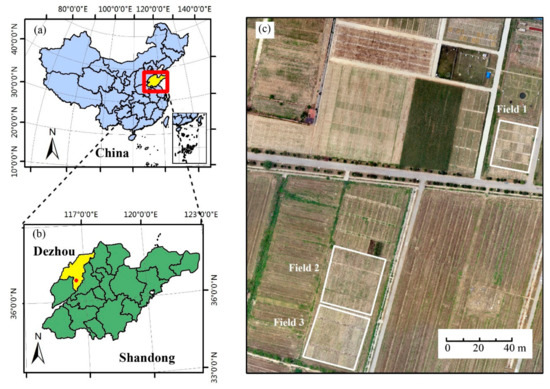
Figure 1.
(a) Location of Shandong Province in China; (b) location of the Yucheng Comprehensive Experiment Station (YCES, Chinese Academy of Sciences) in Shandong Province; (c) Overview of the three long-term experimental fields in YCES.
Three types of long-term experimental fields (89 plots in total, n1 = 25, n2 = 32, n3 = 32) with different irrigation, fertilization, and tillage treatments were selected for UAV observation during the maize growing season of 2018. Detailed experimental treatments of each field are described in Table 1. The experimental fields were run over ten years, providing a perfect study area for UAV remote sensing observation due to the existing differences in crop traits that occur simultaneously due to enforced gradients in the soil, fertilizer, and irrigation treatments.

Table 1.
Treatments used in the three experimental fields.
2.2. Ground Measurements and UAV Flight Missions
2.2.1. Ground Measurements of AGB and CH
Ground measurements were conducted either on the same day or within one day of the UAV observations. In order to ensure the reasonability and typicality of study, maize with relatively uniform canopies outside the border areas of each plot was selected for the experiment. Maize plants were destructively collected on a random basis for AGB and CH measurements in the laboratory (Figure 2). Considering the plot size, five typical maize plants (outside the border areas) of each plot were cut for measurement. In total, 445 biomass plants were taken (89 plots × 5 samples/plot: Field 1 = 25 × 5, Field 2 = 32 × 5, Field 2 = 32 × 5).
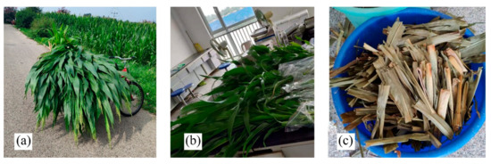
Figure 2.
(a) Destructive ground sampling in the field; (b) measurements of the above-ground biomass (AGB) of fresh maize in the laboratory; (c) the AGB of dry maize after removing the moisture.
CH (cm) was measured from the ground to the highest part of the plant using a straight tape. The average CH of the samples was calculated for each plot. After sampling, the whole plants, without roots, were immediately used for weighing the fresh AGB, after which the whole plant was then cut and dried at 105 °C for 2 h and then at 75 °C until the weight of the sample remained constant, in order to remove moisture for determining the dry matter. A total of 89 ground measured samples of maize fresh AGB, dry AGB, and CH were obtained. This weight was multiplied by the number of plants in each plot to obtain the AGB for each plot as follows:
where m (kg) is the total fresh/dry weight per maize plant; n is the number of crops per plot; and a (m) and b (m) are the width and length of each plot, respectively. The values for AGB were then rescaled to t·ha−1.
AGB (kg·m−2) = (m × n)/(a × b),
The fresh AGB (t·ha−1), dry AGB (t·ha−1), and CH (cm) datasets generated are given in Table 2. A high amount of variability can be seen in the datasets (i.e., cv (coefficient of variation), with a high sd (standard deviation)), because of the differences in tillage, irrigation, and treatment with nutrients or fertilizer. These statistical characteristics would be likely to contribute to a good fit between the measured and estimated values for AGB and CH.
Table 2.
Statistical summary of the in-situ measured crop above-ground biomass (AGB) (t·ha−1) and crop height (CH) (cm) (n = 89).
2.2.2. Acquisition and Pre-Processing of UAV Remote Sensing Data
Three UAV flight observation missions were executed on 22–24 July 2018, which is the time at the jointing period of the summer maize. The UAV flight was carried out between 09:30 and 14:30. The three types of UAV platforms (see Figure 3 for the EWZ-D6 six-rotator UAV (EWATT, Wuhan, China), the DJ M100 four-rotator UAV (SZ DJI Technology Co., Shenzhen, China), and the eBee wing-fixed UAV (SenseFly, Cheseaux-Lausanne, Switzerland) were equipped with three sensors—the Alpha Series AL3-32 LiDAR system (Phoenix, Los Angeles, CA, USA), the Micasense RedEdge-M (MicaSense, Seattle, WA, USA) multispectral camera, and the multiSPEC-4C multispectral camera (SenseFly, Cheseaux-Lausanne, Switzerland). Overlaps of imagery to the front and side were 65% and 85% for the multiSPEC-4C; 75% and 85% for the Micasense RedEdge-M; 70% and 70% for Alpha Series AL3-32. The flight heights were 120 m, 60 m, and 40 m for multiSPEC-4C, Micasense RedEdge-M, and Alpha Series AL3-32, respectively. Flights of the eBee, DJ M100, and EWATT UAVs were controlled by eMotion 3 (SenseFly, Cheseaux-Lausanne, Switzerland), Pix4D Capture (Pix4D, S.A., Lausanne, Switzerland), and Phoenix Flight Planner (Phoenix, Los Angeles, CA, USA), respectively. The field of view for LiDAR sensor was set to 270° and the scan rate was 700 k points/s.
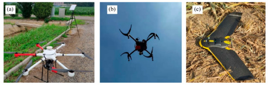
Figure 3.
Three unmanned aerial vehicles (UAV) platforms used in this study: (a) the EWZ-D6 Pro six-rotor UAV, (b) the DJI M100, and (c) the eBee wing-fixed UAV.
The Micasense RedEdge-M camera has five spectral channels (blue (B), green (G), red (R), red-edge (E), and near-infrared (NIR) bands) centered at 475 nm, 560 nm, 668 nm, 717 nm, and 840 nm, and with bandwidths of 20 nm, 20 nm, 10 nm, 10 nm, and 40 nm, respectively. The multiSPEC-4C camera has four specific spectral channels—G, R, E, and NIR bands situated at 550 nm, 660 nm, 735 nm, and 790 nm, with bandwidths of 40 nm, 40 nm, 10 nm, and 40 nm, respectively. The spatial resolutions of the images captured with the Micasense RedEdge-M and multiSPEC-4C cameras were 4 cm and 10 cm, respectively, which resulted in different spatial resolutions for the corresponding CH raster generated from the two multispectral SfM point clouds.
The CloudCompare open-source software was used to build CH raster data from the LiDAR point clouds (Figure 4a). For radiation correction of the multispectral data, the reflectance from a spectral panel was collected with each of the optical sensors before each flight. The radiation correction, image mosaic, and orthography of the UAV multispectral images were conducted using the Pix4D Mapper 3.1.22 (Pix4D, S.A., Lausanne, Switzerland). The DSM of the multispectral data was generated from SfM point clouds (Figure 4b) using Pix4D Mapper 3.1.22.
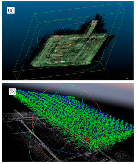
Figure 4.
(a) The Light Detection and Ranging (LiDAR) point clouds and (b) the multispectral Structure from Motion (SfM) point clouds of the study area.
The RGB images and CH raster datasets from the 89 experimental plots are shown in Figure 5 at three spatial resolutions (derived from the point clouds of the Alpha Series AL3-32, the Micasense RedEdge-M SfM, and the multiSPEC-4C SfM). ArcGIS 10.2 software (ESRI, Redlands, CA, USA), Python 2.7, and R × 64 3.5.3 were used for further data analysis and programming. To ensure a clear definition of the boundary of each plot for accurate data extraction under the coarse or medium spatial resolutions of the multispectral data (as shown in Figure 5b,c), the spectral data were superimposed onto the corresponding DSM data.
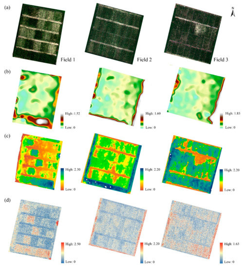
Figure 5.
(a) The RGB maps of three experimental fields; the crop height raster data based on (b) the multiSPEC-4C, (c) the Micasense RedEdge-M, and (d) the LiDAR point clouds.
2.3. Data Processing and Modeling
2.3.1. Generating Six Datasets
The data processing flowchart for the estimation of maize AGB by 3D UAV-based information at multi-spatial resolutions is shown in Figure 6. This process included three steps.
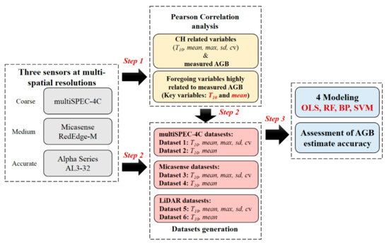
Figure 6.
Flowchart of this study to estimate the above-ground biomass (AGB) of maize using UAV-based multispectral SfM and LiDAR point clouds.
Firstly, to simplify the process used for estimating AGB in order to fulfill the requirements of agronomic application, we determined which key variables were highly correlated with AGB, using Pearson correlation coefficient analysis of the five statistical variables and the measurements of the fresh/dry AGB. These five variables included the mean value (mean), the mean value of the top 10% data (T10), standard deviation (sd), the coefficient of variation (cv), and the max value (max) of each plot, which were calculated from the CH datasets captured by the three sensors.
Secondly, six datasets were generated following the Pearson correlation coefficient analysis: Dataset 1 included five variables (mean, T10, sd, cv, and max) while Dataset 2 included the two key variables (mean and T10, please see Section 3.1 for the variable selections), both of which were derived from the multiSPEC-4C SfM point clouds. Dataset 3 also included five variables and Dataset 4 included the two key variables, both of which derived from the Micasense RedEdge-M SfM point clouds. Datasets 5 and 6 were analogous to the other datasets, but both were derived from the LiDAR point clouds.
Finally, the fresh and dry AGB of the maize were estimated using four methods—the statistical multiple linear regression model (OLS) and three widely used machine-learning methods (i.e., random forest (RF), backpropagation neural network (BP), and support vector machine (SVM))—using the six datasets generated during step 2.
2.3.2. Statistical Analysis and Methods Used for AGB Estimation
Four methods were used in this study to estimate the AGB of the maize—OLS, RF, BP, and SVM. The RF, BP, and SVM methods were run with the randomForest, the nnet, and the e1071 packages in R × 64 3.5.3, respectively. Each method included three steps. Firstly, all variables and the AGB were normalized to a mean of 0 and a standard deviation of 1.0 using the Scale function in R × 64 3.5.3. Secondly, the dataset was divided randomly into two sets, with the training dataset used for training and the other used as the testing dataset. Each method was run by applying leave-one-out-cross validation (LOOCV). LOOCV used N-1 samples as the training dataset and 1 sample as the testing dataset, then repeated modeling N times; thus 89 models were developed for each method in this study. Finally, the testing dataset was used for assessing the performance of each method in estimating the maize AGB.
Linear regression analysis was carried out between the estimated and measured values for AGB, and the models were then evaluated using the determining coefficient (R2), the root mean square error (RMSE), and the mean relative error (MRE):
where i represents the serial number of the sample, and Mi and Ei represent the measured and estimated AGB of the ith sample, respectively.
3. Results
3.1. Generating Multi-Source UAV-Based Datasets at Multi-Spatial Resolutions
Firstly, to simplify the process for estimating AGB, the Pearson correlation coefficient analysis was used to determine the key variables. Figure 7 shows the Pearson correlation coefficient analysis between the 3D information and the measured AGB/CH (n = 89). The results show that CH correlated significantly with both the fresh and dry AGB, with r values of 0.92 and 0.90 (p < 0.01, n = 89), respectively, indicating that using CH as an important 3D parameter of canopy structure was feasible for AGB estimation. Among the five 3D variables, the mean and T10 showed the highest correlations with CH with r values over 0.69, 0.81, and 0.83 (p < 0.01, n = 89) for the multiSPEC-4C, the Micasense RedEdge-M, and the LiDAR data, respectively. Max showed only a moderate relationship to CH, with r values of 0.51, 0.81, and 0.41 (p < 0.01, n = 89), respectively. The other parameters (i.e., cv and σ) were all only minimally related to CH.
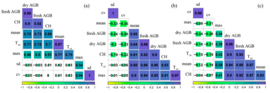
Figure 7.
Pearson correlation coefficient (r value) between the 3D statistical variables from (a) the multiSPEC-4C, (b) the Micasense RedEdge-M, and (c) the LiDAR point clouds and the ground-measured fresh AGB/dry AGB/Crop height (CH).
Furthermore, among the five variables calculated from the 3D point clouds, T10 and mean were also correlated significantly with fresh AGB, with r values of 0.72 and 0.73 (p < 0.01, n = 89) for the multiSPEC-4C data, 0.86 and 0.85 (p < 0.01, n = 89) for the Micasense RedEdge-M data, and 0.82 and 0.88 (p < 0.01, n = 89) for the LiDAR data. T10 and mean also showed a good relationship with dry AGB, which was analogous to fresh AGB.
3.2. AGB Estimate Using 3D Point Clouds at Multi-Spatial Resolutions
3.2.1. AGB Estimate Based on the multiSPEC-4C Data
The accuracy in estimating AGB using the multi-variable linear statistical model and machine learning methods was evaluated with R2, RMSE, and MRE (Table 3 and Figure 8). Except for BP, the accuracy in estimation using these methods with Dataset 1 (max, sd, cv, mean, and T10) (0.41 ≤ R2 ≤ 0.51, 5.02 ≤ RMSE ≤ 5.49, 0.53 ≤ MRE ≤ 0.55) was close to that of Dataset 2 (mean and T10) (0.44 ≤ R2 ≤ 0.49, 5.06 ≤ RMSE ≤ 5.36, 0.47 ≤ MRE ≤ 0.52). The R2 values for dry AGB were 0.45–0.53 and 0.39–0.48 using Dataset 1 and Dataset 2, respectively. The RMSE values for dry AGB were 0.57–0.62 and 0.63–0.69 using Dataset 1 and Dataset 2, respectively. These results suggest that the accuracy in the estimation of maize AGB using all four methods with 3D information from the multiSPEC-4C point clouds was low, and the accuracy of these two datasets was close.
Table 3.
R2, root mean square error (RMSE), and mean relative error (MRE) for linear regression between measured fresh/dry AGB and estimated fresh/dry AGB based on the multiSPEC-4C SfM point clouds using four algorithms (n = 89).
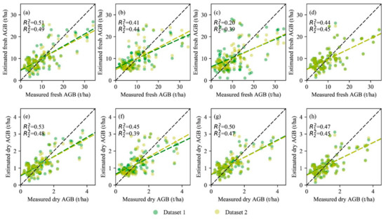
Figure 8.
Comparisons of measured AGB and estimated AGB of maize via the four methods based on Dataset 1 (green spots) and Dataset 2 (yellow spots), which were derived from the multiSPEC-4C SfM point clouds: (a–d) the traditional multi-variable linear regression model (OLS), random forest (RF), backpropagation neural network (BP), and support vector machine (SVM) methods for the AGB estimation of fresh maize; (e–h) OLS, RF, BP, and SVM for the AGB estimation of dry maize. R12 and R22 represent the coefficients of determination for a linear regression model between the measured and estimated AGB using Datasets 1 and 2, respectively.
Comparing the four methods in this study, it is apparent that except for when the BP method was used for estimating fresh AGB, there were no obvious differences in the results, as the R2, RMSE, and MRE values of the different methods were close. Additionally, there was no obvious advantage in using the machine learning methods over the traditional OLS method, as the R2, RMSE, and MRE values generated by use of the OLS method were 0.51, 5.02, and 0.53, which are slightly more accurate than those from the machine learning methods (e.g., for RF in fresh AGB estimate, R2 = 0.41, RMSE = 5.49, MRE = 0.53).
3.2.2. AGB Estimate Based on the Micasense RedEdge-M Data
The evaluations of the accuracy in estimating maize AGB with methods using Micasense RedEdge-M SfM point clouds are given in Table 4. Figure 9 shows the scatter of the measured and estimated AGB. The R2, RMSE, and MRE values of methods for estimating fresh AGB using Dataset 3 were 0.64–0.77, 3.41–4.48, and 0.30–0.43, respectively. Estimations made using Dataset 4 were slightly more accurate, with corresponding R2, RMSE, and MRE values of 0.67–0.77, 3.48–4.15, and 0.29–0.33, respectively. The accuracy in estimating dry AGB using all four methods with Dataset 4 increased slightly as compared to Dataset 3, with an increase in the R2 values of 0.02, 0.03, 0.02, and 0.02, decreases of 0.01, 0.02, 0.01, and 0.01 in the RMSE values, and MRE values that decreased by 0.01, 0.02, 0.01, and 0.01 for the OLS, RF, BP, and SVM methods, respectively.
Table 4.
R2, RMSE, and MRE for linear regression between measured fresh/dry AGB and estimated fresh/dry AGB based on the Micasense RedEdge-M SfM point clouds using four algorithms (n = 89).
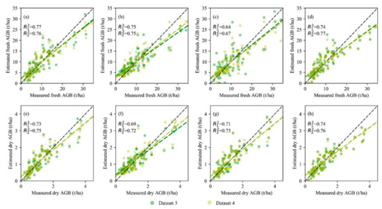
Figure 9.
Comparisons of measured AGB and estimated AGB of maize via the four methods based on Dataset 3 (green spots) and Dataset 4 (yellow spots), which were derived from the Micasense RedEdge-M SfM point clouds: (a–d) OLS, RF, BP, and SVM for the AGB estimation of fresh maize; (e–h) OLS, RF, BP, and SVM for the AGB estimation of dry maize. R12 and R22 represent the coefficient of determination for a linear regression model between the measured and estimated AGB using Datasets 3 and 4, respectively.
By comparing the estimation accuracy using the OLS method with the three machine learning methods, it was found that the BP methods performed less accurately than the others, while OLS and SVM performed slightly better and were more robust, with R2 values of approximately 0.75 for both fresh and dry AGB estimation.
3.2.3. AGB Estimate Based on the LiDAR Data
The evaluations of accuracy in the AGB estimation of the four methods using the LiDAR point clouds are given in Table 5, and the scatters of the measured AGB versus estimated AGB are shown in Figure 10. For fresh AGB, the R2, RMSE, and MRE values of the methods using Dataset 5 were 0.70–0.85, 2.72–4.01, and 0.25–0.34, respectively. Analogous to the AGB estimate using the Micasense RedEdge-M data, the accuracy of the fresh AGB estimate for Dataset 6 was more accurate, as the R2 values increased by 0.01, 0.07, 0.19, and 0, the RMSE values decreased by 0.02, 0.89, 1.65, and 0, and the MRE values also decreased by 0, 0.07, 0.12, and 0.02 for the OLS, RF, BP, and SVM methods, respectively, compared to those of Dataset 5. Dataset 6 also performed slightly better than Dataset 5 for dry AGB estimation.
Table 5.
R2, RMSE, and MRE for linear regression between measured fresh/dry AGB and estimated fresh/dry AGB based on the LiDAR point clouds using four algorithms (n = 89).
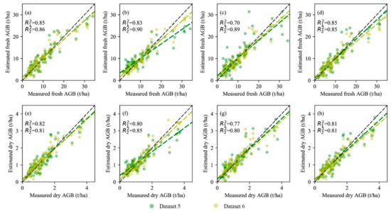
Figure 10.
Comparisons of measured AGB and estimated AGB of maize via the four methods based on Dataset 5 (green spots) and Dataset 6 (yellow spots), which were derived from the LiDAR point clouds: (a–d) OLS, RF, BP, and SVM for the AGB estimation of fresh maize; (e–h) OLS, RF, BP, and SVM for the AGB estimation of dry maize. R12 and R22 represent the coefficient of determination for a linear regression model between the measured and estimated AGB using Datasets 5 and 6, respectively.
Comparing the accuracy in the estimations made using the four methods in this study, the accuracy using the machine learning and OLS methods were close, except for the BP method when related to Dataset 5. Use of the RF method on Dataset 6 achieved the highest accuracy in this study, with R2, RMSE, and MRE values of 0.90, 2.29, 0.22 for estimation of the fresh AGB estimate, and 0.85, 0.33, and 0.23 for the dry AGB estimate.
3.3. Comparing the AGB Estimate Accuracy of the 3D Data with Multi-Spatial Resolutions
As can be seen in Figure 11, higher values of R2 and lower values of RMSE and MRE represent a higher accuracy in the estimation of AGB. Except for the results of the estimate for the AGB of dry maize using multiSPEC-4C data, the R2 values of the datasets (Datasets 2, 4, 6) which included two variables (T10 and mean) were slightly higher compared to those for the corresponding datasets (Datasets 1, 3, 5) when all the variables were included (mean, T10, sd, cv, and max). This was particularly relevant in the LiDAR datasets, where the R2 value using the RF method with Dataset 6 increased by 0.07. The RMSE and MRE values of Datasets 2, 4, and 6 decreased slightly compared to those of Datasets 1, 3, and 5, respectively, suggesting that those datasets that included only the two key variables sensitive to AGB performed slightly better than those including all the statistical variables.
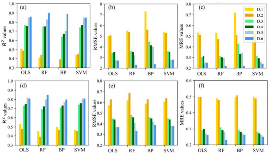
Figure 11.
Comparison of the accuracy of AGB estimation for the four methods using Dataset 1 (multiSPEC-4C—five variables), Dataset 2 (multiSPEC-4C—T10 and mean), Dataset 3 (Micasense RedEdge-M—five variables), Dataset 4 (Micasense RedEdge-M—T10 and mean), Dataset 5 (LiDAR—five variables), and Dataset 6 (LiDAR—T10 and mean): (a) R2, (b) RMSE, and (c) MRE of the maize fresh AGB estimate; (d) R2, (e) RMSE, and (f) MRE of the maize dry AGB estimate. (D.1 represents Dataset 1).
In this study, the values for R2, RMSE, and MRE for the OLS method were close to those of the RF and SVM machine learning methods, indicating that machine learning methods have no effective advantage over the traditional OLS method. Among the three machine learning methods, the performance of the BP method was poor when compared with the other methods, while RF and SVM performed better and were more robust.
Comparing datasets at multi-spatial scales, the R2 values of the multiSPEC-4C datasets at coarse spatial resolution (Datasets 1 and 2) were approximately 0.45, while those of Micasense RedEdge-M datasets at medium spatial resolution (Datasets 3 and 4) were 0.70–0.75, and those of the LiDAR datasets at high spatial resolution (Datasets 5 and 6) approached 0.85. The RMSE and MRE values decreased as the spatial resolution of the CH raster datasets increased. These results suggest that the spatial resolution of the CH raster datasets was a key variable that affected the results of the AGB estimation. The coarse spatial resolution of these datasets would have limited the capability for accurate crop monitoring and the estimation of parameters, while high spatial resolution contributed to more accurate estimates of the biophysical variables.
4. Discussion
Our research indicated that the 3D information from multispectral and LiDAR point clouds was an alternative means of estimating the fresh and dry AGB of crops. The spatial resolution of the crop height datasets was identified as a key factor affecting the accuracy of AGB estimates, as the high spatial resolution of the datasets contributed to accurate results in AGB estimation. Datasets generated by key variables that were highly correlated with AGB performed slightly better than those generated from all of the statistical variables. There was also no obvious difference between results from the three widely used machine learning methods (BP, RF, and SVM) and the traditional multi-variable linear regression model (OLS) in terms of the results for AGB estimation; however, the SVM and RF methods performed slightly more accurately and were more robust than BP in this study. The R2 values were approximately 0.45 for the AGB estimation from Datasets 1 and 2 (coarse, multiSPEC-4C datasets), 0.70–0.75 for Datasets 3 and 4 (medium, Micasense RedEdge-M), and those for Datasets 5 and 6 (high, LiDAR) approached 0.85.
4.1. Effects of the 3D Information on AGB Estimation
In recent years, the fusion of multi-source remote sensing data has been widely applied for the monitoring of vegetation, land cover, and the classification of species. Hyperspectral and 3D data (especially LiDAR data) are already in wide use for the estimation of forest biomass [26]. Generally, hyperspectral data are applied for classification, while LiDAR data are used for estimating the AGB of specific vegetation. Compared to the forest ecosystem, the vegetation species of farmland ecosystems are relatively singular because of the intervention of tillage. This means that the observation sensors onboard UAVs should be selected appropriately, in accordance with the practical requirements.
For further analyzing the effects of using 3D information on the AGB estimate, we conducted fresh/dry AGB estimates based on the Micasense RedEdge-M spectral datasets (A-Dataset 1) and the fusion datasets (fusion of the spectral data and Micasense RedEdge-M SfM point clouds, A-Dataset 2) using the OLS, RF, BP, and SVM methods. The scatters of the measured and estimated AGB are given in Figure 12. The performance of the estimation of the AGB from the two A-Datasets are compared in Figure 13.
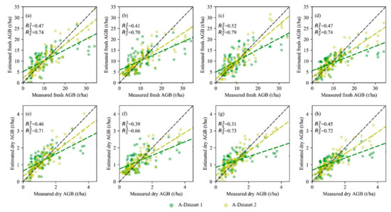
Figure 12.
Comparisons of measured AGB and estimated AGB of maize via four methods based on A-Dataset 1 (green spots) and A-Dataset 2 (yellow spots) that were derived from the spectral data and fusion data, respectively: (a–d) OLS, RF, BP, and SVM for the AGB estimation of fresh maize; (e–h) OLS, RF, BP, and SVM for the AGB estimation of dry maize. R12 and R22 represent the coefficient of determination for a linear regression model between the measured and estimated AGB using A-Dataset 1 and A-Dataset 2, respectively.
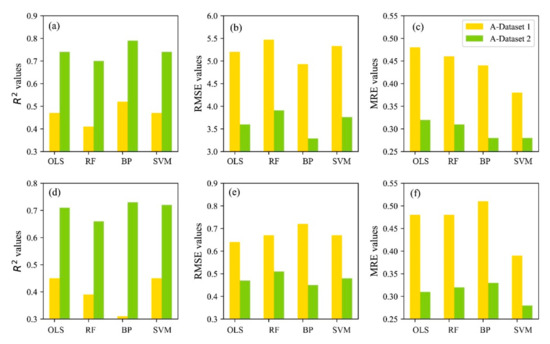
Figure 13.
Comparison of the accuracy of AGB estimation for the four methods using A-Dataset 1 (Spectral information), A-Dataset 2 (fusion of spectral data and the 3D multispectral SfM point clouds (T10 and mean)): (a) R2, (b) RMSE, and (c) MRE of fresh AGB; (d) R2, (e) RMSE, and (f) MRE of dry AGB.
The R2, RMSE, and MRE values of the four methods using A-Dataset 1 were approximately 0.45, 5.20, and 0.45 for the fresh AGB, and 0.40, 0.67, and 0.50 for the dry AGB, suggesting that the use of spectral information did not perform well for AGB estimation. Moreover, as Figure 12 shows, all four methods underestimated the AGB when the AGB values were above 20 t·ha−1 and 2.1 t·ha−1 for the fresh and dry AGB of the maize, respectively, indicating that there were saturation limitations in the spectral data when the canopy coverage was medium to high.
In this study, maize was cultivated in different plots using various tillage treatments, nutrient levels, and soil moisture content. Plants in the plots with nutrients and water deficiencies suffered from lower chlorophyll content in the leaves and a lower LAI, resulting in different growth periods, which may have contributed to the poor performances in estimation when using spectral information [39]. Viewing and illumination geometry could also affect the optical measurement of natural surfaces because of the anisotropic reflectance properties of vegetation [40]. Information concerning the canopy structure cannot be obtained with optical cameras. This is because as plant density increases, adjacent leaves overlap, resulting in structural information that is inaccessible to optical cameras [25]. Additionally, the maize AGB measured in this study included more photosynthetically inactive components (e.g., stems) than leaf biomass. These inactive components are likely to affect the relationship between spectral reflectance and maize AGB. Therefore, the spectral information was insufficient for accurate AGB estimation.
Kross et al. (2015) pointed out that cumulative VIs calculated via logistic function were better for estimating AGB, because of the capability of cumulative indices to reflect biochemical properties [12]. Therefore, implementing multi-phase UAV flights for obtaining cumulative VIs may be an alternative way to improve the AGB estimate using UAV-based spectral information. Short-wavelength infrared (SWIR) could be an alternative use for avoiding problems with saturation [41,42]. However, in this study, we emphasized the contribution of 3D information on the estimation of maize AGB.
Comparing the performances of A-Datasets 1 and 2, the R2 values for the methods using A-Dataset 2 (fusion datasets) were ≥ 0.63 for the fresh AGB estimate (≥ 0.62 for dry AGB), while those of A-Dataset 1 were approximately 0.45 and 0.40 for the fresh and dry AGB estimates, respectively. These results indicate that the use of 3D information about a vegetation canopy could effectively improve the accuracy of AGB estimation. Previous studies have demonstrated that crop CH could be used to accurately estimate crop AGB [3,43], since CH represents 3D information about a canopy and 3D information might overcome the saturation and physical/biological losses encountered when using spectral reflectance.
The narrow bands have already demonstrated an excellent relationship with crop biomass [41], as they can provide abundant spectral information, which complements information about the canopy structure derived from the UAV-based 3D information.
4.2. Performances of Two Type Datasets for AGB Estimate
Crop height has proven to be a critical indicator of AGB [44]. Many studies have investigated the effects of some of the statistical variables calculated from CH on crop parameter estimation [33,45]. In this study, the Pearson correlation analysis showed that, among all the statistical variables calculated from the multispectral SfM and LiDAR point clouds, T10 (the mean value of top 10% data) and mean were the two key variables found to have a significant positive correlation with maize fresh/dry AGB, while the max values were only moderately correlated with AGB. The other variables (cv and sd) were only marginally related to AGB.
The canopy volume within each plot could be obtained from multiplying the mean value of CH by the area of each plot. The plots used for this study were 50 m2 for Field 2 and 3, and 30 m2 for Field 1. Therefore, the mean value for CH can represent the canopy volume, which shows the average growth status of plants in the plot, as well as including more 3D information about the crops, such as the breast diameter (DBH) of the plants. The T10 represents the crop height, which has a significantly positive correlation with crop AGB (see Figure 7, the r values between the fresh/dry AGB and CH were 0.92 and 0.90, respectively, p < 0.01, n = 89). Therefore, T10 is another important variable that can be used for AGB estimation.
The max value is the value of the highest point of each plot, representing the height of the tallest maize within each plot, which does not represent the average level of CH in each plot. However, owing to the strict agronomic practices, the canopies were relatively uniform within each plot, so the max parameter showed only a medium correlation with fresh/dry AGB.
The cv and sd show the differences in crop growth within each plot. However, as the maize is grown in rows and the sampling was carried out during the jointing stage of maize, when most of the maize has not yet been ridged, the cv and sd might be affected by environmental noise, such as the soil background. Therefore, Datasets 2, 4, and 6, which included two key variables (mean and T10), showed a higher accuracy for the estimation of maize AGB than Datasets 1, 3, and 5, which included all five statistical variables. Previous studies have also demonstrated that the mean value is of higher importance for AGB estimation by regression models than other statistical variables [45]. However, the effects of more input variables into regression models remain unclear. This is because more input variables in regression models could provide more information about the vegetation, which should be helpful for AGB estimation. Therefore, this issue needs to be further validated in future studies.
4.3. Effects of Spatial Resolution of Datasets on AGB Estimate
The spatial resolution of the datasets, which was related to the density of the point clouds, has been proven to affect biomass estimation [32]. In this study, the LiDAR datasets performed best for AGB estimation, with the most accurate results, while the performance of the multiSPEC-4C SfM point clouds was limited due to their coarse spatial resolution. The Micasense RedEdge-M SfM point clouds performed moderately in AGB estimation. These results may be caused by some of the following reasons.
Firstly, CH was measured from the ground to the highest point of the leaf or the male ear of maize in the state of natural growth, and the spatial structure at the highest point was small, which could lead to such measurements being mistaken as noise and removed by the DSM construction algorithm. Secondly, the passive multispectral sensors (RGB and multispectral cameras) had no capacity to penetrate dense canopy, leading to errors in generating digital terrain models [27]. Thirdly, an adequate number of ground control points (GCPs) and a high overlap of the individual images are necessary to ensure image accuracy during the photogrammetric process [46]. The bias introduced by the use of different levels of sampling might be another reason. In this study, the destructive sampling of the maize AGB and CH were measured at the level of a single plant and at distinct locations within the plot. However, the spatial resolution of the multispectral cameras, especially the multiSPEC-4C sensor, was too coarse to generate accurate DSM at the plant level when flown on a UAV. The average CH value of the whole plot was used for analysis. Therefore, compared to the LiDAR point clouds, the two multispectral SfM point clouds showed a lower capacity for AGB estimation.
When working with LiDAR or other multispectral sensors onboard UAVs, we face the challenge of cost versus estimation accuracy for parameters concerning vegetation. Considering the high costs of LiDAR systems, many researchers prefer to use multispectral sensors to generate SfM point clouds, or RGB-Depth cameras (e.g., Microsoft Kinect V2) [7] for the extraction of 3D information about a vegetation canopy [26,29]. Precise CH extraction can be achieved when the spatial resolution of the optical images is high [47]. Reducing the altitude of the UAV or choosing cameras with definite spatial resolutions are effective ways that such specific requirements can be fulfilled. The former can be compensated by adapting the flight plan to the desired ground spatial resolution, but the flight coverage will decrease as a result of the limited flight time of current UAV batteries. Therefore, future studies should investigate what resolutions are actually required for specific applications in order to further perfect the agronomic schemes.
In this study, the mean value was used to present the volume of vegetation within each plot. However, more precise methods for the estimation of a canopy volume need to be developed in the future, such as building alpha shapes which represent the outline surrounding a set of 3D points [7], to further improve the accuracy and robustness of crop monitoring and vegetation parameter estimation.
4.4. Performances of Four Methods on AGB Estimate
The results of this study showed that the three commonly used machine learning methods (RF, BP, and SVM) had no advantage over the OLS method. As Figure 14 showed, the CH and measured AGB have a linear relationship, with R2 values of 0.83 and 0.81 for fresh and dry AGB, respectively, so the multi-variable linear regression method (OLS) could be used to accurately estimate maize AGB.
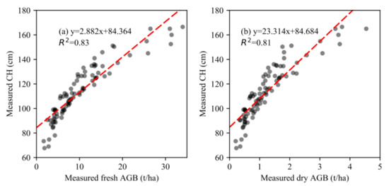
Figure 14.
Scatter plots of measured crop height and measured maize (a) fresh AGB and (b) dry AGB (n = 89).
The three machine learning methods used in this study have specific advantages and characteristics. For example, RF is insensitive to noise or over-fitting [12], and is able to solve problems concerning multi-collinearity [48]; BP can modify algorithms quickly but requires a large number of samples; SVM takes advantage of dealing with limited samples and high dimensional datasets. Comparing the results of AGB estimation using these three methods, the SVM and RF methods were found to be more robust for AGB estimation, which is consistent with the results of previous studies [35]. This is because BP is often applied to large amounts of sampling data, while SVR and RF methods are more suitable for smaller samples.
Furthermore, the traditional statistical regression models and machine-learning models used in this study have been widely employed for the retrieval/estimates of the biophysical and biochemical parameters of crops (e.g., leaf area index [22,49], chlorophyll content [5], and crop yield [8]). However, one of the main limitations is that the application of these methods is valid only in the areas for which they have been calibrated [50,51]. Previous studies have demonstrated that models based on pseudo-waveform variables estimate AGB more accurately [45,52]. However, it essential to consider accuracy along with the complexity of the methods used for estimation in practical application. The results of this study have demonstrated that using 3D statistical variables could meet the requirements for accuracy in the AGB estimation of precision agriculture. Therefore, we recommend this simple, robust, and accurate method for agronomic applications.
Regarding the estimation of vegetation AGB based on 3D information of UAV remote-sensing, previous studies have already successfully applied UAV-based 3D information to forest ecosystems. However, in recent years, this 3D information has gradually been applied to crops (e.g., wheat [48,53], rice [54], maize [43]) and grassland [55] for plant height extraction and AGB estimation. This study further demonstrated that the use of 3D point clouds from multispectral and LiDAR systems were effective and robust for estimating crop AGB. The high spatial resolution of 3D datasets was essential to improve the accuracy of AGB estimation. Moreover, three commonly applied machine learning methods (RF, BP, SVM) did not show any obvious advantage over the traditional multiple linear regression model (OLS), while the RF and SVM methods are recommended for AGB estimation owing to their robustness and accuracy.
5. Conclusions
This study used UAV-based 3D information (the multispectral SfM (from Micasense RedEdge-M and multiSPEC-4C cameras) and LiDAR point clouds (Alpha Series AL3-32 sensor)) at multi-spatial resolutions to estimate the fresh and dry above-ground biomass of maize through the traditional multi-variable linear regression model (OLS) and three machine learning methods (RF, BP, and SVM). The results of this study demonstrated that crop height was an essential parameter for the accurate estimation of AGB, and that the high spatial resolution of CH datasets is therefore a key factor for precise maize AGB estimation. Among the five statistical variables used in this study, the mean and T10 of CH datasets showed the highest correlation with crop biomass, and the datasets including only these two variables performed slightly better than those including all statistical variables. Additionally, both the OLS method and the three machine learning methods performed well in AGB estimation, but the SVM and RF methods were slightly better, and these are therefore recommended for maize AGB estimation.
The results of this study suggest that crop height is an alternative and more robust way for estimating the AGB of maize, and multispectral SfM point clouds with high spatial resolution could fulfill the requirements for estimates concerning other crop parameters, which is preferred for agronomic applications, owing to the low cost and satisfactory accuracy in estimation.
Author Contributions
Z.S., X.L. and Y.H. acquired the funding for UAV flight missions and ground measurements. Z.S., W.Z. and Y.H. developed the workflow for this study. W.Z., J.P., J.Z. and B.Y. conducted UAV flight missions and processed UAV data. J.L. developed a part of experimental plots with different treatments. W.Z. conducted field experiments. W.Z. and Z.S. analyzed the data and wrote the paper.
Funding
This study was supported by the Key Projects of the Chinese Academy of Sciences (KFZD-SW-319), the National Natural Science Foundation of China (31570472, 31870421, 41771388), the Science and Technology Service Network Initiative of the Chinese Academy of Sciences (KFJ-STS-ZDTP-049), the Strategic Priority Research Program of the Chinese Academy of Sciences (XDA19040303), and the National Key Research and Development Program of China (2017YFC0503805).
Acknowledgments
Thanks for assistance provided by Qi Liu, Zhenmin Liu, Guicang Ma, and Xuezhi Yue for assistant of UAV flight missions, and Yinxia Zhu, Yansheng Han for assistant of field measurements.
Conflicts of Interest
The authors declare no conflict of interest.
References
- Lobell, D.B.; Field, C.B. Global scale climate–crop yield relationships and the impacts of recent warming. Environ. Res. Lett. 2007, 2, 014002. [Google Scholar] [CrossRef]
- Licker, R.; Johnston, M.; Foley, J.A.; Barford, C.; Kucharik, C.J.; Monfreda, C.; Ramankutty, N. Mind the gap: How do climate and agricultural management explain the ‘yield gap’ of croplands around the world: Investigating drivers of global crop yield patterns. Glob. Ecol. Biogeogr. 2010, 19, 769–782. [Google Scholar] [CrossRef]
- Yue, J.; Yang, G.; Li, C.; Li, Z.; Wang, Y.; Feng, H.; Xu, B. Estimation of Winter Wheat Above-Ground Biomass Using Unmanned Aerial Vehicle-Based Snapshot Hyperspectral Sensor and Crop Height Improved Models. Remote Sens. 2017, 9, 708. [Google Scholar] [CrossRef]
- Yang, G.; Liu, J.; Zhao, C.; Li, Z.; Huang, Y.; Yu, H.; Xu, B.; Yang, X.; Zhu, D.; Zhang, X.; et al. Unmanned Aerial Vehicle Remote Sensing for Field-Based Crop Phenotyping: Current Status and Perspectives. Front. Plant Sci. 2017, 8, 8. [Google Scholar] [CrossRef]
- Roosjen, P.P.J.; Brede, B.; Suomalainen, J.M.; Bartholomeus, H.M.; Kooistra, L.; Clevers, J.G.P.W. Improved estimation of leaf area index and leaf chlorophyll content of a potato crop using multi-angle spectral data – potential of unmanned aerial vehicle imagery. Int. J. Appl. Earth Obs. Geoinf. 2018, 66, 14–26. [Google Scholar] [CrossRef]
- Lu, B.; He, Y.; Liu, H.H.T. Mapping vegetation biophysical and biochemical properties using unmanned aerial vehicles-acquired imagery. Int. J. Remote Sens. 2018, 39, 5265–5287. [Google Scholar] [CrossRef]
- Rueda-Ayala, V.P.; Pena, J.M.; Hoglind, M.; Bengochea-Guevara, J.M.; Andujar, D. Comparing UAV-Based Technologies and RGB-D Reconstruction Methods for Plant Height and Biomass Monitoring on Grass Ley. Sensors 2019, 19, 535. [Google Scholar] [CrossRef] [PubMed]
- Battude, M.; Al Bitar, A.; Morin, D.; Cros, J.; Huc, M.; Marais Sicre, C.; Le Dantec, V.; Demarez, V. Estimating maize biomass and yield over large areas using high spatial and temporal resolution Sentinel-2 like remote sensing data. Remote Sens. Environ. 2016, 184, 668–681. [Google Scholar] [CrossRef]
- Casas, A.; Riaño, D.; Ustin, S.L.; Dennison, P.; Salas, J. Estimation of water-related biochemical and biophysical vegetation properties using multitemporal airborne hyperspectral data and its comparison to MODIS spectral response. Remote Sens. Environ. 2014, 148, 28–41. [Google Scholar] [CrossRef]
- Castaldi, F.; Casa, R.; Pelosi, F.; Yang, H. Influence of acquisition time and resolution on wheat yield estimation at the field scale from canopy biophysical variables retrieved from SPOT satellite data. Int. J. Remote Sens. 2015, 36, 2438–2459. [Google Scholar] [CrossRef]
- Soudani, K.; François, C.; le Maire, G.; Le Dantec, V.; Dufrêne, E. Comparative analysis of IKONOS, SPOT, and ETM+ data for leaf area index estimation in temperate coniferous and deciduous forest stands. Remote Sens. Environ. 2006, 102, 161–175. [Google Scholar] [CrossRef]
- Kross, A.; McNairn, H.; Lapen, D.; Sunohara, M.; Champagne, C. Assessment of RapidEye vegetation indices for estimation of leaf area index and biomass in corn and soybean crops. Int. J. Appl. Earth Obs. Geoinf. 2015, 34, 235–248. [Google Scholar] [CrossRef]
- Hunt, E.R.; Horneck, D.A.; Spinelli, C.B.; Turner, R.W.; Bruce, A.E.; Gadler, D.J.; Brungardt, J.J.; Hamm, P.B. Monitoring nitrogen status of potatoes using small unmanned aerial vehicles. Precis. Agric. 2018, 19, 314–333. [Google Scholar] [CrossRef]
- Li, Z.; Huang, C.; Zhu, Z.; Gao, F.; Tang, H.; Xin, X.; Ding, L.; Shen, B.; Liu, J.; Chen, B.; et al. Mapping daily leaf area index at 30 m resolution over a meadow steppe area by fusing Landsat, Sentinel-2A and MODIS data. Int. J. Remote Sens. 2018, 39, 9025–9053. [Google Scholar] [CrossRef]
- Sankey, T.; Donager, J.; McVay, J.; Sankey, J.B. UAV lidar and hyperspectral fusion for forest monitoring in the southwestern USA. Remote Sens. Environ. 2017, 195, 30–43. [Google Scholar] [CrossRef]
- Zhang, C.; Kovacs, J.M. The application of small unmanned aerial systems for precision agriculture: A review. Precis. Agric. 2012, 13, 693–712. [Google Scholar] [CrossRef]
- Jiao, Q.; Zhang, B.; Liu, J.; Liu, L. A novel two-step method for winter wheat-leaf chlorophyll content estimation using a hyperspectral vegetation index. Int. J. Remote Sens. 2014, 35, 7363–7375. [Google Scholar] [CrossRef]
- Berger, K.; Atzberger, C.; Danner, M.; D’Urso, G.; Mauser, W.; Vuolo, F.; Hank, T. Evaluation of the PROSAIL Model Capabilities for Future Hyperspectral Model Environments: A Review Study. Remote Sens. 2018, 10, 85. [Google Scholar] [CrossRef]
- Wei, S.; Fang, H. Estimation of canopy clumping index from MISR and MODIS sensors using the normalized difference hotspot and darkspot (NDHD) method: The influence of BRDF models and solar zenith angle. Remote Sens. Environ. 2016, 187, 476–491. [Google Scholar] [CrossRef]
- Muñoz, J.D.; Finley, A.O.; Gehl, R.; Kravchenko, S. Nonlinear hierarchical models for predicting cover crop biomass using Normalized Difference Vegetation Index. Remote Sens. Environ. 2010, 114, 2833–2840. [Google Scholar] [CrossRef]
- Zeng, Y.; Xu, B.; Yin, G.; Wu, S.; Hu, G.; Yan, K.; Yang, B.; Song, W.; Li, J. Spectral Invariant Provides a Practical Modeling Approach for Future Biophysical Variable Estimations. Remote Sens. 2018, 10, 1508. [Google Scholar] [CrossRef]
- Yao, X.; Wang, N.; Liu, Y.; Cheng, T.; Tian, Y.; Chen, Q.; Zhu, Y. Estimation of Wheat LAI at Middle to High Levels Using Unmanned Aerial Vehicle Narrowband Multispectral Imagery. Remote Sens. 2017, 9, 1304. [Google Scholar] [CrossRef]
- Serrano, L.; Filella, I.; Peñuelas, J. Remote Sensing of Biomass and Yield of Winter Wheat under Different Nitrogen Supplies. Crop Sci. 2000, 40, 723. [Google Scholar] [CrossRef]
- Bendig, J.; Yu, K.; Aasen, H.; Bolten, A.; Bennertz, S.; Broscheit, J.; Gnyp, M.L.; Bareth, G. Combining UAV-based plant height from crop surface models, visible, and near infrared vegetation indices for biomass monitoring in barley. Int. J. Appl. Earth Obs. Geoinf. 2015, 39, 79–87. [Google Scholar] [CrossRef]
- Ma, J.; Li, Y.; Chen, Y.; Du, K.; Zheng, F.; Zhang, L.; Sun, Z. Estimating above ground biomass of winter wheat at early growth stages using digital images and deep convolutional neural network. Eur. J. Agron. 2019, 103, 117–129. [Google Scholar] [CrossRef]
- González-Jaramillo, V.; Fries, A.; Bendix, J. AGB Estimation in a Tropical Mountain Forest (TMF) by Means of RGB and Multispectral Images Using an Unmanned Aerial Vehicle (UAV). Remote Sens. 2019, 11, 1413. [Google Scholar] [CrossRef]
- Aasen, H.; Burkart, A.; Bolten, A.; Bareth, G. Generating 3D hyperspectral information with lightweight UAV snapshot cameras for vegetation monitoring: From camera calibration to quality assurance. ISPRS J. Photogramm. Remote Sens. 2015, 108, 245–259. [Google Scholar] [CrossRef]
- Niu, Y.; Zhang, L.; Zhang, H.; Han, W.; Peng, X. Estimating Above-Ground Biomass of Maize Using Features Derived from UAV-Based RGB Imagery. Remote Sens. 2019, 11, 1261. [Google Scholar] [CrossRef]
- Bendig, J.; Bolten, A.; Bennertz, S.; Broscheit, J.; Eichfuss, S.; Bareth, G. Estimating Biomass of Barley Using Crop Surface Models (CSMs) Derived from UAV-Based RGB Imaging. Remote Sens. 2014, 6, 10395–10412. [Google Scholar] [CrossRef]
- Caruso, G.; Tozzini, L.; Rallo, G.; Primicerio, J.; Moriondo, M.; Palai, G.; Gucci, R. Estimating biophysical and geometrical parameters of grapevine canopies (‘Sangiovese’) by an unmanned aerial vehicle (UAV) and VIS-NIR cameras. VITIS J. Grapevine Res. 2017, 56, 63–70. [Google Scholar]
- Karpina, M.; Jarząbek-Rychard, M.; Tymków, P.; Borkowski, A. UAV-based automatic tree growth measurement for biomass estimation. ISPRS Int. Arch. Photogramm. Remote Sens. Spat. Inf. Sci. 2016, XLI-B8, 685–688. [Google Scholar] [CrossRef]
- Luo, S.; Wang, C.; Xi, X.; Pan, F.; Peng, D.; Zou, J.; Nie, S.; Qin, H. Fusion of airborne LiDAR data and hyperspectral imagery for aboveground and belowground forest biomass estimation. Ecol. Indic. 2017, 73, 378–387. [Google Scholar] [CrossRef]
- Cao, L.; Liu, H.; Fu, X.; Zhang, Z.; Shen, X.; Ruan, H. Comparison of UAV LiDAR and Digital Aerial Photogrammetry Point Clouds for Estimating Forest Structural Attributes in Subtropical Planted Forests. Forests 2019, 10, 145. [Google Scholar] [CrossRef]
- Brede, B.; Lau, A.; Bartholomeus, H.; Kooistra, L. Comparing RIEGL RiCOPTER UAV LiDAR Derived Canopy Height and DBH with Terrestrial LiDAR. Sensors 2017, 17, 2371. [Google Scholar] [CrossRef]
- Wang, L.; Zhou, X.; Zhu, X.; Dong, Z.; Guo, W. Estimation of biomass in wheat using random forest regression algorithm and remote sensing data. Crop J. 2016, 4, 212–219. [Google Scholar] [CrossRef]
- Dong, J.; Zhuang, D.; Huang, Y.; Fu, J. Advances in Multi-Sensor Data Fusion: Algorithms and Applications. Sensors 2009, 9, 7771–7784. [Google Scholar] [CrossRef]
- Cai, Y.; Guan, K.; Lobell, D.; Potgieter, A.B.; Wang, S.; Peng, J.; Xu, T.; Asseng, S.; Zhang, Y.; You, L.; et al. Integrating satellite and climate data to predict wheat yield in Australia using machine learning approaches. Agric. For. Meteorol. 2019, 274, 144–159. [Google Scholar] [CrossRef]
- Guo, L.; Sun, Z.; Ouyang, Z.; Han, D.; Li, F. A comparison of soil quality evaluation methods for Fluvisol along the lower Yellow River. Catena 2017, 152, 135–143. [Google Scholar] [CrossRef]
- Kanning, M.; Kühling, I.; Trautz, D.; Jarmer, T. High-Resolution UAV-Based Hyperspectral Imagery for LAI and Chlorophyll Estimations from Wheat for Yield Prediction. Remote Sens. 2018, 10, 2000. [Google Scholar] [CrossRef]
- Roosjen, P.; Suomalainen, J.; Bartholomeus, H.; Kooistra, L.; Clevers, J. Mapping Reflectance Anisotropy of a Potato Canopy Using Aerial Images Acquired with an Unmanned Aerial Vehicle. Remote Sens. 2017, 9, 417. [Google Scholar] [CrossRef]
- Gnyp, M.L.; Bareth, G.; Li, F.; Lenz-Wiedemann, V.I.S.; Koppe, W.; Miao, Y.; Hennig, S.D.; Jia, L.; Laudien, R.; Chen, X.; et al. Development and implementation of a multiscale biomass model using hyperspectral vegetation indices for winter wheat in the North China Plain. Int. J. Appl. Earth Obs. Geoinf. 2014, 33, 232–242. [Google Scholar] [CrossRef]
- Berni, J.A.J.; Zarco-Tejada, P.J.; Suarez, L.; Fereres, E. Thermal and Narrowband Multispectral Remote Sensing for Vegetation Monitoring from an Unmanned Aerial Vehicle. IEEE Trans. Geosci. Remote Sens. 2009, 47, 722–738. [Google Scholar] [CrossRef]
- Li, W.; Niu, Z.; Chen, H.; Li, D.; Wu, M.; Zhao, W. Remote estimation of canopy height and aboveground biomass of maize using high-resolution stereo images from a low-cost unmanned aerial vehicle system. Ecol. Indic. 2016, 67, 637–648. [Google Scholar] [CrossRef]
- Chang, A.; Jung, J.; Maeda, M.M.; Landivar, J. Crop height monitoring with digital imagery from Unmanned Aerial System (UAS). Comput. Electron. Agric. 2017, 141, 232–237. [Google Scholar] [CrossRef]
- Luo, S.; Wang, C.; Xi, X.; Nie, S.; Fan, X.; Chen, H.; Yang, X.; Peng, D.; Lin, Y.; Zhou, G. Combining hyperspectral imagery and LiDAR pseudo-waveform for predicting crop LAI, canopy height and above-ground biomass. Ecol. Indic. 2019, 102, 801–812. [Google Scholar] [CrossRef]
- Boccardo, P.; Chiabrando, F.; Dutto, F.; Tonolo, F.; Lingua, A. UAV Deployment Exercise for Mapping Purposes: Evaluation of Emergency Response Applications. Sensors 2015, 15, 15717–15737. [Google Scholar] [CrossRef]
- Jayathunga, S.; Owari, T.; Tsuyuki, S. Digital Aerial Photogrammetry for Uneven-Aged Forest Management: Assessing the Potential to Reconstruct Canopy Structure and Estimate Living Biomass. Remote Sens. 2019, 11, 338. [Google Scholar] [CrossRef]
- Yue, J.; Feng, H.; Jin, X.; Yuan, H.; Li, Z.; Zhou, C.; Yang, G.; Tian, Q. A Comparison of Crop Parameters Estimation Using Images from UAV-Mounted Snapshot Hyperspectral Sensor and High-Definition Digital Camera. Remote Sens. 2018, 10, 1138. [Google Scholar] [CrossRef]
- Dong, T.; Liu, J.; Shang, J.; Qian, B.; Ma, B.; Kovacs, J.M.; Walters, D.; Jiao, X.; Geng, X.; Shi, Y. Assessment of red-edge vegetation indices for crop leaf area index estimation. Remote Sens. Environ. 2019, 222, 133–143. [Google Scholar] [CrossRef]
- Becker-Reshef, I.; Vermote, E.; Lindeman, M.; Justice, C. A generalized regression-based model for forecasting winter wheat yields in Kansas and Ukraine using MODIS data. Remote Sens. Environ. 2010, 114, 1312–1323. [Google Scholar] [CrossRef]
- Houborg, R.; Boegh, E. Mapping leaf chlorophyll and leaf area index using inverse and forward canopy reflectance modeling and SPOT reflectance data. Remote Sens. Environ. 2008, 112, 186–202. [Google Scholar] [CrossRef]
- Muss, J.D.; Mladenoff, D.J.; Townsend, P.A. A pseudo-waveform technique to assess forest structure using discrete lidar data. Remote Sens. Environ. 2011, 115, 824–835. [Google Scholar] [CrossRef]
- Song, Y.; Wang, J. Winter Wheat Canopy Height Extraction from UAV-Based Point Cloud Data with a Moving Cuboid Filter. Remote Sens. 2019, 11, 1239. [Google Scholar] [CrossRef]
- Cen, H.; Wan, L.; Zhu, J.; Li, Y.; Li, X.; Zhu, Y.; Weng, H.; Wu, W.; Yin, W.; Xu, C.; et al. Dynamic monitoring of biomass of rice under different nitrogen treatments using a lightweight UAV with dual image-frame snapshot cameras. Plant Methods 2019, 15, 32. [Google Scholar] [CrossRef]
- Zhang, H.; Sun, Y.; Chang, L.; Qin, Y.; Chen, J.; Qin, Y.; Du, J.; Yi, S.; Wang, Y. Estimation of Grassland Canopy Height and Aboveground Biomass at the Quadrat Scale Using Unmanned Aerial Vehicle. Remote Sens. 2018, 10, 851. [Google Scholar] [CrossRef]
© 2019 by the authors. Licensee MDPI, Basel, Switzerland. This article is an open access article distributed under the terms and conditions of the Creative Commons Attribution (CC BY) license (http://creativecommons.org/licenses/by/4.0/).