Next-Generation Gravity Missions: Sino-European Numerical Simulation Comparison Exercise

Abstract

Temporal gravity retrieval simulation results of a future Bender-type double pair mission concept, performed by five processing centers of a Sino-European study team, have been inter-compared and assessed. They were computed in a synthetic closed-loop simulation world by five independent software systems applying different gravity retrieval methods, but were based on jointly defined mission scenarios. The inter-comparison showed that the results achieved a quite similar performance. Exemplarily, the root mean square (RMS) deviations of global equivalent water height fields from their true reference, resolved up to degree and order 30 of a 9-day solution, vary in the order of 10% of the target signal. Also, co-estimated independent daily gravity fields up to degree and order 15, which have been co-estimated by all processing centers, do not show large differences among each other. This positive result is an important pre-requisite and basis for future joint activities towards the realization of next-generation gravity missions.

1. Introduction

Next Generation Gravity Missions (NGGMs), expected to be launched in the midterm future, have set high anticipations for an enhanced monitoring of mass transport in the Earth system, establishing that their products are applicable to new scientific fields and serving societal needs. Past and current gravity missions such as Gravity Recovery and Climate Experiment (GRACE, [1]) and GRACE Follow-On [2] have improved our understanding of many mass change processes, such as the global water cycle, ice mass melting of ice sheets and glaciers, changes in ocean mass closely related to eustatic sea level rise, which are subtle indicators of climate change, but also gravity changes related to solid Earth processes such as big earthquakes or glacial isostatic adjustment (GIA). The Gravity field and steady-state Ocean Circulation Explorer (GOCE) mission [3] has improved our knowledge of long-term mass distribution and has provided the physical reference surface of the geoid, with a resolution down to 70–80 km.

The main objective of NGGMs is not only the continuation and extension of existing mass transport time series, but also a significant gain in spatial and temporal resolution. Correspondingly, the science and user needs of NGGMs were defined in [4]. In several previous studies, different mission concepts have been studied in detail, with emphasis on orbit design and resulting spatial-temporal ground track pattern, enhanced processing and parameterization strategies, and improved post-processing/filtering strategies in order to reduce temporal aliasing effects, which are one of the main error sources of current temporal gravity field solutions [5]. The typical GRACE-type concept of two satellites (satellite pair) following each other on the same orbit with an inter-satellite distance of about 200 km observes only the along-track component of the Earth’s gravity field, and therefore leads to a very anisotropic error structure and the typical striping patterns in the resulting temporal gravity solutions. An alternative mission concept is a satellite pair in pendulum configuration, where the trailing satellite performs a pendulum motion with respect to the leading satellite, thus observing not only the along-track, but also parts of the cross-track component. This can be realized by a shift of the right-ascension of the satellites of the second pair, resulting in a shifted orbit plane of the second satellite pair compared to the first one. Based on this concept, in 2010 the mission proposal “e.motion —Earth System Mass Transport Mission” [6] was submitted in response to ESA’s Earth Explorer 8 call. 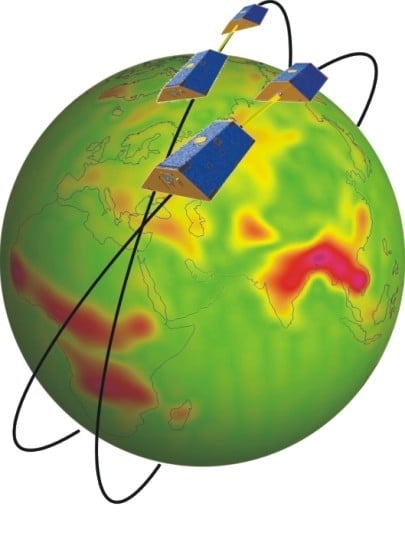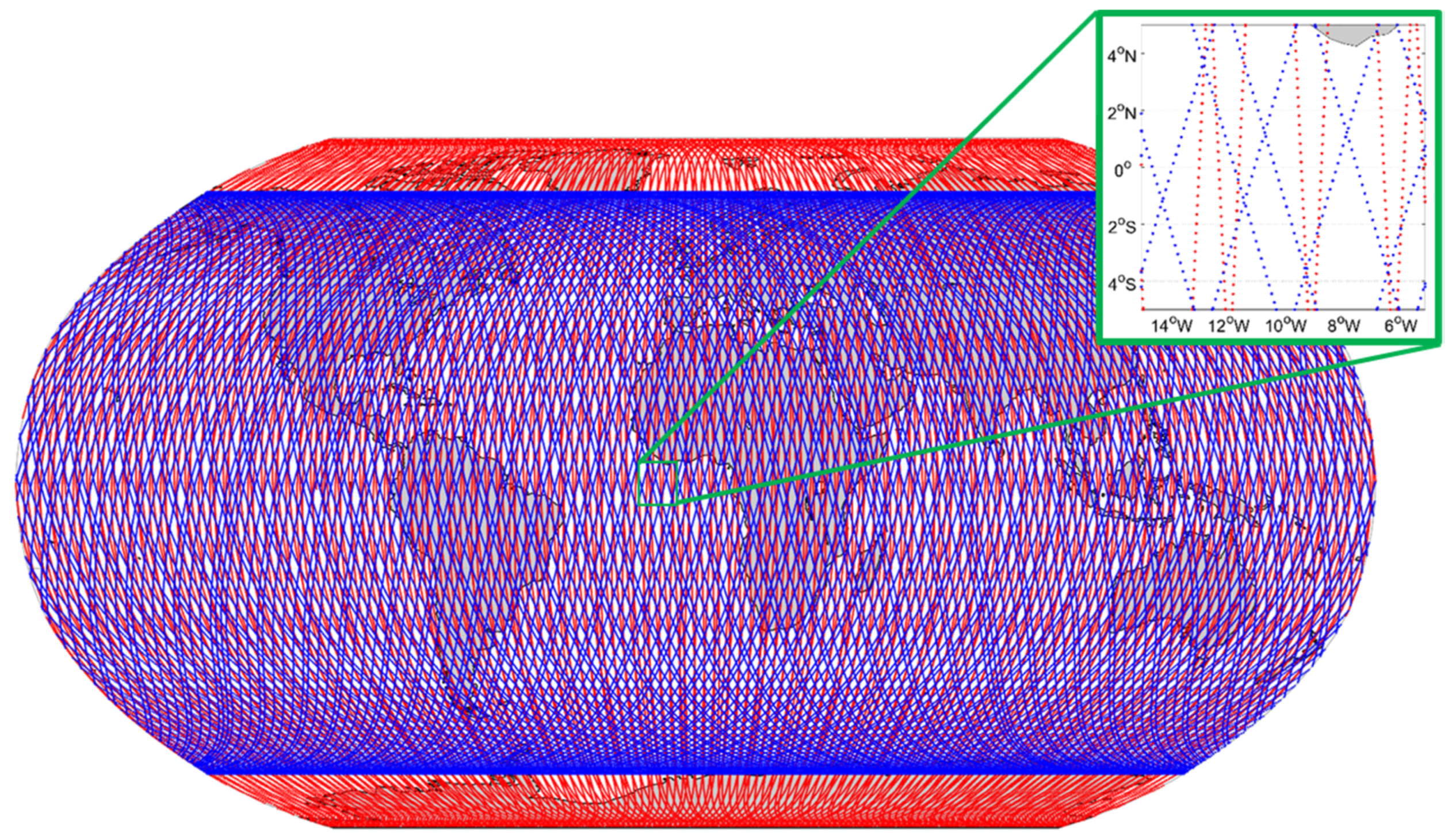Another promising mission scenario is a double-pair constellation being composed of two in-line pairs, the so-called Bender configuration [7]. It is composed of a polar pair similar to the GRACE-type concept, and an inclined pair with an inclination of 65–70 degrees. An example of the resulting ground-track pattern of such a Bender constellation is shown in Figure 1.

Extensive numerical simulations have shown that this set-up also results in a significantly improved isotropy and reduction of stripes, e.g., [8,9], which is mainly due to the different directions of inter-satellite ranging observations, and the different orbital frequencies of the two pairs. Based on this concept, in 2016 e.motion² was proposed as ESA Earth Explorer 9 mission [10]. Another innovative observation concept is high-precision high-low inter-satellite ranging, which was proposed as the MOBILE mission in response to ESA’s Earth Explorer 10 call, e.g., [11] and [12]. On US side, the United States National Academies of Sciences, Engineering, and Medicine published the decadal strategy for Earth observation from space [13], where mass change was identified as one of the top five designated observables to be implemented by future US Earth observation missions, in order to ensure continuity and enable long-term mass budget analyses of the Earth system.

A NGGM concept was also proposed in China, and the key technologies have been developed to meet the requirements of NGGM [14,15,16]. The objectives of Chinese NGGM are not only to perform global gravity measurements, but also to verify the maturity of key technologies required for space-based gravitational-wave detection [17] to a certain level of precision. The scientific objectives and the system requirements of Chinese NGGM are under investigation in these years. This mission is expected to be approved soon, and is planned to launch in the middle 2020s.

The existence of this study roots back to a Round Table China–Europe meeting on Satellite Gravity Exploration, which took place in September 2013 in Beijing. There it was agreed to evaluate options for further joint activities on NGGMs, especially science studies on numerical mission simulations. This was eventually realized in the frame of the European Space Agency’s “Additional Constellation and Scientific Analysis Studies of the Next Generation Gravity Mission (ADDCON)” study. ESA’s ADDCON study team and a Chinese study team joined forces in an initiative to perform numerical studies on NGGMs based on double-pair and multi-pair constellations of GRACE/GRACE-FO-type satellites.

A main prerequisite for the performance assessment and interpretation of joint numerical simulations is to ensure comparability of the results of the contributing groups. Therefore, it was decided early in the project to jointly set up common test scenarios and corresponding data sets, which shall be processed by all contributing processing centers. This paper reports on results of this inter-comparison exercise. The contributing processing centers are Technical University of Munich (TUM), Institute of Geodesy and Geophysics, Chinese Academy of Sciences (IGG-CAS), Tongji University (Tongji), Wuhan University (WHU), and Huazhong University of Science and Technology (HUST).

The paper is structured as follows. Chapter 2 describes the basic idea of a numerical closed-loop NGGM simulation, and describes the main input data, which have been jointly used by all groups. Chapter 3 provides an overview of different methods applied by the study teams. Chapter 4 reports the numerical simulation results, their comparison, assessment, and inter-comparison. The final Chapter 5 contains main conclusions as well as an outlook to future work.

2. Closed-Loop Simulations and Input Data

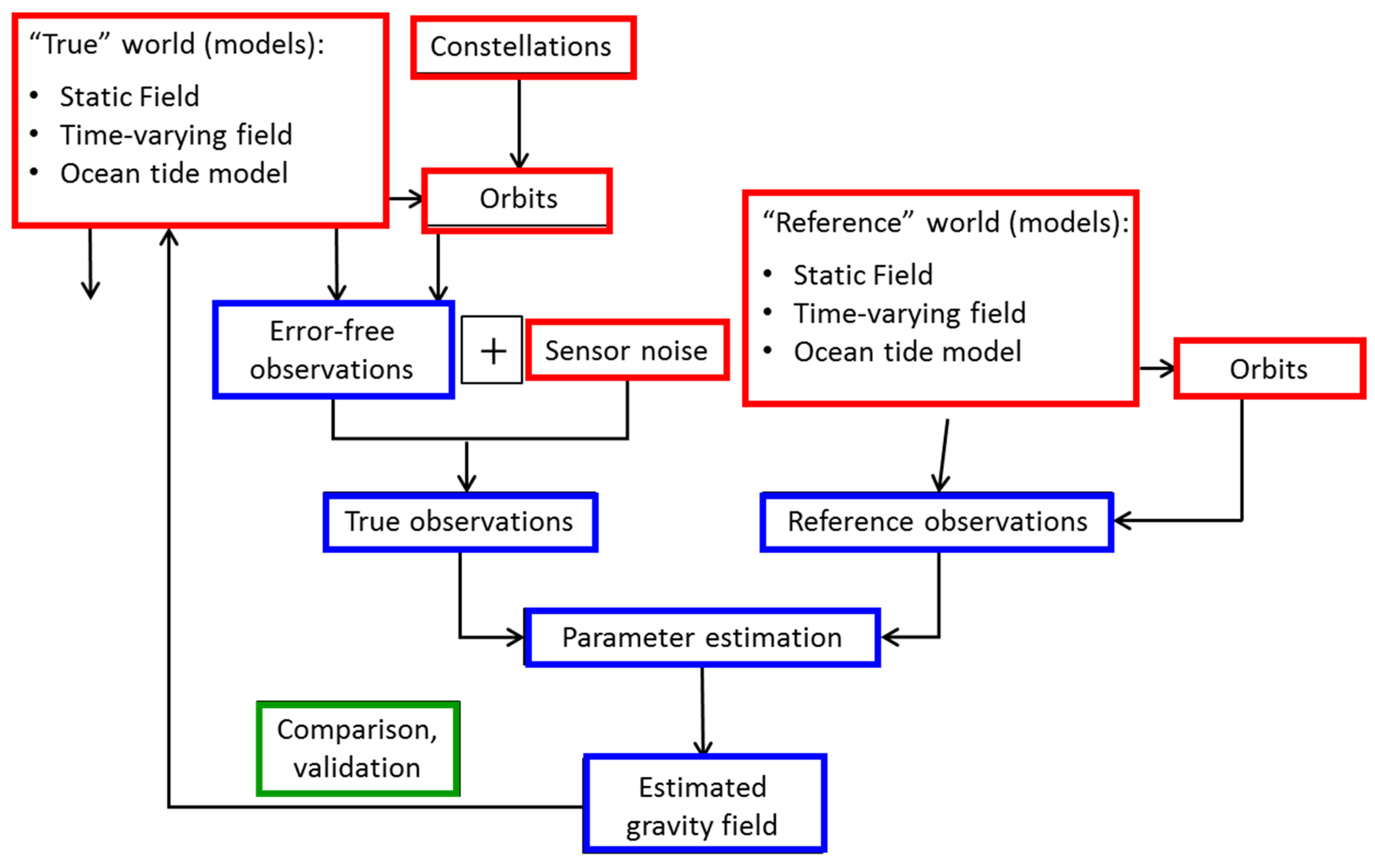
The basis of the inter-comparison exercise are so-called numerical closed-loop simulations. Compared to real-data processing, the advantage of these closed-loop simulations, which are performed in a completely synthetic simulation world, is that the truth is perfectly known. Therefore, the effect of any data set, instrument noise assumption, or processing strategy is directly reflected by deviation of the final result from the “true world”, and can be studied separately from all other error contributors to the total error budget.

Figure 2 shows an overview of the numerical simulation set-up. The simulation starts with the definition of the “true world” (upper left), using force models for the static gravity field as well as tidal and non-tidal temporal variations. All gravity-related models are parameterized as coefficients of a spherical harmonic (SH) series expansion. In parallel, specific orbit constellations and the corresponding orbit parameters have to be defined, in our case Bender-type double pairs. The corresponding orbits are generated by numerical integration. Based on the a-priori force models, error-free observations are computed along the orbit tracks, with a sampling period of 5 s. They are then superimposed by instrument errors with pre-specified spectral noise characteristics, resulting in “true observations”, which mimic as realistically as possible the real observations. On the other hand, a reference world is built up (upper right). This is necessary because the functional model of gravity field estimation from low–low inter-satellite ranging observations is highly non-linear, and this requires a Taylor point as approximate prior knowledge. In the same way as for the “true observations”, so-called “reference observations” are computed, which are based on force models that are usually different from those used for the “true world” scenario. The main goal of the gravity field determination is then to estimate residuals with respect to these a-priori models. Adding the residuals to the a-priori models should result in the ideal case (no errors in the system) in the true world models. In the case that errors do exist, such as instrument errors, but also aliasing errors due to the specific space-time sampling properties of the chosen orbit constellation, the estimated gravity field will deviate from the true world, and thus provides a clear hint on the achievable performance of the specific mission design.

For the inter-comparison exercise, two Bender double-pair scenarios have been defined (

Table 1. Main orbit parameters of numerical simulation scenarios.

Simulation Scenario	Semi-major Axis Minus 6378 km	Inclination (°)	Cycle/Retrieval Period (days)	Start Epoch	Drift Rate (°/cycle)
A	~355/~390	70/89	9	1 Jan 2002	1.5
B	~355/~340	70/89	7	1 Jan 2002	1.3

). They are based on extensive prior studies on optimum orbit design of double-pair configuration with the goal to optimize the space-time sampling. The two scenarios A and B mainly differ in the orbit altitude of the polar satellite (390 vs. 340 km) and their repeat cycle (9 vs. 7 days). The orbits were designed such that ground tracks of the polar and inclined satellite pair drift at the same rate within the sub-cycle period, and (b) the retrieval period is always equal to the length of the sub-cycle, so that the gravity field retrieval is always supported by the densest possible ground track pattern. As a side aspect, these drifting orbits have the additional advantage that they produce a dense ground-track distribution over longer periods of time, which might improve the spatial resolution for the gravity retrieval of long-term static gravity solutions.

Table 2. Force and noise models of the “true” and “reference” world used in the Next Generation Gravity Mission (NGGM) simulations.

Model	True World	Reference World
Static gravity field	GOCO05s [18]	GOCO05s
Non-tidal time-variable gravity field	ESA AOHIS [19]	---
Ocean tides	EOT11a [20]	GOT4.7 [21]
Inter-Satellite Link (ISL) noise	Equation (1)	---
Accelerometer (ACC) noise	Equations (2) and (3)	---
Star tracker (STR) noise	---	---
Orbit noise	1 cm white noise	---

provides an overview of the force and noise models of the true and reference world. Static, tidal, and non-tidal gravity models are used up to SH degree and order (d/o) 120.

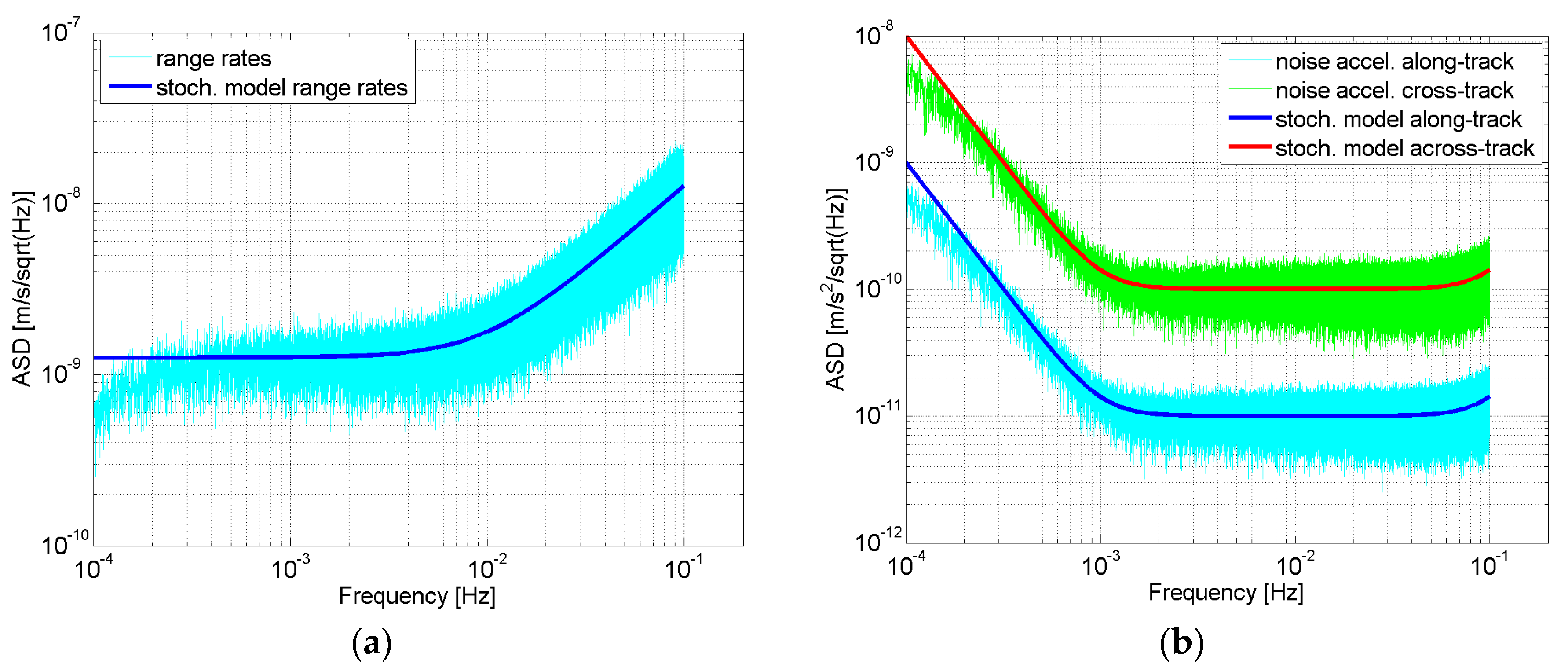
The ISL is assumed to be realized by a Laser Ranging Interferometer (LRI). The assumed spectral noise behavior of the LRI in terms of range rate is expressed by the following Amplitude Spectral Density (ASD) [22]:

$$d_{\mathit{range}\text{-}\mathit{rates}} = 2 \times {10}^{-8} \times 2\pi f \times \sqrt{{\left(\frac{{10}^{-2}\mathrm{Hz}}{f}\right)}^2+ 1}\frac{\mathrm{m}}{\mathrm{s} \sqrt{\mathrm{Hz}}}$$

(1)

where $f$ is the linear frequency. The resulting error spectrum is shown in Figure 3a (dark blue curve), and the corresponding noise realization in light blue color.

The non-gravitational forces are typically sensed by the on-board accelerometers located in the center-of-mass of the satellite. In our simulations, an electrostatic accelerometer is assumed with two high-sensitive axes oriented in the flight direction (largest signal) and radial direction, and one low-sensitive axis in the cross-track direction (see Figure 3b). The accuracy level in terms of accelerations is expressed by [22]:

$$d_{\mathit{acc}. \mathit{along}} = d_{\mathit{acc}. \mathit{radial}} = {10}^{-11}\sqrt{{\left(\frac{{10}^{-3}\mathrm{Hz}}{f}\right)}^4/\left({\left(\frac{{10}^{-5}\mathrm{Hz}}{f}\right)}^4+1\right)+1+{\left(\frac{f}{{10}^{-1}\mathrm{Hz}}\right)}^4}\frac{\mathrm{m}}{{\mathrm{s}}^2\sqrt{\mathrm{Hz}}}$$

(2)

$$d_{\mathit{acc}. \mathit{across}} = 10 \times d_{\mathit{acc}. \mathit{along}},$$

(3)

It has a noise level of 10⁻¹¹ m/s² in the measurement bandwidth, and a $1/f^2$ slope at frequencies from 10⁻³ Hz and lower. Equation (3) expresses the fact that electrostatic accelerometers, as they have been used in all previous and current satellite gravity missions, usually have two high-sensitive axes and one less-sensitive axis. In our set-up, we assume a degraded performance of the less-sensitive axis by one order of magnitude, and that it is oriented in an across-track direction. In this study, we further assume that the attitude, which is usually a minor error contributor compared to ISL and ACC, is known perfectly. Orbit errors are simulated by white noise with a standard deviation of 1 cm. The generation of the ISL and ACC noise time-series was done by scaling the spectrum of normally distributed random time-series with their individual spectral analytical noise model, as given in Equations (1) to (3).

3. Methods

The five contributing processing centers used their specific software systems for NGGM simulation and gravity field recovery. However, as a joint spatial–temporal parametrization, low-degree daily gravity field parameters were co-estimated together with the higher-degree temporal gravity solution, where the latter covers a retrieval period of 9 days (Scenario A) and 7 days (Scenario B). This co-estimation was first proposed by [23] and investigated in detail in [9]. There it could be shown that by this “Wiese parameterization” temporal aliasing can be reduced significantly, because short-term temporal gravity signals (mainly atmosphere and ocean signals), which would alias in standard processing into the solutions, are explicitly estimated, thus avoiding their aliasing effect. On the one hand this “self-dealiasing” approach improves the gravity field solution over the whole spectral range, and on the other hand, as a positive side effect daily gravity field products, which are independent of each other, are produced. This might be an important aspect for operational service applications, where usually a high temporal resolution and short latencies are required [24].

In all five processing centers, the non-tidal gravity field signals along the orbits were derived from the ESA Earth System Model (ESM, [19]) for all five components: atmosphere (A), ocean (O), hydrology (H), ice (I), and solid Earth (S), together abbreviated by AOHIS. Based on the 6-hourly AOHIS input products, the signals at certain measurement epochs were derived by linear interpolation. In the recovery, the full AOHIS signal was estimated, i.e., no a-priori non-tidal de-aliasing is performed, which is possible due to the co-parameterization of daily gravity field parameters [8,9]. Therefore, also no additional errors were assumed for the AOHIS signal. The true world is composed of this AOHIS signal itself, and the reference world does not contain any non-tidal temporal gravity signal (cf. Table 2).

In the following, we describe briefly the different methods applied by the five processing centers. Detailed information can be found in the cited references.

TUM: All simulations were executed with a full-scale numerical mission simulator [25,26], which has already been successfully applied in real data applications to recover satellite-only gravitational field models for CHAMP (Challenging Mini-Satellite Payload), GRACE and GOCE. The simulation environment is based on numerical orbit integration following a multistep method [27], which applies a modified divided difference form of the Adams-Bashforth-Moulton Predict-Evaluate-Correct-Evaluate (PECE) formulas and local extrapolation. The adopted gravity field approach is based on a modification of the integral equation approach from [28] where the orbit is divided into continuous short arcs of 6 h length. The position vectors at the arc node points are set up as unknown parameters, which are estimated together with the gravity field coefficients. As a stochastic observation model, autocovariances computed from an auto-regressive moving average (ARMA) filter model, approximating the spectral characteristics of the residuals of instrument errors, are used [9].

IGG-CAS: Simulation work was done with a full numerical mission simulator, which is modified from the software tool developed in IGG-CAS for recovering satellite-only gravitational field models from GRACE Level1b observations [29]. The simulation environment is based on numerical orbit integration applying the multistep Gauss-Jackson method [30], which uses start-up value using Runge-Kutta single step integral method. The gravity field recovery is based on the variational equation approach or dynamic method, where the orbit is divided into continuous arcs of 6 h length, and initial state vectors at the beginning of the arc are set up as unknown parameters, which are estimated together with the gravity field coefficients. The 1-cpr effect in the residuals of range-rate observation are modelled [31], which are also estimated together with the gravity field coefficients.

Tongji: The simulations were carried out by using the Satellite Gravimetry Analysis Software (SAGAS) developed by Tongji University [32,33,34,35], which has been successfully applied to determine gravity field models from GRACE Level-1b observations. The simulation environment is based on numerical orbit integration, where Adams and Kiogh-Shampine-Gordon (KSG) numerical integration methods are jointly used. The adopted gravity field approach is the modified short-arc approach [32,33,34], where the observation equation is directly linearized with respect to the real orbit observations and the integral arc is divided into continuous short arcs of 2 h in length. Non-conservation acceleration observation errors are estimated together with the gravity field coefficients according to [33,34]. Variance–covariance matrices for both orbit and range-rate observations are constructed from residuals of the instrument errors on the basis of [35].

WHU: WHU team has developed a software platform which was used in the real data processing of the modern satellite gravity missions such as GRACE and GOCE [36,37]. For the current work on the evaluation of the NGGM schemes described in this paper, the brute-force dynamic method was selected as the basic approach in the numerical simulations [38]. For the non-conservative forces there was only accelerometer noise provided, so the orbit was integrated with the non-gravitational forces being constant zeros. In the parameter estimation step, the arc length is adjusted to 1.5 h for an optimal estimation. The initial satellite states of every arc and low degree geo-potential coefficients up to d/o 15 were processed as the local parameters, and the other geopotential coefficients to degree 70 were estimated as the global ones [23]. Regarding the stochastic model, a filtering strategy of processing band-limited measurements proposed by Schuh [39] was applied to deal with the colored observation noise.

HUST: All simulation works were implemented with a full numerical mission simulator, which has been successfully used to develop the HUST gravity field models [40,41]. The simulation environment is based on numerical orbit integration. The Gauss-Jackson multistep method is used for the numerical integration, which applies start-up values using the Runge-Kutta single step integral method. The adopted gravity field approach is based on the variational equation approach or dynamic method. The orbit is divided into continuous arcs of 6 h length, and initial state vectors at the begin epoch are set as unknown parameters, which are estimated together with the gravity field coefficients. Kinematic empirical parameters for range-rates are estimated to reduce the 1-cpr effect in the residuals of range-rate observations. The filtered predetermined strategy (FPS) was applied to process these kinematic empirical parameters [40]. No stochastic observation model was used in this simulation work.

Table 3. Gravity retrieval methods and specific settings of the 5 processing centers.

Proc. Center	Numerical Integration Method	Gravity Retrieval Method	Max. Degree of Input Models	Max. Degree of Retrievals (Subcycle/Daily)	Co-estimated Parameters (in addition to Daily Gravity Fields)	Stochastic Model
TUM	Adams-Bashforth-Moulton (5 s)	Integral equations (short-arc; 6-h arcs)	120	70/15	Initial position and velocity (PV) per arc + boundary condition	Yes, autocovariances based on residuals
IGG-CAS	Gauss Jackson 12 Start: Runge-Kutta-Nyström 12/10	Dynamic method (6-h arcs)	70	Sc.12: 70/15 Sc.13: 65/15	Initial PV per arc	No
Tongji	Adams (5 s) and Kiogh-Shampine-Gordon 7	Integral equations (short-arc; 2-h arcs)	120	70/15	Initial positions, daily polynomials of 5th order, bias and scale parameter for acceleration correction per day	Yes, full covariance based on residuals
WHU	Adams-Bashforth-Moulton (5 s) Start: Runge-Kutta 8	Dynamic method (1.5-h arcs)	120	70/15	Initial PV per arc	Yes, ARMA filter model based on residuals
HUST	Gauss-Jackson 14 Start: Runge-Kutta 8	Dynamic method (6-h arcs)	70	70/15	Initial PV per arc	No

gives an overview of these methods and the specific settings chosen in the gravity retrieval.

All processing centers exploit both orbit data for Global Positioning System (GPS) satellite-to-satellite tracking (SST) in high-low mode, as well as the inter-satellite ranging observations (satellite-to-satellite tracking in low-low mode), by adding the corresponding normal equation (NEQ) systems. No additional constraints such as regularization are applied to the NEQ. As shown in Table 3, the methods mainly differ in the co-estimation of additional parameters and the stochastic modelling of instrument errors. WHU, HUST, and IGG-CAS co-parameterize, in addition to daily gravity parameters, only initial state vectors (orbit positions and velocities) per arc. At TUM, additional boundary conditions between arcs are introduced in order to avoid jumps of consecutive arcs. At Tongji, additional daily parameters (polynomials, bias, scale) are co-estimated.

Table 3 shows that the processing centers have used different maximum degree and order for the computation of the observations (70 vs. 120), but all of them have resolved gravity fields up to d/o 70. However, the spectral leakage effect of the signals beyond d/o 70 is minor compared to the other error sources. If there were a significant spectral leakage effect, it would clearly show up in a severely degraded performance of the very highest resolved degrees [42], which is obviously not the case, as will be shown in Figure 5.

4. Results and Discussions

The simulation scenarios described in Chapter 2 have been processed by all contributing groups applying the methods described in Chapter 3. In this chapter, the results will be compared, assessed, and discussed.

Figure 4 shows the differences of the gravity field solutions of Scenarios A and B to their corresponding references solutions, which are represented by AOHIS mean fields over the 9- and 7-day period, respectively. They are expressed in terms of the degree root mean square (RMS) error of equivalent water heights (EWH), which is computed from fully normalized coefficients of a spherical harmonic series expansion $\left\{{\overline{C}}_{nm},{\overline{S}}_{nm}\right\}$ of degree $n$ and order $m$, by [43]

$${\sigma }_n\left(EWH\right)=\frac{a{\rho }_e}{3{\rho }_w} \frac{2n+1}{1+k_n}\sqrt{{\displaystyle \sum }_{m= 0}^n {\overline{C}}_{nm}^2+ {\overline{S}}_{nm}^2}$$

(4)

where ${\rho }_w$ and ${\rho }_e$ represent the average densities of water and Earth, respectively, $a$ the semi-major axis of the Earth, and $k_n$ the load Love number of degree n. $\left\{{\overline{C}}_{nm},{\overline{S}}_{nm}\right\}$ can either represent the full signal, or the differences between estimated and true coefficients. The EWH expresses the height of a mass-equivalent column of water per unit area. It is used here for comparing the results of five processing centres, because it is one of the standard quantities to express mass change processes in the Earth system, and was also used in the reference document [4] for this purpose. 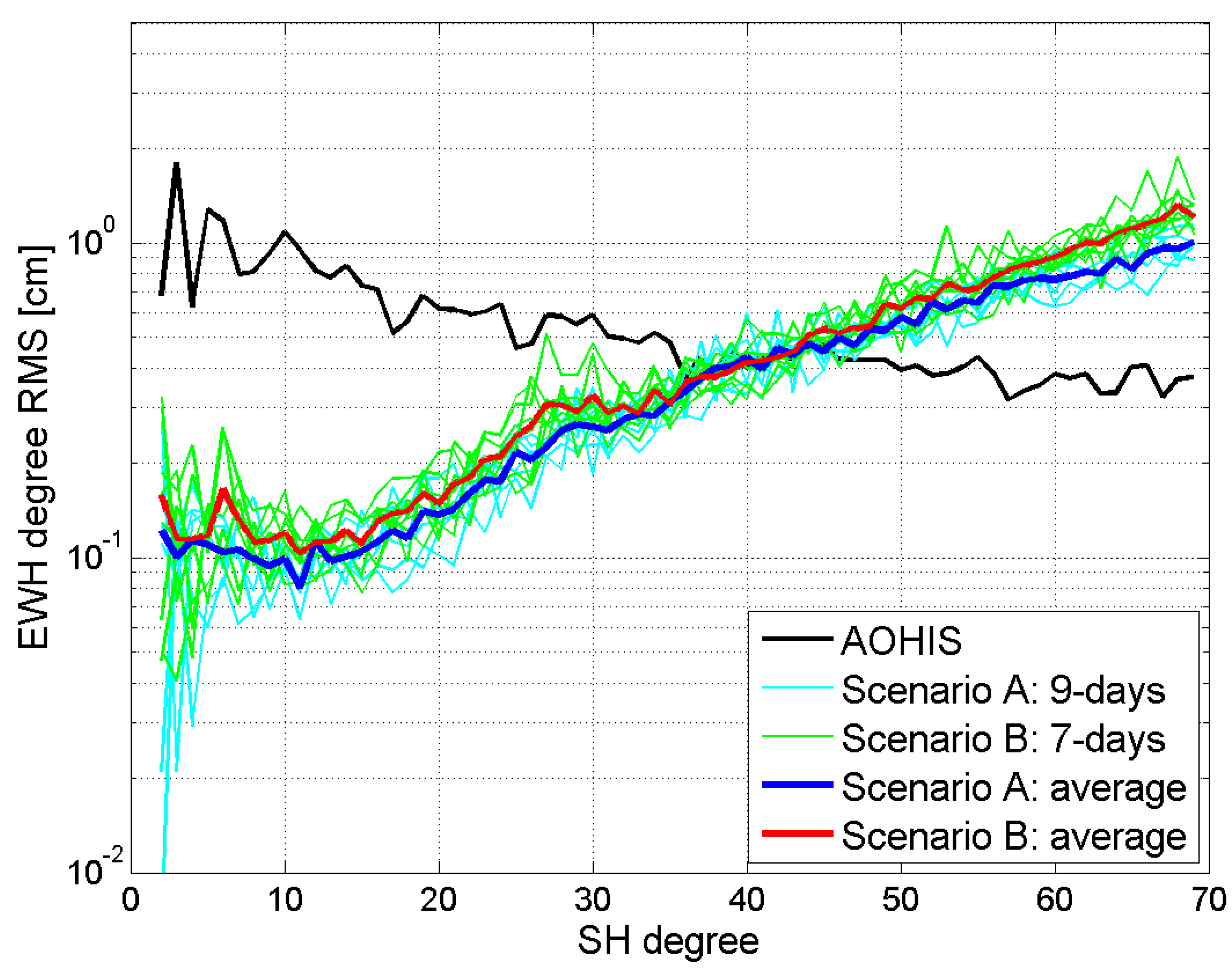Figure 4 shows all 9- and 7-daily solutions obtained by the TUM processor for a two-month period as thin lines, as well as the mean of the two-month period as solid lines. Even though Scenario B is based on an inclined satellite with a lower orbit altitude, the performance of these two scenarios is very similar. This can be explained by the fact that Scenario A comprises 9-day solutions, while in Scenario B the solutions are based only on 7 days each. This lower number of observations seems to counteract the lower orbit altitude of the second pair. Since the performance of these two scenarios is very similar, in the following, when we will inter-compare the solutions of the five processing centers, we will concentrate on Scenario A.

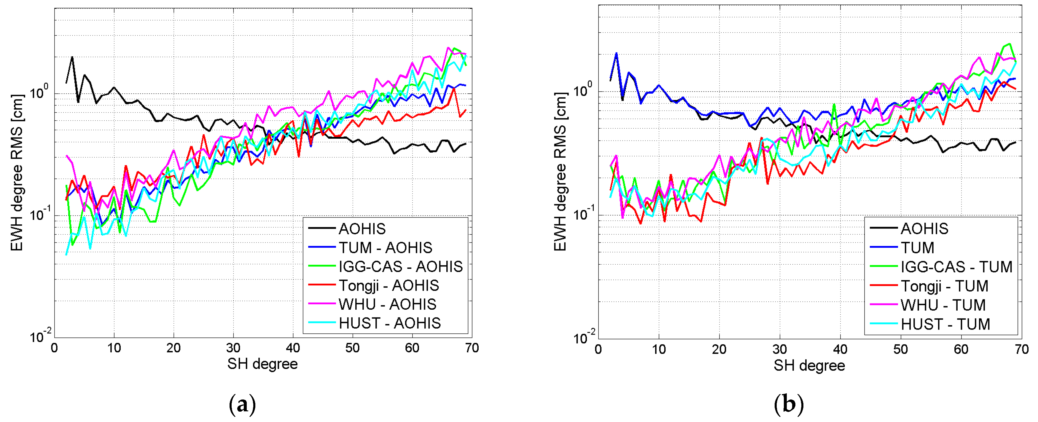
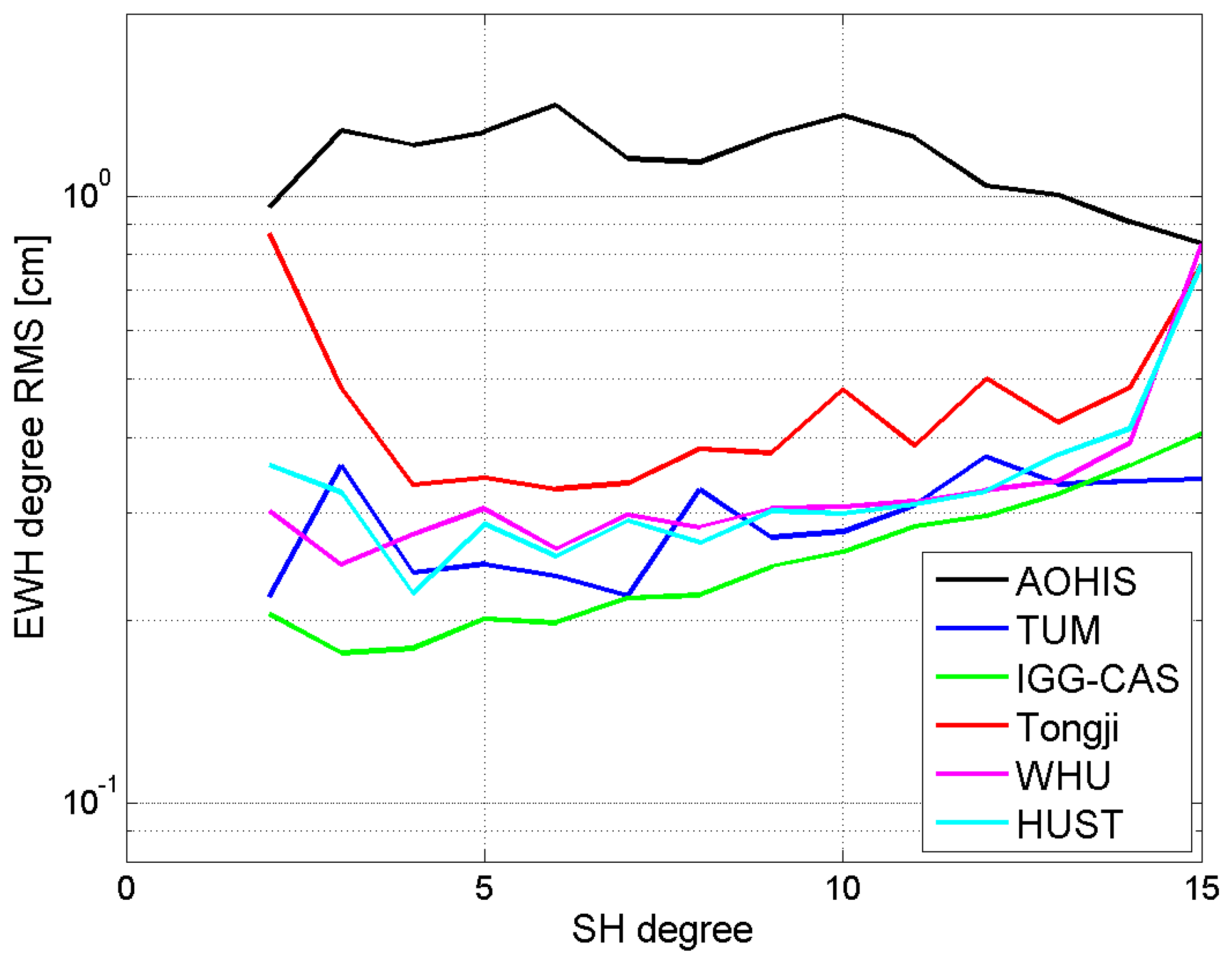
Figure 5a shows the degree RMS of the solutions with respect to the AOHIS input signal of the five processing centers for the first 9-day period. Even though there are several differences, they perform reasonably similarly. Apart from a slightly different error level over the whole SH spectrum, evidently the Tongji solutions perform better in the higher degrees, followed by TUM and WHU. A possible reason could be that both processing centers are using full covariance information as a stochastic model (cf. Table 3). In order to analyze the variability of the solutions among themselves, Figure 5b shows again the degree RMS, but now with the TUM solution as the reference. Evidently, the internal variability of the solutions is almost at the same level as their deviation from the input AOHJS signal.

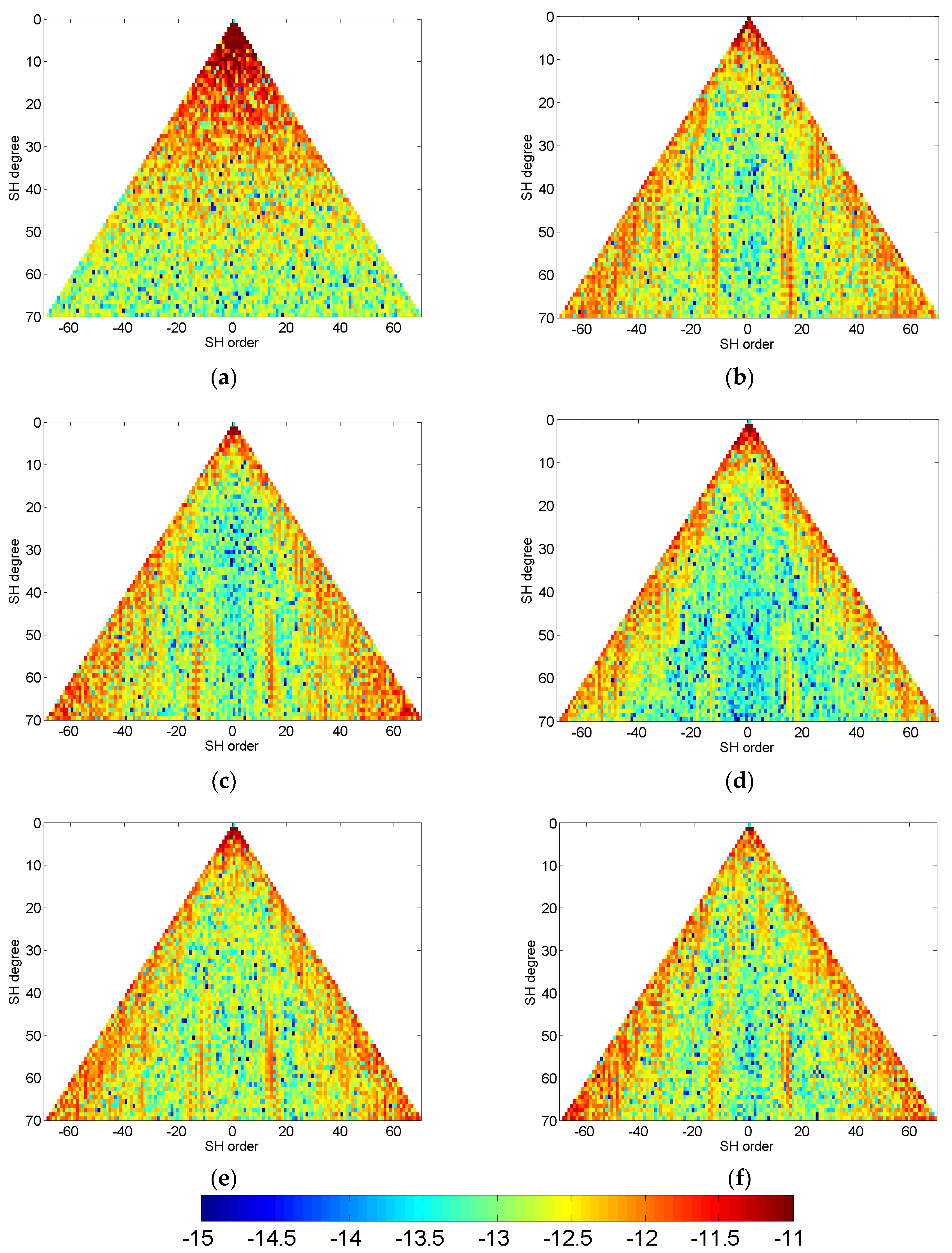
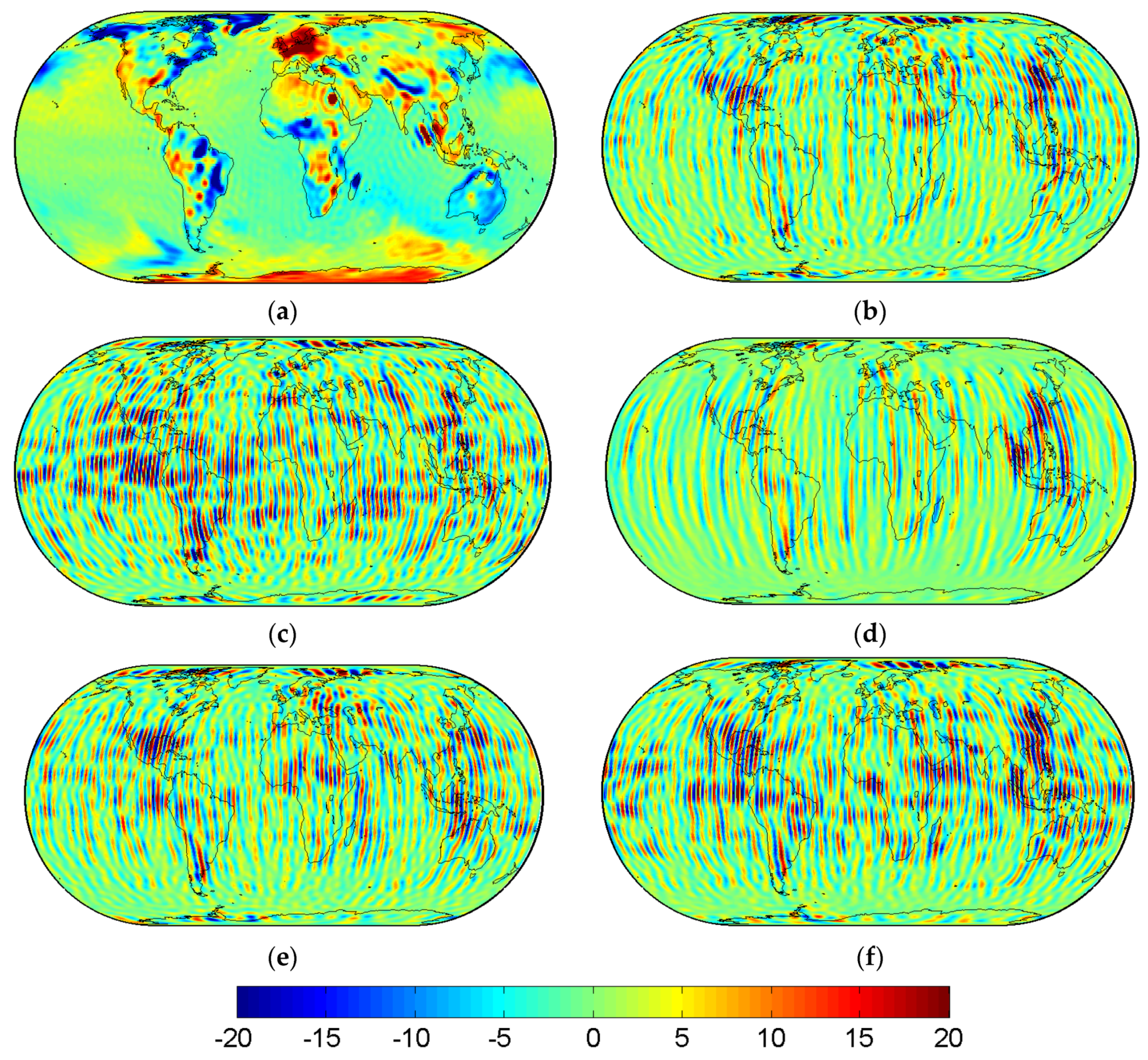
In order to analyze these differences in more detail, Figure 6 shows the SH coefficients of the input AOHIS signal averaged over the first 9 days of the analysis period (Figure 6a), as well as the coefficient differences of the five individual solutions from this AOHIS signal (Figure 6b–f). In general, there is a weakness in the estimation of the sectorial and near-sectorial coefficients, which is intrinsic to the in-line inter-satellite ranging concept. It measures mainly in a North–South direction, while the cross-track direction, which is mainly represented by the sectorial coefficients, is determined worse. 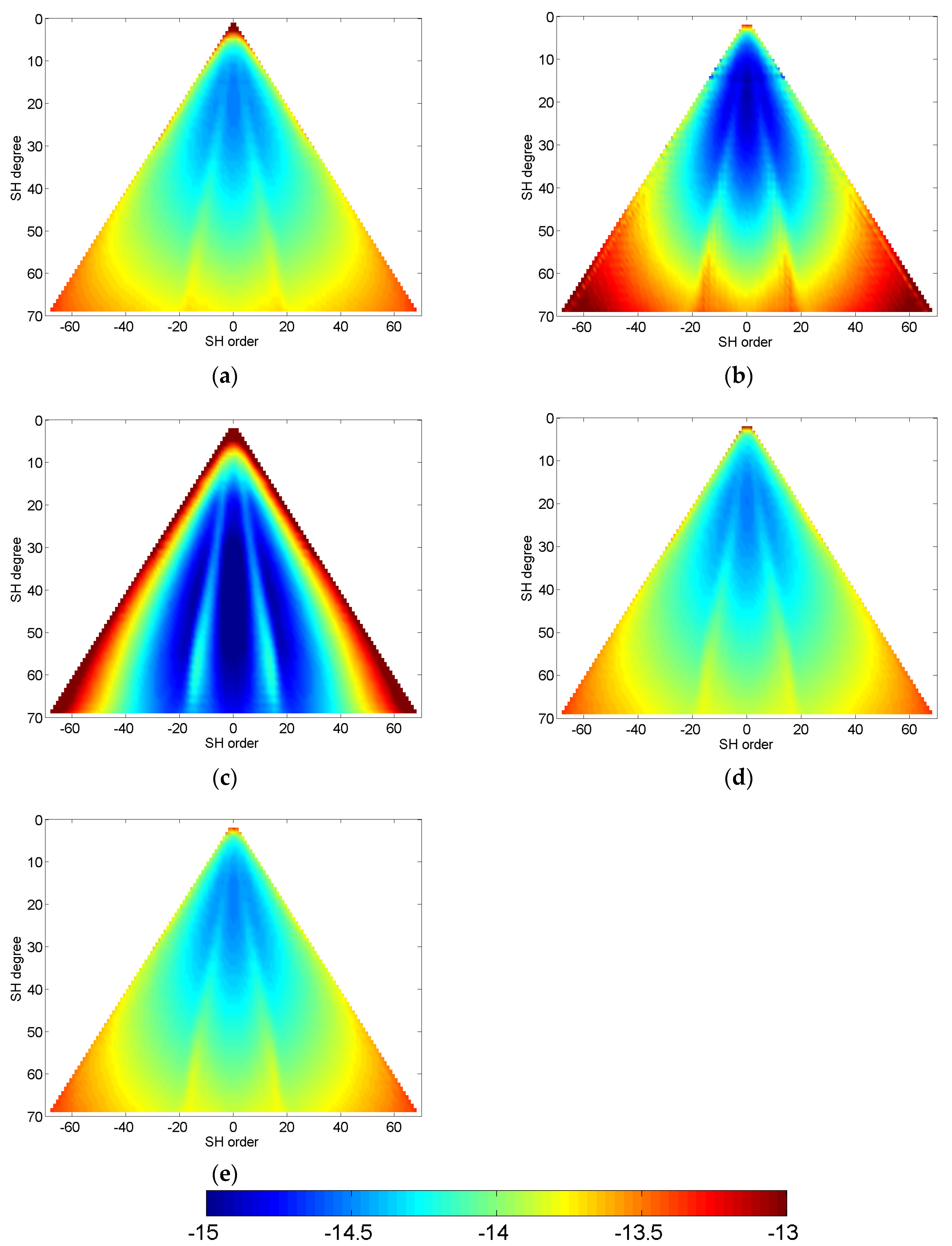This general weakness of in-line pairs is also nicely reflected in the estimated formal coefficient standard deviations (Figure 7), representing the main diagonal elements of the variance–covariance matrix.

A typical feature of Bender-type solutions are the error bands forming an inner triangle, which is directly related to the inclination of the second pair, expressing the fact that the near-polar areas are covered only by observations from the polar satellite pair. Since this feature results from the orbit configuration of the double pair, it is also visible in the estimated error standard deviations (Figure 7). In general, these error standard deviations mainly reflect the observation type, the location of the observations, and the stochastic model of observation errors, but they are blind with respect to signal-related temporal aliasing effects, which affect only the right-hand side of the NEQ system. An exception would be if these systematic effects are included in the stochastic observation model, as it is done in the Tongji solution. Therefore, the coefficient differences to the true solutions (Figure 6) show a higher error level than the formal error estimates and also additional features, because they are affected by temporal aliasing effects.

In Figure 7, the formal error estimates were scaled by empirically derived factors to make them comparable among each other. This was necessary because the processing centers followed different strategies regarding stochastic modelling (cf. Table 3). Of course, in principle the scaling (calibration) of the formal errors could have been done also by means of a-posteriori variance estimates from the post-fit residuals. However, on the one hand this information was not available for all processing centers, and on the other hand these variance estimates would be hampered by the systematic errors related to temporal aliasing effects anyway.

Analyzing the coefficient differences (Figure 6) and the corresponding scaled statistical error estimates (Figure 7) of the various processing centers in more detail, a striking fact is that the triangular error structure related to the Bender-type constellation of the Tongji solution in Figure 6d is much weaker than for the other processing centers, even though it is clearly visible in the error estimate (Figure 7c). This error triangle of the Tongji solution is hardly visible in the coefficient differences to the true AOHIS model of the Tongji solution and looks generally very different from the other solutions (Figure 7c), with much larger degradation of the sectorial and near-sectorial coefficients. As already addressed above, this could be explained by the fact that the covariance information is derived from the post-fit residuals, which contain also temporal aliasing effects. In the IGG-CAS error estimates (Figure 7b), the contrast between the well-estimated near-zonals of lower SH degrees and worse-estimated near-sectorials of high degree is much larger than in the TUM (Figure 7a), WHU (Figure 7d), and HUST (Figure 7e) solutions. Another issue to mention in the error standard deviations is the transition at harmonic degree 15, which is related to the maximum degree of the daily co-parameterization, which is slightly visible in the IGG-CAS formal errors (Figure 7b), while the other four solutions show a very smooth transition. Analyzing the error estimates of the low-degree SH coefficients also reveals significant differences. The error estimates of the IGG-CAS (Figure 7b) and HUST (Figure 7e) solutions predict much lower errors of the low-degree components relative to the high-degree coefficients than the other solutions, which might indicate that the GPS-SST high-low component has been given a higher relative weight when combining the NEQs. In this sense, the analysis of the error estimates allows deeper insights into the gravity recovery strategies, leading, however, as discussed above to very comparable results in terms of SH coefficient retrieval.

Figure 8a shows the global EHW field derived from the full AOHIS signal based on the ESA AOHIS model [19] (cf. Table 2) of the first 9-day period of Scenario A, and Figure 8b–f show EWH difference grids associated to the coefficient differences shown in Figure 6. These global grids have been evaluated up to the full SH resolution of d/o 70. All EWH difference fields show the typical striping pattern which is mainly resulting from residual temporal aliasing. The Tongji and TUM solutions show the lowest stripiness. In order to quantify these results,

Table 4. Main statistical parameters of EWH input and EWH difference fields up to SH d/o 70 of the first 9-day period of Scenario A.

Model (d/o 70)	Min (cm)	Max (cm)	RMS (cm)
AOHIS	−50.38	66.84	5.46
TUM – AOHIS	−37.62	36.69	4.80
IGG-CAS – AOHIS	−29.62	30.43	6.36
Tongji – AOHIS	−31.46	26.71	3.91
WHU – AOHIS	−31.97	32.58	5.41
HUST – AOHIS	−40.68	29.56	6.11

provides an overview of the main statistical parameters of these EWH (difference) fields. Also here, the Tongji solution shows the smallest RMS deviation from the “true” AOHIS model, followed by the TUM result. Evidently, these statistics are dominated by the remaining high-frequency errors expressed by stripes in the EHW fields. Therefore, we re-do the analysis for fields resolved only up to SH d/o 30. According to Figure 5, at this degree the signal-to-noise ratio is safely above one for all five solutions. The results are shown in Figure 9 and

Table 5. Main statistical parameters of EWH input and EWH difference fields up to SH d/o 30 of the first 9-day period of Scenario A.

Model (d/o 30)	Min (cm)	Max (cm)	RMS (cm)
AOHIS	−25.83	24.90	4.74
TUM – AOHIS	−3.63	5.42	0.98
IGG-CAS – AOHIS	−3.14	3.66	0.83
Tongji – AOHIS	−5.46	5.43	1.27
WHU – AOHIS	−3.76	4.55	1.01
HUST – AOHIS	−3.76	4.85	1.02

. Please notice that the scale is reduced from 20 cm to 10 cm for the EWH (difference) fields. In this d/o 30 analysis, now the IGG-CAS solution performs best, followed by the results of TUM, WHU, and HUST. These three solutions are practically on the same error level. This is also consistent with the degree RMS results shown in Figure 5.

As a general conclusion, at degree 30 the RMS variation among the five solutions is in the order of 10% of the total signal RMS. Solutions for other time periods show very similar behavior to the ones presented above, and are therefore not explicitly presented and discussed in this paper.

As already mentioned in Chapter 3, all processing centers co-estimated daily gravity field parameters up to SH d/o 15 in order to reduce temporal aliasing effects. Figure 10 shows the resulting degree error RMS curves, which represent differences of daily estimates to the daily AOHIS “true” signals (black curve), averaged over the whole recovery period. Also here, the performance of these daily solutions are very comparable among the processing centers, where IGG-CAS shows a slightly better performance than TUM, HUST, and WHU, and only the Tongji daily estimates are worse.

5. Conclusions and Outlook

Temporal gravity retrieval results of a future Bender-type double pair mission concept performed by five processing centers of a Sino-European NGGM study team based on jointly defined mission scenarios have been inter-compared and assessed. In spite of some remaining differences, the solutions of the contributing teams TU Munich, Institute of Geodesy and Geophysics, Tongji University, Wuhan University, and Huazhong University of Science and Technology show quite similar performances. In general, these results demonstrate that one of the main goals of this inter-comparison exercise, the consistency of simulation results among the contributing groups, could be achieved to a large extent. Remaining differences might be explained by different processing strategies and partially different parameterizations, such as the co-parameterization of accelerometer biases and drifts, or empirical parameters to compensate for long-wavelength errors in the observation time series. Some remaining differences also exist in the error level of the co-estimated daily solutions.

As already mentioned above, the main study goal was not to identify a “winner” among the contributing groups, but rather to achieve consistency of numerical simulation results of NGGM concepts to the best possible extent, even though five independent software packages, which are based partly on different gravity retrieval methods, have been applied. This positive result is an important pre-requisite and basis for future joint activities towards the realization of NGGMs.

Based on this successful inter-comparison exercise of numerical simulators and in view of the fact that in the future several satellite pairs might be in orbit in parallel, further joint studies on optimized constellations of triple- and multi-pairs will be performed, and their impact on the main fields of applications, such as hydrology, glaciology, and solid Earth physics, will be quantified. The results of these studies will be presented in a follow-up paper.