Infrastructure Safety Oriented Traffic Load Monitoring Using Multi-Sensor and Single Camera for Short and Medium Span Bridges

Abstract

A reliable and accurate monitoring of traffic load is of significance for the operational management and safety assessment of bridges. Traditional weight-in-motion techniques are capable of identifying moving vehicles with satisfactory accuracy and stability, whereas the cost and construction induced issues are inevitable. A recently proposed traffic sensing methodology, combining computer vision techniques and traditional strain based instrumentation, achieves obvious overall improvement for simple traffic scenarios with less passing vehicles, but are enfaced with obstacles in complicated traffic scenarios. Therefore, a traffic monitoring methodology is proposed in this paper with extra focus on complicated traffic scenarios. Rather than a single sensor, a network of strain sensors of a pre-installed bridge structural health monitoring system is used to collect redundant information and hence improve accuracy of identification results. Field tests were performed on a concrete box-girder bridge to investigate the reliability and accuracy of the method in practice. Key parameters such as vehicle weight, velocity, quantity, type and trajectory are effectively identified according to the test results, in spite of the presence of one-by-one and side-by-side vehicles. The proposed methodology is infrastructure safety oriented and preferable for traffic load monitoring of short and medium span bridges with respect to accuracy and cost-effectiveness.

1. Introduction

Over last two decades, bridge structural health monitoring (BSHM) has become a pervasive technique that monitors the static and dynamic bridge responses induced by environmental effects or vehicle loads [1]. As the engineering practice of BSHM develops, an increasing number of structures are now being equipped with data acquisition equipment and sensor network consisting of strain sensors and accelerometers, as well as cameras. The initial purpose of these sensors is normally to observe the behavior of bridge structure over time, and thereby to conduct damage detection and assess the structural condition [2]. Then, with the evolution of related technologies, researchers realized that the collected data may be analyzed to achieve the operational monitoring of the bridges as well, such as capturing the bridge response under extreme loads [3,4,5,6] or monitoring the traffic on the bridge [7,8,9].

For bridge structures, traffic load is the central one among these operational factors. On the one hand, bridges are constructed for traffic purpose. On the other hand, the traffic load might deviate from the original bridge design with the rapid development of the transportation industry. Therefore, monitoring traffic load, including vehicle weight, velocity, quantity, type and trajectory, is crucial for bridge design refinement and safety assessment, as well as operational management. In order to monitor the traffic load of bridges, the bridge weigh-in-motion (BWIM) technique is highlighted [10]. The initial concepts behind BWIM were proposed by Moses [11], who used an instrumented bridge as the weighing scale to estimate vehicle weights in his engineering practice. Due to the advantages in terms of cost efficiency, durability and unbiased accuracy, BWIM technique turns out to be a preferable tool to weigh vehicles and is augmented by many subsequent research and engineering applications [12].

Recognizing the vehicle weight is the motivation of BWIM technique. The identification approach is generally based on the static influence line/surface theory [13]. By now, there have been many engineering practices aimed at recognizing the vehicle weight, yet problems are experienced for obtaining accurate results in complicated traffic cases [14]. The original Moses algorithm used for BWIM purpose has difficulty separating the contribution of the individual vehicles from the bridge response alone when more than one vehicle in adjacent lanes travels side by side on the bridge span. In addition, this method is unable to identify extra traffic information including types, size, axle number and velocity of vehicles, without the help of additional traffic sensors such as radar, road tubes and embedded axle detectors [15]. However, the usage of any sort of those sensors would diminish the advantage of BWIM systems over pavement-based WIM systems.

Fortunately, the bridge structural health monitoring (BSHM) technique might provide solutions. An increasing number of bridges are now being instrumented with sensor network and data acquisition equipment. Through mining the data collected by the BSHM sensor network, extra traffic information might be discovered so as to mitigate the aforementioned problems faced by traditional BWIM techniques. An example is when Yu et al. [16] proposed a BWIM algorithm that was able to identify the lateral position of a single vehicle on a bridge by using seven strain gauges installed transversely at the bottom of the beams. Other valuable attempts use the traffic webcam of a BSHM system to automatically detect the vehicles on bridge and achieve further vehicle information identification [17,18,19,20,21,22,23].

Focusing on the aforementioned key issues of current BWIM techniques, this study combines the strain sensor network and an additional traffic video webcam belonging to a bridge structural health monitoring system, to monitor and identify the traffic load on bridge. The logic of the paper is as follows: i) both the theoretical background and the application procedure of camera visual sensing and strain sensing is introduced; ii) the influence line theory oriented towards gross vehicle weight (GVW) recognition is elaborated on with an emphasis on the multiple-vehicle problem, iii) overall framework of the data integration methodology for traffic monitoring is summarized; iv) field tests on a concrete box-girder bridge are conducted to demonstrate the proposed methodology, especially for complicated traffic cases. The advantages and the potential engineering applications of the methodology are summed up as a conclusion.

2. Traffic Sensing Technologies

2.1. Visual Sensing

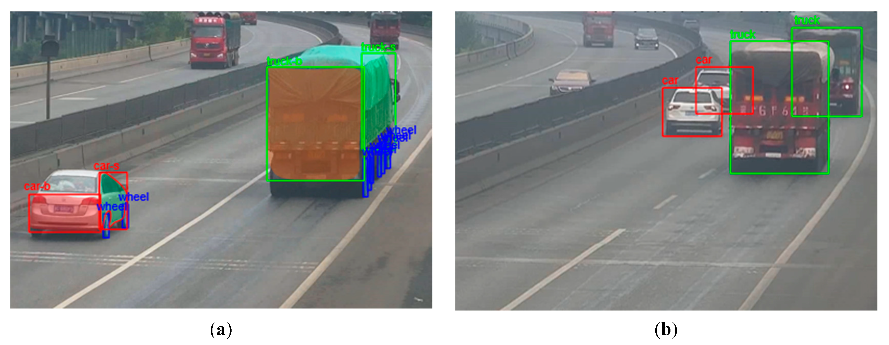
2.1.1. Computer Vision Technique

Over the last decades, the exponential growth in both hardware facilities and software algorithm has successfully made traffic video surveillance widespread. In essence, the goal of traffic video surveillance is the detection of moving object, which aims to decide whether a vehicle exists in the monitored area and where it is. To attain the goal automatically, the computer vision technique is invented, of which the main methods are either motion-based or feature-based. Compared to the motion-based one, the feature-based method is much more efficient and robust due to the upsurge of deep learning, and is considered to be the mainstream of computer vision techniques [24,25].

Convolution neural network (CNN) is a category of neural network with deep structure and convolution calculation. It is one of the representative algorithms of deep learning approaches employed for object detection, classification and segmentation tasks [26]. The learning ability enable the CNN automatically learns features from the training data set, rather than using hand-engineered features, to detect the target object. This process imitates the visual perception mechanism of humans, which makes the CNN leap over the traditional manual feature extraction methods and greatly reduces the workload of operation. The robustness and efficiency of the CNN have been proven in numerous object detection practices.

With the unremitting efforts of computer scientists, superior CNN based computer vision algorithms have been continually proposed. In view of this, an advanced algorithm named Mask Region-based CNN (R-CNN) is applied in this research to detect vehicles in the video surveillance for traffic. The R-CNN is one of the bounding-box object detection approaches. Bounding-box object detection uses a sliding box to search for candidate positions where the object possibly occurs and evaluates the convolutional networks of the image in the box to determine the existence of the object [27]. ‘Mask’ indicates that the Mask R-CNN outperforms the R-CNN by outputting the mask of detected object. Put another way, Mask R-CNN not only detects the existence and position of the objects, but also recognizes the shape of the objects [28].

As with any deep-learning based computer vision algorithm, the implementation procedure of the Mask R-CNN has the following three steps: i) prepare training data sets, ii) train the convolution neural network of the Mask R-CNN algorithm and iii) apply Mask R-CNN to detect vehicles in the traffic video. The real-time detection results in this research are shown in Figure 1.

As seen in Figure 1, the detection tasks of the Mask R-CNN are divided into two trigger strategies: before and after vehicles entering the bridge deck zone. In the first mode, both the back and the side of a vehicle are visible in the video image so that the Mask R-CNN is capable of distinguishing different segments of a vehicle. It is remarkable that the back and side area, as well as closely-spaced wheels of a vehicle are successfully recognized as shown in Figure 1a, proving the segmentation capability of the Mask R-CNN algorithm. When vehicles drive further after entering the bridge deck, the side of the vehicles becomes invisible due to the fixed angle of the camera. Since computer vision techniques cannot detect what is invisible in the image, only the back of vehicles are detected in this scenario, even when the multiple vehicles are overlapping, as shown in Figure 1b.

The image pixel coordinates of the detection box are collected for further size measuring and vehicle positioning tasks.

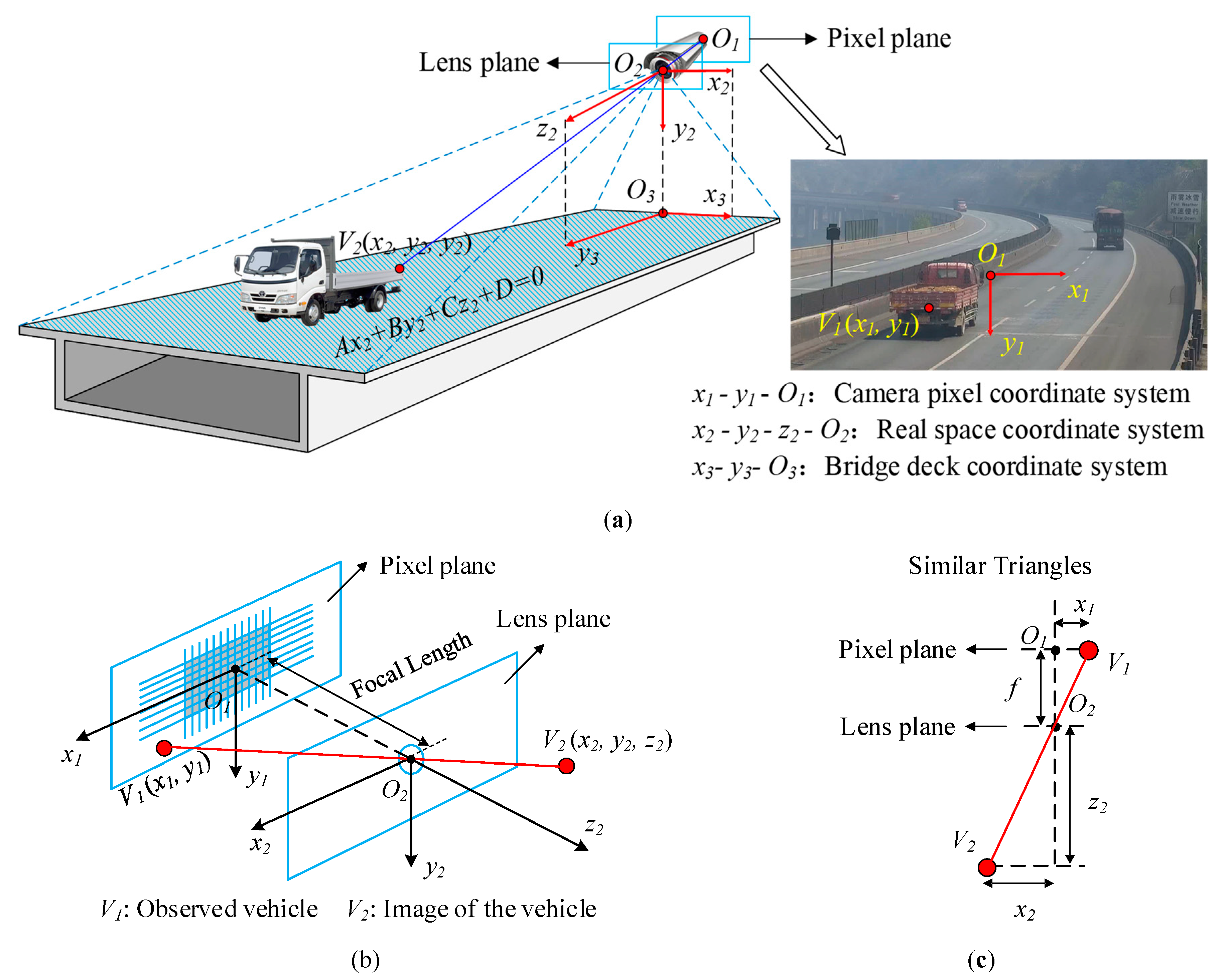
2.1.2. Coordinate Transformation

The raw output of vehicle coordinates from traffic video are in the image coordinate, which cannot be directly used to recognize the velocity, size, or influence value of the vehicles, unless the image coordinates are transformed into the space coordinates. To this purpose, three coordinate systems, namely image pixel coordinate in the video image, space coordinate in the real space, and planar coordinate on the bridge deck, are established for obtaining the vehicle position in situ, as illustrated in Figure 2. A coordinate transformation method is utilized in this paper, basing on the former work of Xu and Zhang [29].

Supposing a vehicle denoted as V is driving on the bridge, what the computer vision technique directly outputs is the pixel coordinate, V₁(x₁, y₁), of the recognized vehicle in the image pixel plane shown in the video image in Figure 2a. In order to get the real space coordinate V₂(x₂, y₂, z₂) of the vehicle, the geometrical relations between the two systems are employed as shown in Figure 2b,c, in which Figure 2c is the planar projection of Figure 2b. According to the geometrical relations, the pixel coordinate of a point V₁(x₁, y₁) can be transferred into spatial coordinate V₂(x₂, y₂, z₂) as follows:

$$\left[\begin{array}{ccc}{x}_1& y_1& f\end{array}\right]\cdot t=\left[\begin{array}{ccc}{x}_2& y_2& z_2\end{array}\right],$$

(1)

where f is the focal length of the camera and t is the similarity coefficient between the two similar triangles in Figure 2c. Now that the coordinate V₁(x₁, y₁) and the focal length f are known, the application of Equation (1) requires to find the similarity coefficient t initially.

Moreover, to get the relative position of vehicles, that is V₃(x₃, y₃), on the bridge deck, it is necessary to firstly consider the bridge deck as a spatial plane in the space coordinate shown in Figure 2. The plane is described by the following equation:

$$A{x}_2+B{y}_2+C{z}_2+D=A{x}_{1}t+B{y}_{1}t+Cft+D=0,$$

(2)

where A, B, C, D are unknown parameters determining the bridge deck plane equation in the spatial coordinate system. The similarity coefficient t can thus be written as:

$$t=\frac{-D}{A{x}_1+B{y}_1+Cf},$$

(3)

The next step is to project the focal point of the camera, i.e., O₂(0,0,0) in Figure 2a, onto the bridge deck plane. As shown in Figure 2a, the projection point is denoted as O₃(x_o3,y_o3,z_o3), of which the coordinates can be easily obtained according to the basic space geometry theory:

$$\left[\begin{array}{ccc}{x}_{o3}& y_{o3}& z_{o3}\end{array}\right]=\left[\begin{array}{ccc}\frac{-AD}{A^2+B^2+C^2}& \frac{-BD}{A^2+B^2+C^2}& \frac{-CD}{A^2+B^2+C^2}\end{array}\right],$$

(4)

Now the coordinate x₃ of the vehicle in the bridge deck coordinate system can be obtained through calculating the distance between the vehicle point V₂(x₂, y₂, z₂) and the plane z₂O₂O₃ in the real space coordinate system shown in Figure 2a above. Assuming the plane z₂O₂O₃ is determined by two coplanar vectors, $\overrightarrow{O_2{O}_3}=\left[\begin{array}{ccc}{x}_{o3}& y_{o3}& z_{o3}\end{array}\right]$ and $\overrightarrow{O_2{z}_2}=\left[\begin{array}{ccc}0& 0& 1\end{array}\right]$, then the coordinate x₃ is expressed as:

$$\{\begin{array}{l}\left[\begin{array}{ccc}{A}_x& B_x& C_x\end{array}\right]=\overrightarrow{O_2{O}_3}\times \overrightarrow{O_2{z}_2}\\ x_3=\frac{A_x{x}_2+B_x{y}_2+C_x{z}_2}{\sqrt{A_x{}^2+B_x{}^2+C_x{}^2}}\end{array},$$

(5)

where A_x, B_x and C_x are the coordinates of the normal vector belong to the spatial plane z₂O₂O₃.

Similarly, the coordinate y₃ of the vehicle in the bridge deck coordinate system can be obtained through calculating the distance between the vehicle point V₂(x₂, y₂, z₂) and the plane x₂O₂O₃. The expression is:

$$\{\begin{array}{l}\left[\begin{array}{ccc}{A}_y& B_y& C_y\end{array}\right]=\overrightarrow{O_2{O}_3}\times \overrightarrow{O_2{x}_2}\\ y_3=\frac{A_y{x}_2+B_y{y}_2+C_y{z}_2}{\sqrt{A_y{}^2+B_y{}^2+C_y{}^2}}\end{array},$$

(6)

The coordinates V₃(x₃, y₃) exactly describe the vehicle position on the bridge deck and will be directly used for BWIM purpose. Noticing that the camera orientation is not always identical with the bridge longitudinal direction due to the limited installation position of the camera, simple coordinate shift and rotation are needed in such cases.

Finally, the key issue of the coordinate transformation turns out to be the determination of parameters A, B, C and D. Instinctively, both the location and orientation of the webcam are needed for parameters determination. However, these data are generally unavailable because of some field conditions. For this reason, a new method is proposed in the companion paper [30], which obtains essential parameters directly from the video image with simply two lines of equal space length in the image regardless of the camera location and/or its orientation. For the conciseness of this paper, that method is not elaborated herein.

2.2. Bridge Strain Sensing

BWIM techniques generally take advantage of the bridge strains to recognize the gross vehicle weight (GVW) based on the static influence line theory. Unfortunately, the raw strain data collected by strain sensors contains the strain induced not only by vehicle weight, but also by vehicle-bridge couple vibration and other environmental factors. Therefore, analyzing bridge structural strain and conducting strain signal processing are imperative. Typically, the components of bridge strain can be denoted as the follow equations:

$${\epsilon }_{bridge}={\epsilon }_{environment}+{\epsilon }_{vehicle},$$

(7)

$${\epsilon }_{vehicle}={\epsilon }_{dynamic}+{\epsilon }_{static},$$

(8)

where ε_bridge is the bridge strain measured from sensors; ε_environment is the bridge strain caused by environmental factors; ε_vehicle is the bridge strain induced by vehicles, which consists of dynamic ε_dynamic and static ε_static components.

Within the different conponents of strains, the static component ε_static is the one needed for the GVW estimation according to the influence theory, and it can be extracted from the measured ε_bridge by filtering ε_environment and ε_dynamic. Technically, a local regression algorithm named locally weighted scatterplot smoothing (LOWESS) is used to realize the extraction approach in time domain. This algorithm is chosen due to its accuracy and convenience, according to Cleveland and Devlin [31]. The whole procedure is shown in Figure 3 for illustration. Details of implementation are available in the literature [30].

It is noteworthy that the above discussion is merely applicable for short and medium span bridges that are commonly chosen as the targets of BWIM implementation [32]. In contrast to long-span bridges, short and medium span bridges serve as ideal weighing scales to estimate the GVW for their structural simplicity, better linear elasticity and more observable responses under traffic loads. Furthermore, environmental load effects on those bridges, such as wind load, are relatively simple or even negligible.

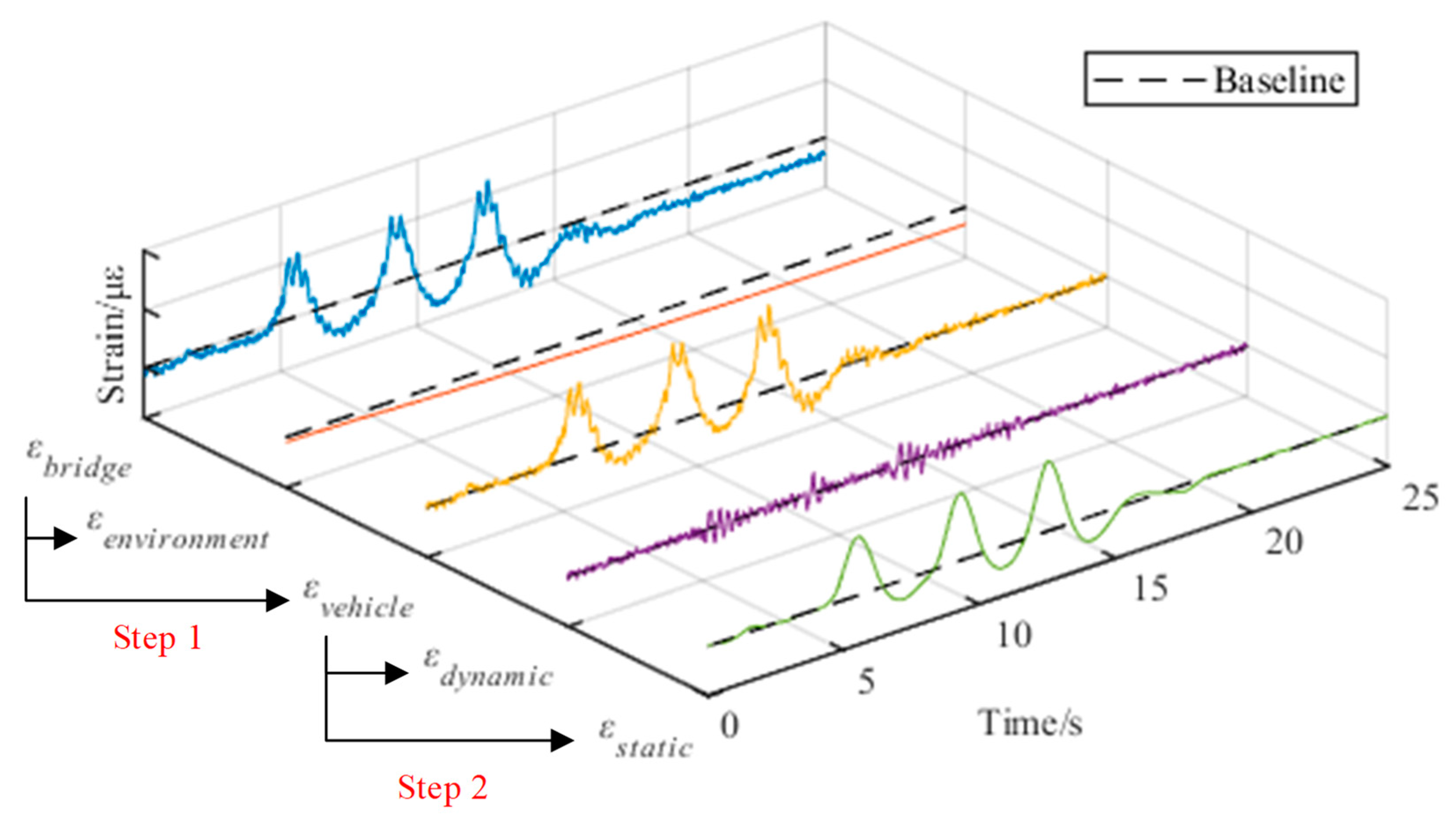
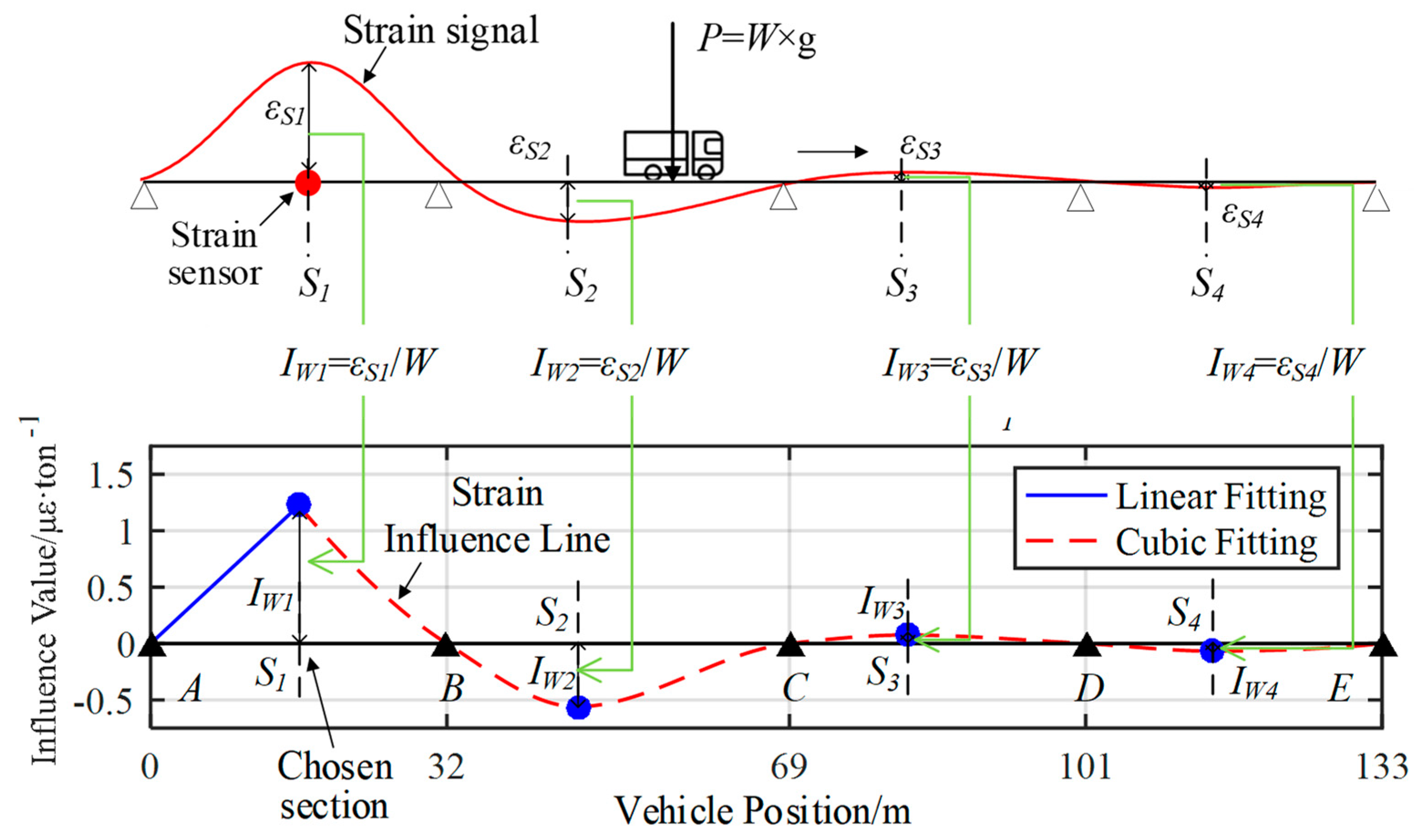
3. Traffic Load Identification with Redundant Measurements

3.1. Traffic Load and Bridge Reaction

As bridges are basically beam-like structures, the influence lines of bridges reflect the relationship between structural responses and traffic load. Available studies regarding BWIM suggest two approaches to obtain the influence line of a bridge, e.g., theoretical derivation based approach [11,33,34] and field tests based calibration [35,36].

This paper employs a method fitting strain influence line with measured strain data from field calibration tests. The method includes two steps [30]: first, the shape of the strain influence line of the target bridge is theoretically obtained with the kinematic method according to Timoshenko and Young [37]; second, a truck with known weight is arranged to cross the instrumented bridge several times as the calibration tests. The strain data measured in the tests is used to determine the exact value of the influence line obtained in the first step. The truck load is simplified as a concentrated load P = Wg for the sake of calibration convenience, where ‘W’ is the vehicle weight and ‘g’ is the gravitational acceleration of which the numerical value is 9.8 m/s². The simplification is reasonable in mechanics, since for the linear elastic structures, the superposition principle works. The accuracy of the GVW recognition results in this paper also supports the simplification. Figure 4 demonstrates the procedure of obtaining the influence line of a four-span continuous bridge for BWIM purpose.

3.2. Identification with Irredundant Measurement

Now that the static component of the vehicle induced strain and the calibrated strain influence line are obtained, the inverse influence line theory can thereby be used to calculate the GVW. According to Timoshenko and Young [37], the influence line theory is expressed as:

$$\epsilon ={\displaystyle \sum _{i=1}^N{W}_i\cdot I_{Wi}}\left(x_i\right),$$

(9)

where ε is the value of the extracted static bridge strain, N is the total number of vehicles on the bridge and W_i, I_Wi(x_i) and x_i are the GVW, the strain influence value and the position of the ith vehicle when the extracted strain signal reaches the local peak, respectively.

Equation (9) can also be written in matrix form as follows:

$$\epsilon =W·I=\left[\begin{array}{cccc}{W}_1& W_2& \cdots & W_N\end{array}\right]·{\left[\begin{array}{cccc}{I}_{W1}\left(x_1\right)& I_{W2}\left(x_2\right)& \cdots & I_{WN}\left(x_N\right)\end{array}\right]}^T,$$

(10)

Since the motivation for BWIM research is to identify the vehicle weight, Equation (10) is supposed to be used inversely to calculate the W. In case of only one vehicle driving on the bridge, Equation (10) can be expressed as:

$$\epsilon =W_1\cdot I_{W1}\left(x_1\right),$$

(11)

Then, using strain data collected by a single strain sensor is enough to determine the GVW of that vehicle. The sole GVW can be easily calculated by:

$$W=\frac{{\epsilon }^{peak}}{I^{peak}},$$

(12)

where ε^peak is the peak value of vehicle induced static strain, I^peak is the peak value of the calibrated strain influence line and W is the GVW of the vehicle. For a more intuitive illustration, ε^peak and I^peak correspond to the ε_S1 and I_W1 in the Figure 4 above, respectively.

3.3. Least Square Based Identification with Redundant Measurements

More generally, there are multiple vehicles driving on the bridge at the same time. In this multiple-vehicle scenario, no determined solution of the W in Equation (10) can be found, unless redundant measurements from multiple strain sensors are available. If strain sensors outnumber the vehicles, which is usually the case, Equation (10) is the form below.

$$\epsilon =\left[\begin{array}{cccc}{\epsilon }_1& {\epsilon }_2& \cdots & {\epsilon }_M\end{array}\right]=W·I=\left[\begin{array}{cccc}{W}_1& W_2& \cdots & W_N\end{array}\right]·{\left[\begin{array}{cccc}{I}_{W1}^{\epsilon 1}\left(x_1\right)& I_{W1}^{\epsilon 2}\left(x_1\right)& \cdots & I_{W1}^{\epsilon M}\left(x_1\right)\\ I_{W2}^{\epsilon 1}\left(x_2\right)& I_{W2}^{\epsilon 2}\left(x_2\right)& \cdots & I_{W2}^{\epsilon M}\left(x_2\right)\\ ⋮& ⋮& \ddots & ⋮\\ I_{WN}^{\epsilon 1}\left(x_N\right)& I_{WN}^{\epsilon 2}\left(x_N\right)& \cdots & I_{WN}^{\epsilon M}\left(x_N\right)\end{array}\right]}_{N\times M},$$

(13)

where ε_N is the maximum strain data collected by the Nth strain sensor, $I_{WN}^{\epsilon M}\left(x_N\right)$ is the Nth vehicle’s influence value belonging to the Mth strain sensor (M > N) and x_N is the position of the Nth vehicle when the bridge strain reaches the maximum. Based on Equation (13), the inverse influence line equation aiming at determining the GVW of multiple vehicles is written as:

$$W=\epsilon ·I^{\mathrm{g}}=\left[\begin{array}{cccc}{\epsilon }_1& {\epsilon }_2& \cdots & {\epsilon }_M\end{array}\right]·{\left[\begin{array}{cccc}{I}_{W1}^{\epsilon 1}\left(x_1\right)& I_{W1}^{\epsilon 2}\left(x_1\right)& \cdots & I_{W1}^{\epsilon M}\left(x_1\right)\\ I_{W2}^{\epsilon 1}\left(x_2\right)& I_{W2}^{\epsilon 2}\left(x_2\right)& \cdots & I_{W2}^{\epsilon M}\left(x_2\right)\\ ⋮& ⋮& \ddots & ⋮\\ I_{WN}^{\epsilon 1}\left(x_N\right)& I_{WN}^{\epsilon 2}\left(x_N\right)& \cdots & I_{WN}^{\epsilon M}\left(x_N\right)\end{array}\right]}^{\mathrm{g}},$$

(14)

It is noteworthy that the influence value matrix I is not a square matrix, which means it only has a pseudo inverse instead of a regular inverse. The pseudo inverse of I is denoted as I^g, satisfying II^gI = I.

The influence value I(x) of the vehicles is unknown without the position information, x, of the vehicles. Vehicles do not always simultaneously pass the bridge cross-section where I reaches its maximum; hence, Equation (12) is ineffective in the multiple vehicles situation. Such is the reason why identifying the presence of multiple-vehicle is still one of the main challenges faced by BWIM technology, as Yu et al. [16] stated. Fortunately, in this paper, the position of vehicles can be quantitatively identified by the deep learning based computer vision technique, which means that the influence values of every vehicle driving on bridge in every moment are available. The multiple-vehicle problem is thus solved.

In addition, Equation (14) is overdetermined, as the equations outnumber the unknowns (M > N). The redundant information in the overdetermined equation helps to reduce the GVW recognition error caused by inaccurate vehicle position or influence line calibration.

An overdetermined equation, however, gives no exact solutions based on matrix algebra. According to Lawson and Hanson [38], the method of ordinary least squares can be used to find an approximate solution to the overdetermined systems. For the equation ε = WI, the least squares formula is obtained from the problem:

$$\underset{W}{\min }\Vert WI-\epsilon \Vert ,$$

(15)

The solution of which can be written in the normal equation:

$$W={\left(I^{T}I\right)}^{-1}{I}^T\epsilon ,$$

(16)

Then, the GVW results, W, are successfully calculated with better accuracy. It is noteworthy that the approach solving the overdetermined equation is effective for both one-vehicle and multiple-vehicle scenario, which helps to reduce the complexity of calculating the GVW in engineering practice.

Furthermore, considering the fact that GVW recognition results of different strain sensors might have different accuracy, the weighted least square method is adopted to reduce the error caused by singular values. Expression of the method is denoted as:

$$W={\left(I^{T}wI\right)}^{-1}{I}^{T}w\epsilon ,$$

(17)

where w is the diagonal weight matrix and can be calculated using w_ii = 1/σ_i², in which σ_i is the variance of the GVW recognition results of the ith sensor.

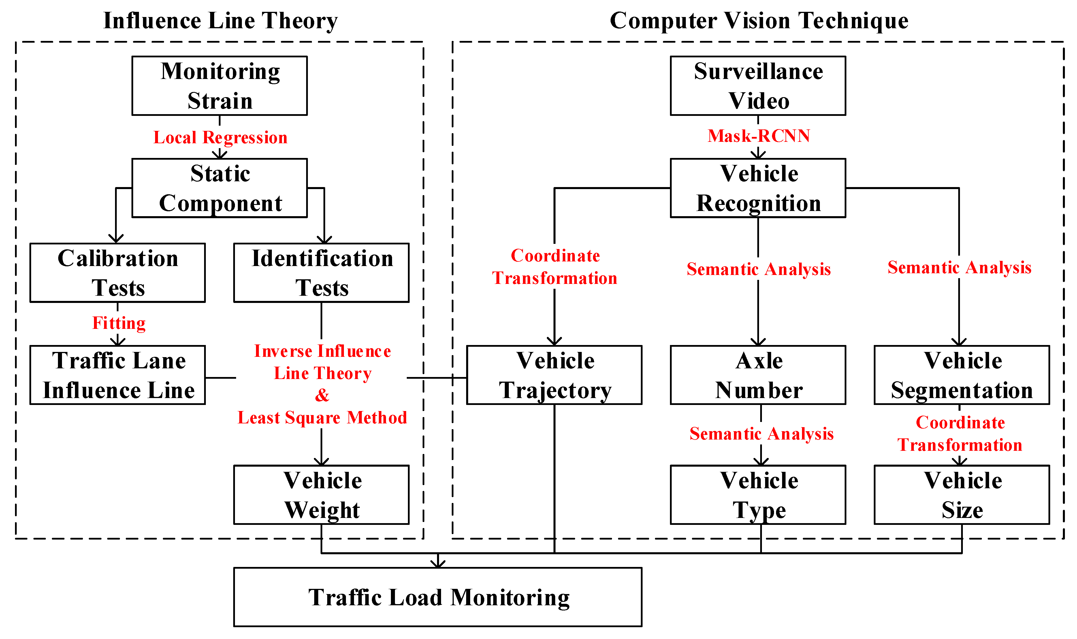
4. Traffic Load Monitoring Framework

Combining the two sensing techniques presented above, the overall data integration framework proposed in this paper can be described as follows.

In the part of strain sensing, since the influence theory is a static mechanics concept, a local regression algorithm named LOWESS is used to extract the static component from the dynamic bridge strain response induced by vehicles. Then, calibration field tests are conducted to obtain the traffic lane influence line of the target bridge with the static strain induced by vehicles.

In the part of visual sensing, after its training, the Mask-RCNN algorithm is used to recognize vehicles in every video frame and pick up vehicle information such as position, type and size etc.

Finally, by combining the calibrated influence line, the obtained static bridge strain and the vehicle position, gross vehicle weight (GVW) can be calculated regardless of the presence of multiple vehicles. The whole procedure is summarized in Figure 5.

It is worth mentioning that the vehicle type and size does not reflect the vehicle weight recognition tasks in this paper, but they are closely noticed by the traffic and bridge management department. For example, oversized trucks are often prohibited from driving on some bridges; therefore, recognizing the type and size of such vehicles and sounding an alarm automatically are of significance in this case. As for how to achieve this recognition, the vehicle type can be directly output by the Mask R-CNN because of the feature-based advantage. The vehicle size, namely the length, width and height of the vehicle, can be recognized through coordinate transformation after the back and the side of the vehicle are segmented. Since this paper mainly focuses on estimating the vehicle weight in multiple-vehicle scenarios, more details about the size recognition are omitted for the conciseness.

5. Field Tests Validation

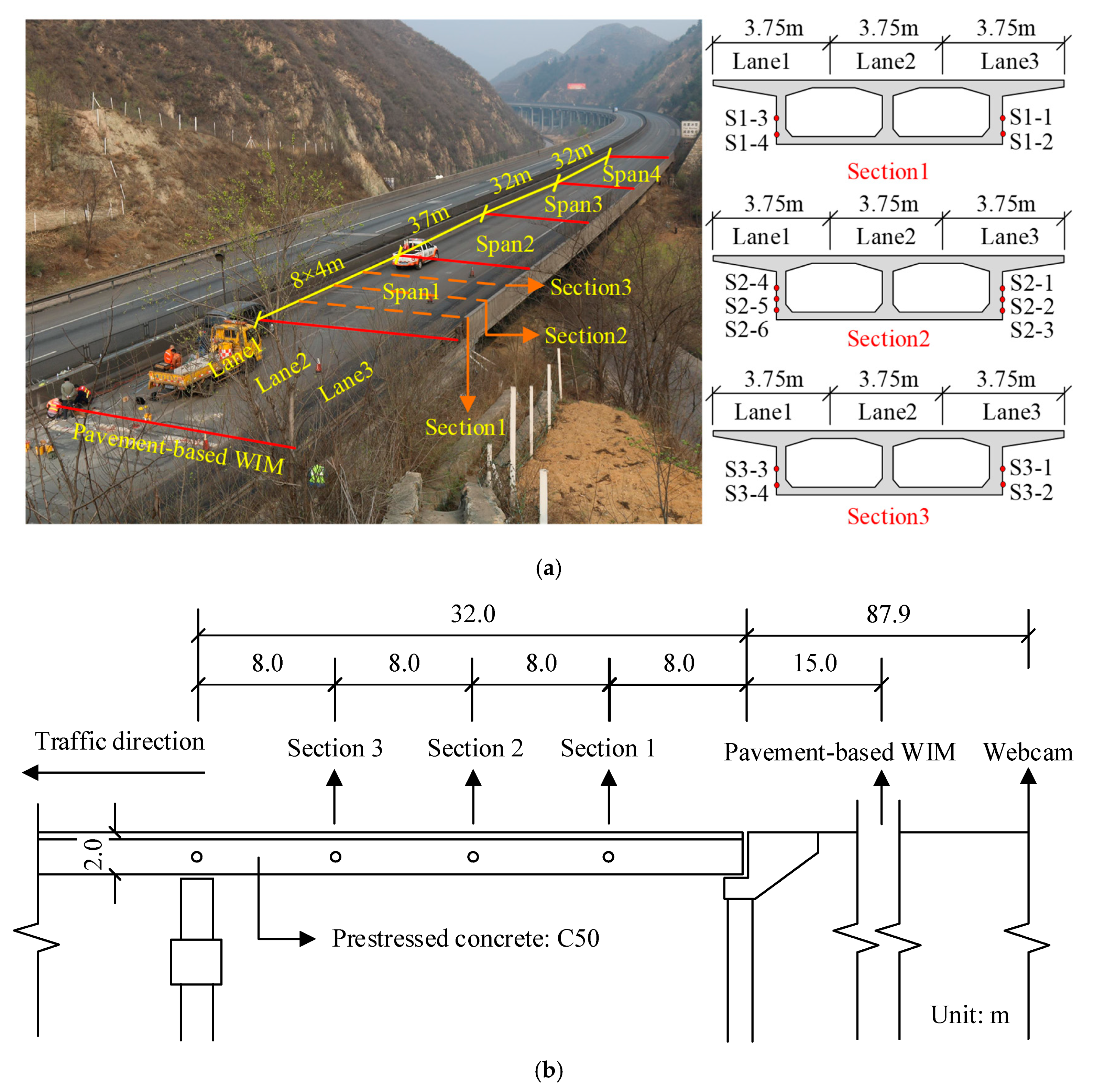
5.1. Instrumentation and Test Setup

Field tests were conducted on an existing bridge for the verification of the proposed traffic monitoring methodology. The tested bridge, referred as Fuchang Overpass (Figure 6), is located on the Baoding-Fuping Highway in Hebei province, China. It is a typical prestressed continuous girder bridge which has been in operation for many years, with a total length of 133 m (32 m + 37 m + 32 m + 32 m). The bridge consists of three traffic lanes in total, and each of them is 3.75 m wide. Lane 3, as the emergency lane, was ignored in this research, since vehicles are prohibited to drive on this lane under normal conditions. The first span of the bridge is instrumented with a structural health monitoring (SHM) system comprising of a pavement-based WIM system, 14 resistance-type strain sensors (named ‘S1-1’ ~ ‘S3-4’) and a webcam. The SHM system was installed with many kinds of sensors (strain gauge, thermometer, accelerometer etc.) for general monitoring purpose, but only strain sensors were employed in this research. The normal strain data in the field tests were recorded by the strain sensor network placed on three different cross-sections, i.e., at 1/4, 1/2 and 3/4 spans and numbered as Section 1, Section 2 and Section 3, respectively. All the discussed information is shown in Figure 6.

The acquired strain data and the video are stored in an online server for long-term and online monitoring of the bridge structure. As a contrast, vehicle weight and velocity measured by a pavement-based WIM system are used as a standard to evaluate the accuracy of this proposed methodology. In addition to all the foregoing, influence lines of traffic lane 1 and lane 2 of bridge structure are obtained in the field calibration tests according to the aforementioned procedure in Section 3.1. Figure 7 illustrates the calibrated influence line on two traffic lanes of all 14 strain sensors on instrumented bridge cross-sections 1, 2 and 3. The vertical axes of the influence line plots are the influence value (IV, unit: με/ton). The calibrated influence lines directly reveal the quantitative relationship between the GVW and the strain data collected by different strain sensors. As the influence lines significantly outnumber the vehicles driving on the bridge and each of the lines is different, they also deliver the deployment foundation for the GVW recognition algorithm using redundant measurements. Otherwise, it is needless to calibrate the influence lines of multiple strain sensors.

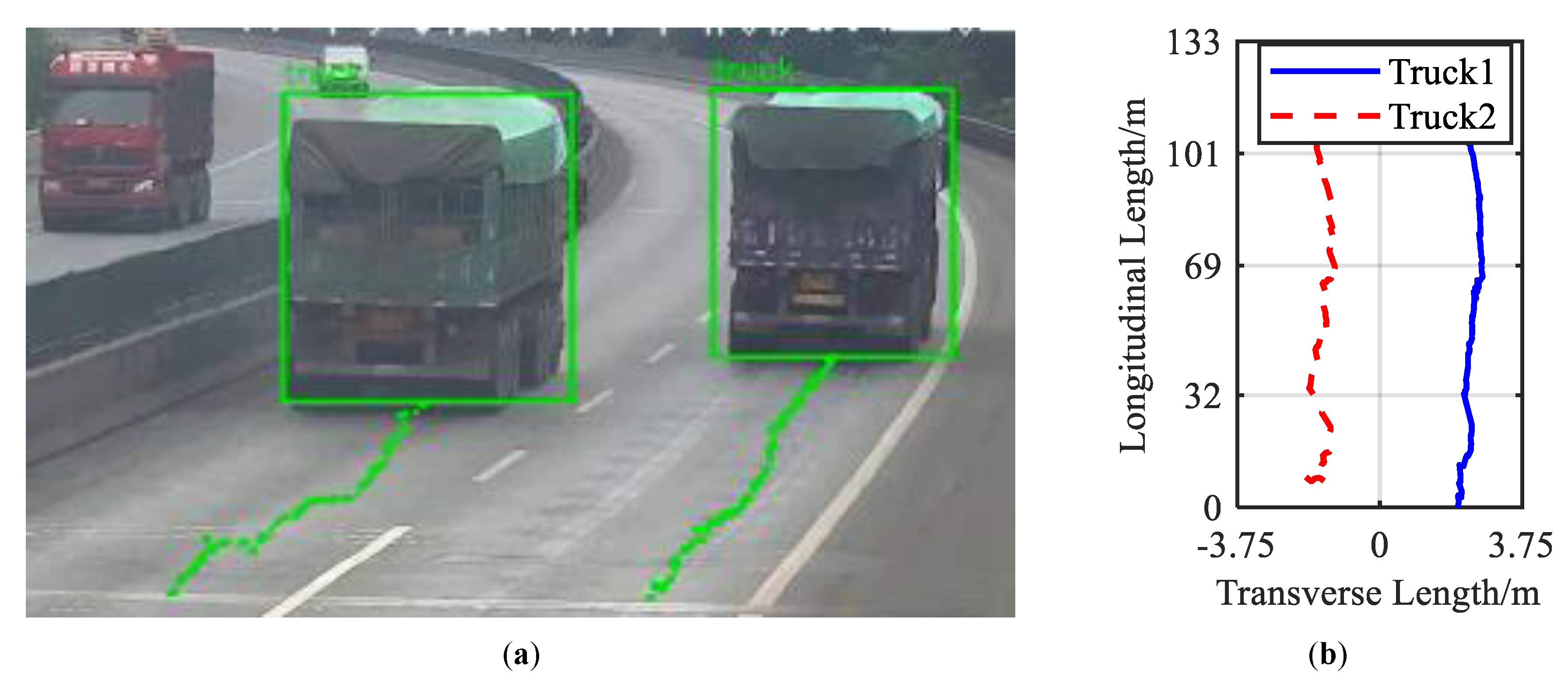
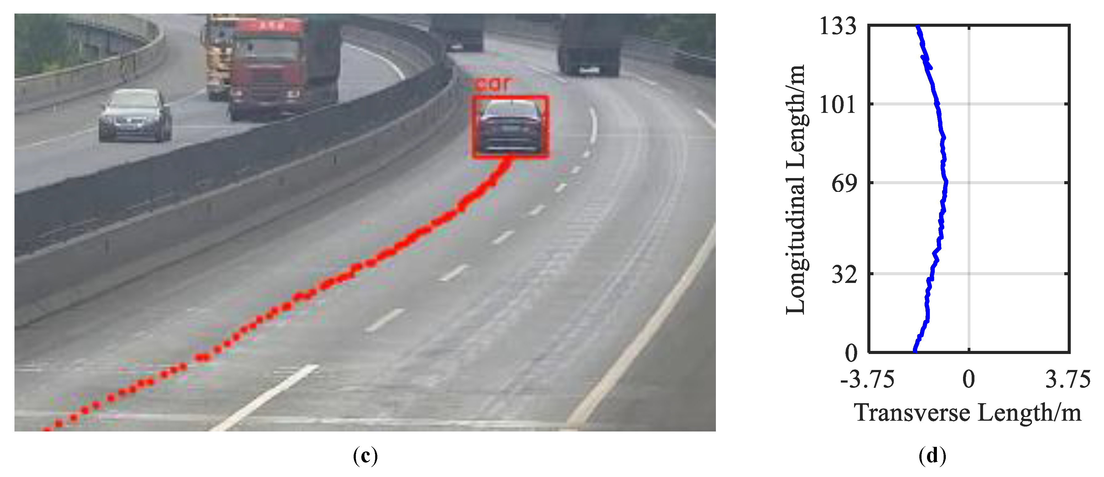
5.2. Vehicle Trajectory Recognition

The recognition of vehicle trajectory plays a vital role in solving the multiple-vehicle problem. The influence values of multiple vehicles, which are essential for forming the inverse influence line equation in order to estimate the gross vehicle weight, cannot be obtained without knowing their real-time positions. As aforementioned, the computer vision technique makes it feasible to locate vehicles in every video frame so that the vehicle trajectory can be recognized, as shown in Figure 8, depicting vehicle trajectories tracked by the aforementioned method.

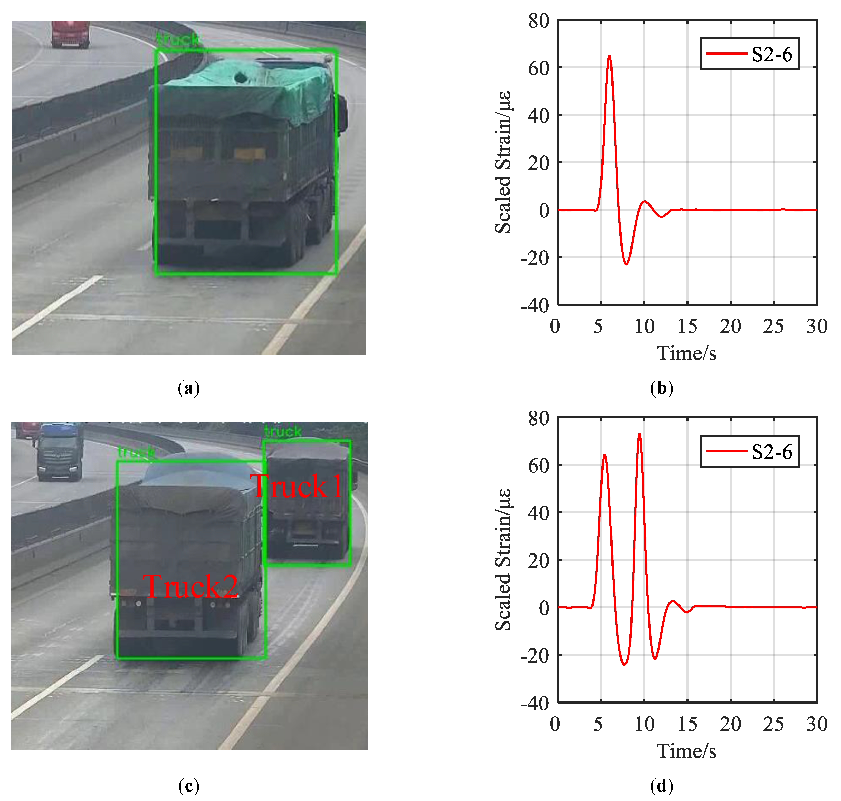
5.3. Identification Results for Complex Scenarios

As for simple traffic scenarios such as only one vehicle passing the bridge, the recognition of vehicle type, velocity and axle numbers has already been performed with certain accuracy [30]. This paper would focus on a more challenging problem: elaborating the GVW recognition method on the multiple-vehicle problem that remains to be solved. In general, there are three elementary scenarios of vehicle distribution: i) single vehicle as seen in Figure 9a, ii) one-by-one vehicles on the same lane as seen in Figure 9b and iii) side-by-side vehicles on different lanes as shown in Figure 9c.

5.3.1. Scenario: One-By-One Vehicles

The highway bridge chosen in the field tests has the span length of 32 + 37 + 32 + 32 = 133 m. Oftentimes, one-by-one vehicles drive simultaneously on the bridge. However, a sizeable safety margin, no less than 50 m, between the front and rear vehicles is demanded when driving on highways in China. That explains why two peaks can be observed clearly in the bridge strain signal caused by moving vehicles, as Figure 9d illustrates. Moreover, the demand provides the advantage that the front vehicle would add little to the bridge strain caused by the rear one. A 50 m margin means when the rear vehicle enters the first span of the bridge, the front vehicle has already reached the third or fourth span. According to the influence line in Figure 7, the influence value of the third and fourth span is far smaller than the first span. In conclusion, the one-by-one vehicles scenario in this research can be simplified as the single vehicle scenario and the GVW of each vehicle can be calculated using the aforementioned Equation (12) with the corresponding peak of the strain signal.

To verify the accuracy of the simplification above, the GVW of the two trucks in Figure 9c are calculated and the process is listed in

Table 1. GVW recognition process in a one-by-one vehicles scenario.

Vehicle Name	Truck1	Truck2
①Maximum strain	64.21	73.00
②Maximum influence value of sensor S2-6	1.396	1.396
③GVW = ①/②	46.00 t	52.29 t
④GVW measured by pavement-based WIM	50.37 t	50.69 t
Error = (③−④)/④	−8.67%	3.16%

. Errors of the recognition results are acceptable, as listed in Table 1.

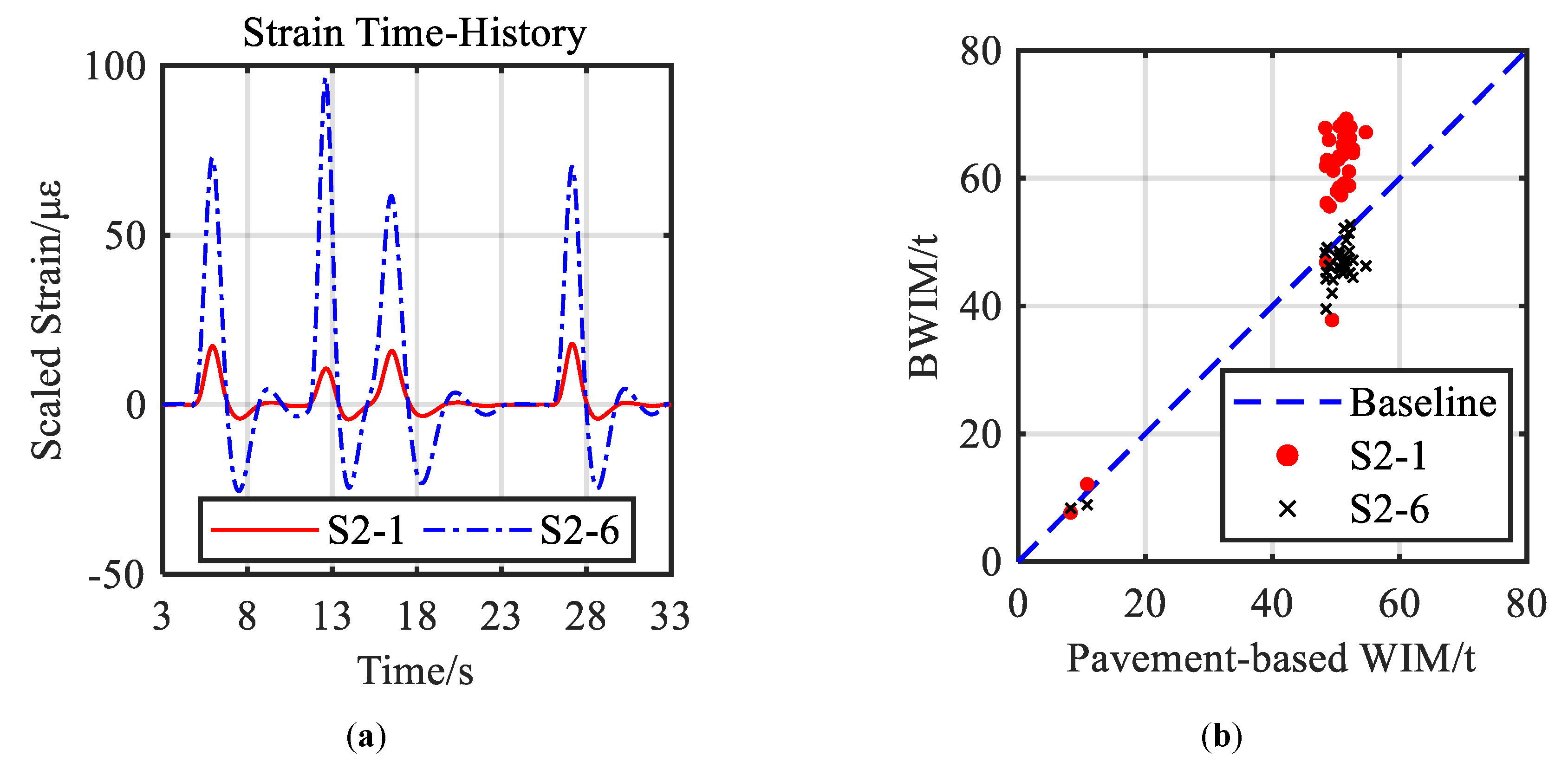
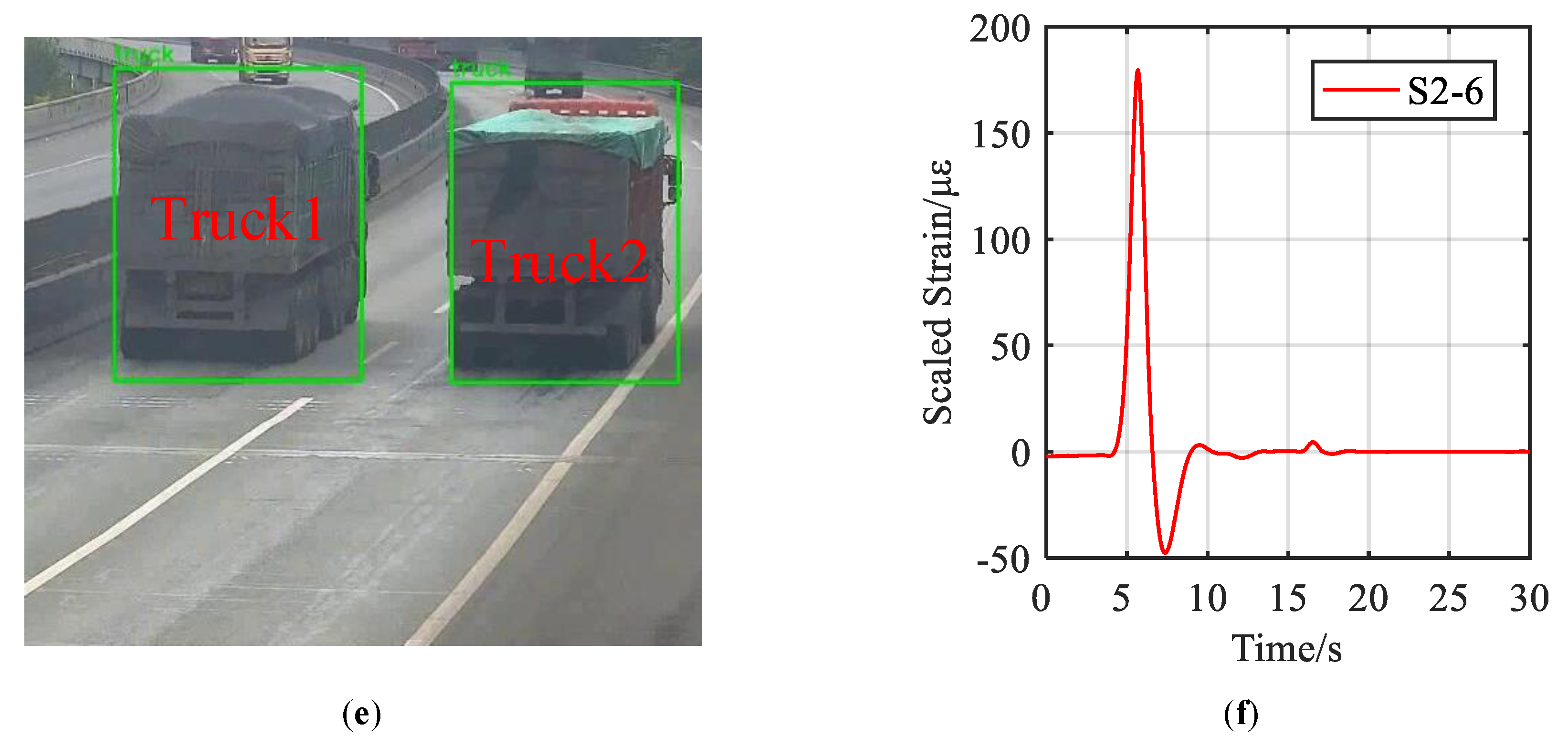
5.3.2. Scenario: Side-By-Side Vehicles

Challenge arises when two vehicles are driving side by side. In this scenario, one single strain signal peak in Figure 9f comprises two indistinguishable vehicles, making the above GVW recognition methods ineffective. According to Yu et al. [10], the identification of multiple-vehicle presence is still one of the main challenges faced by BWIM technique.

In order to solve this problem, it is necessary to integrate strain data of multiple strain sensors so that the previous Equation (14) can be used. Theoretically, two sensors are enough to determine two unknown GVW according to the linear algebra. However, the GVW results might vary considerably due to the inevitable measuring errors existing in field tests. One practical method to mitigate the variation is augmenting additional strain sensors to make the constraints exceed the unknowns and use the least squares to solve the overdetermined problem, as the text Section 3.3 has stated.

Taking the two trucks in Figure 9e as an example, a comprehensive explanation is given as follows. At the moment shown in the figure, the distances between the two trucks and the start line of the bridge are 16.1 m and 17.8 m, respectively, given by the visual sensing technique. According to the distances and the calibrated influence line, corresponding influence values of the trucks can be found as listed in the

Table 2. GVW recognition information in side-by-side vehicles scenario.

Sensor Name	Strain (με)	Influence Value (με/ton)
		Truck1	Truck2
S2-2	94.3	1.01	0.75
S2-3	158.5	1.62	1.22
S2-5	112.8	0.71	1.33
S2-6	179.6	1.20	2.14

. The strain values at that moment are listed as well.

Based on the information of sensor ‘S2-2’ and ‘S2-3’ in Table 2, the formula for calculating the GVW of the side-by-side vehicles is written as follows:

$$\{\begin{array}{l}1.01W_1+0.75W_2=94.3\\ 1.62W_1+1.22W_2=158.5\end{array},$$

(18)

where W₁ and W₂ are the GVW of truck1 and truck2 in Figure 9e. The recognition results are W₁ = −222.62 t and W₂ = 425.52 t, which are clearly wrong.

Then, the recognition equation is rewritten using information of four sensors as follows:

$$\{\begin{array}{l}1.01W_1+0.75W_2=94.3\\ 1.62W_1+1.22W_2=158.5\\ 0.71W_1+1.33W_2=112.8\\ 1.20W_1+2.14W_2=179.6\end{array},$$

(19)

The least square method is used to solve the overdetermined equation and the results are W₁ = −57.06 t and W₂ = −52.63 t. The GVWs measured by the pavement-based WIM system are 51.12 t and 49.12 t. The error between the BWIM and the pavement-based WIM is acceptable, which means the problem of when two vehicles drive side-by-side is successfully solved.

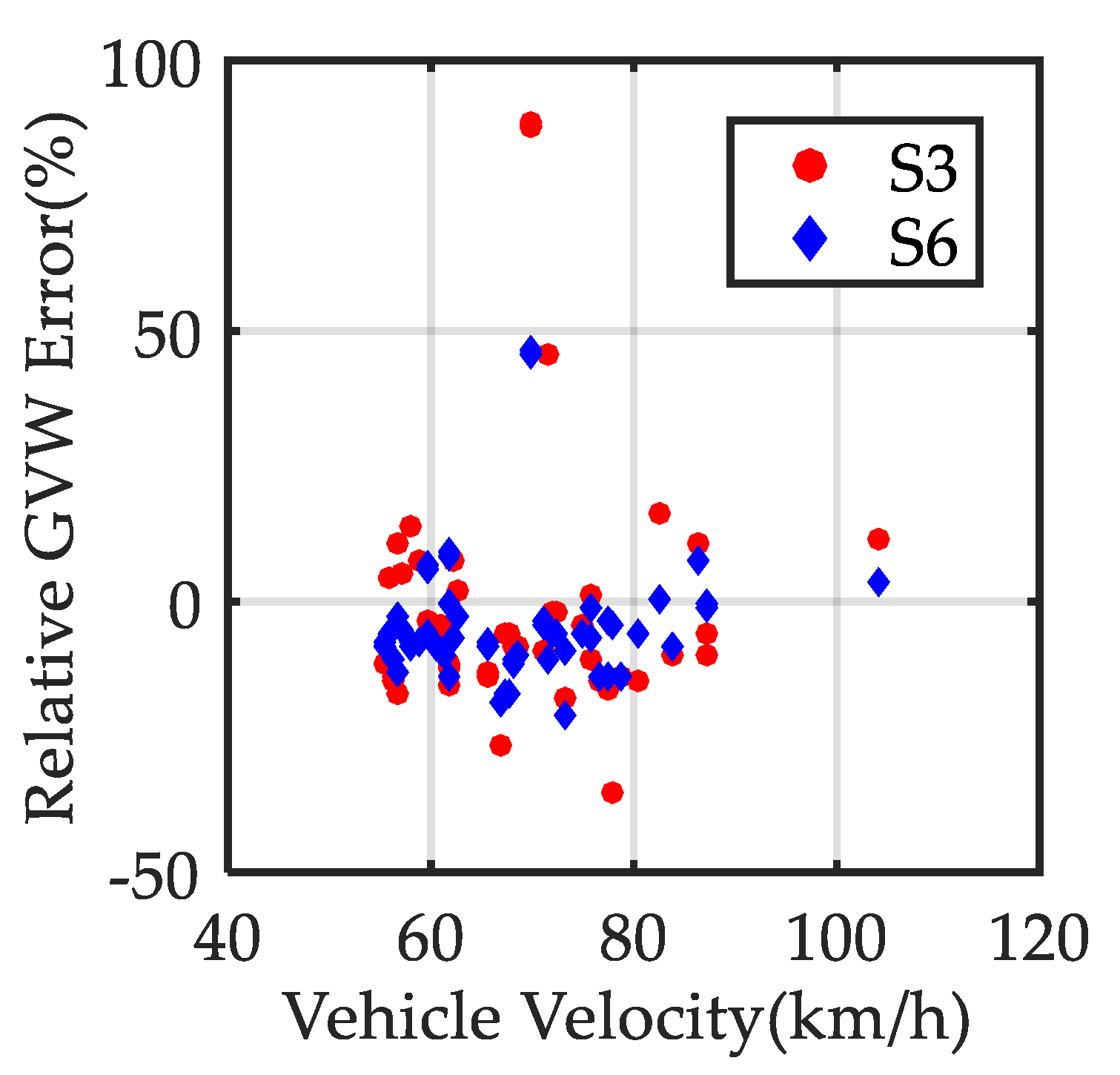
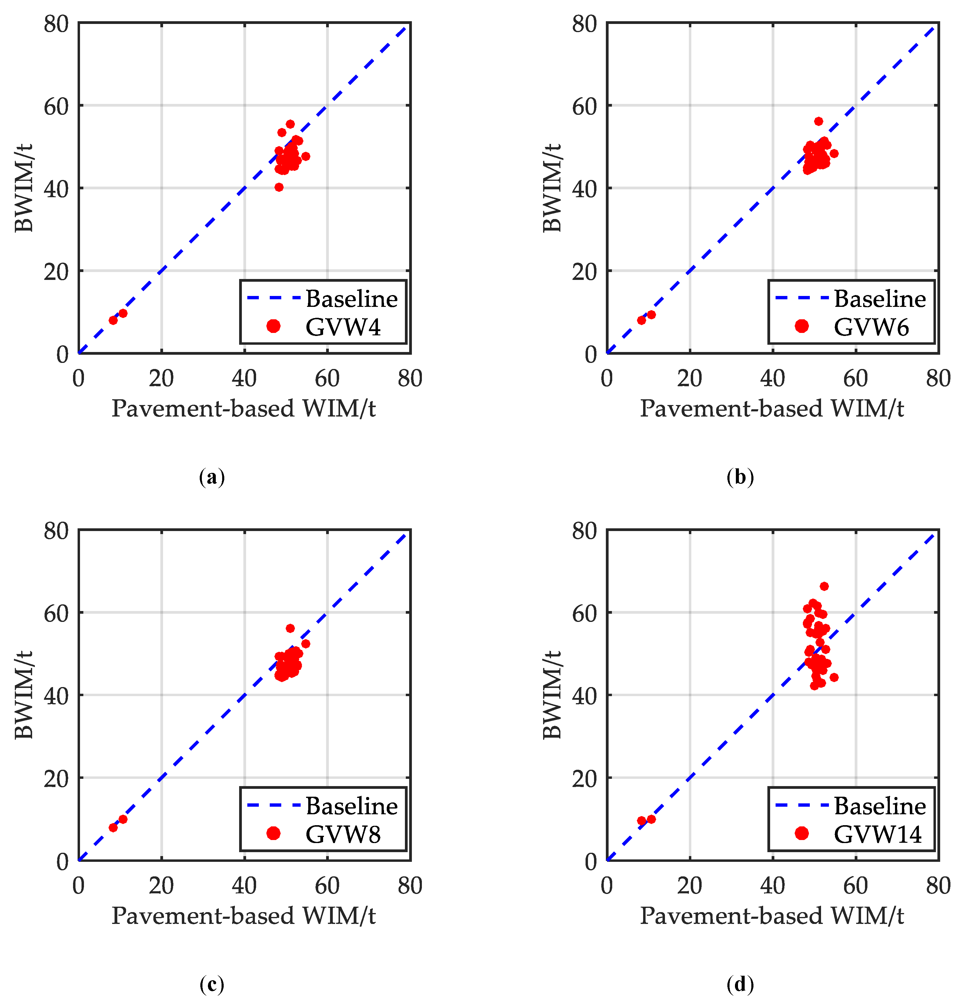
5.3.3. Statistical Analysis for Identification Results

For a more persuasive verification, a segment of a 5 min strain signal and a video when all the three scenarios of vehicle distribution exist are statistically analyzed for illustration. Cars are ignored, because cars (less than 3 tons) are much lighter than trucks (20~60 tons); thus, neglecting cars will not bring significant weighing error. Additionally, heavy trucks are more dangerous to bridge structures compared to ordinary cars. In fact, most BWIM research mainly focus on trucks as only trucks are closely noticed by the traffic and bridge management department. The GVWs of a total of 38 trucks were calculated. Different numbers of strain sensors were used to investigate the effects of taking the least square method to solve the inverse influence line theory equations. The recognition results of the GVW are presented in

Table 3. Recognition results of the GVW.

Truck Number	Scenario	GVW-WIM(t)	GVW-BWIM-4 Sensors(t)	GVW-BWIM-6 Sensors(t)	GVW-BWIM-8 Sensors(t)	GVW-BWIM-14 Sensors(t)
1	single	53.12	51.48	50.49	49.84	47.72
2	single	50.93	48.29	49.02	47.95	47.13
3	side-by-side	51.12	55.56	56.22	56.15	56.64
4	side-by-side	49.12	53.33	50.27	49.37	50.91
5	one-by-one	50.37	48.59	49.04	48.85	49.15
6	one-by-one	50.69	47.31	47.39	48.09	61.60
7	single	51.29	50.13	50.44	50.39	56.04
8	single	51.09	47.92	47.83	48.14	54.91
9	single	49.54	44.27	45.01	44.67	62.34
10	single	51.61	49.83	50.06	49.93	48.66
11	single	8.23	8.03	8.01	8.02	9.70
12	single	48.42	44.66	44.80	44.74	56.98
13	single	48.58	46.96	47.49	47.18	48.11
14	single	50.49	45.85	46.00	45.95	54.73
15	single	51.33	47.77	47.74	47.73	43.01
16	single	51.65	47.99	48.47	48.34	42.72
17	side-by-side	52.16	47.01	47.33	47.12	55.57
18	side-by-side	48.43	40.17	44.19	45.06	57.61
19	single	52.25	51.57	51.46	50.58	66.20
20	one-by-one	50.55	49.17	49.91	49.94	43.72
21	one-by-one	50.78	47.10	46.09	47.06	55.06
22	single	48.51	46.66	46.12	46.49	50.20
23	single	54.68	47.61	48.24	52.44	44.07
24	single	52.67	46.68	45.87	47.39	51.01
25	single	52.05	45.39	45.50	45.49	45.86
26	side-by-side	48.88	46.89	46.95	46.87	58.51
27	side-by-side	49.37	46.87	45.91	46.96	47.18
28	one-by-one	52.66	46.67	46.90	46.91	56.05
29	one-by-one	50.35	45.38	45.68	45.62	44.45
30	single	51.06	46.62	46.71	46.60	56.21
31	single	10.83	9.58	9.46	9.94	10.09
32	single	48.97	44.12	44.48	44.29	55.19
33	single	52.01	48.21	48.09	48.73	59.53
34	single	51.06	46.76	46.96	46.82	59.95
35	single	51.28	45.24	45.62	45.37	52.58
36	single	50.14	45.13	45.76	45.30	42.21
37	single	50.46	45.43	45.81	45.66	46.14
38	single	48.30	48.88	49.49	49.48	60.69

, in which the ‘GVW-WIM’ is the GVW measured by the WIM system, ‘GVW-BWIM-4 Sensors’ are the GVW identified with strain sensors ‘S2-2’, ‘S2-3’, ‘S2-5’, and ‘S2-6’. The ‘GVW-BWIM-6 Sensors’ are the GVW identified with strain sensors ‘S2-2’, ‘S2-3’, ‘S2-5’, ‘S2-6’, ‘S1-2’, and ‘S1-4’. The ‘GVW-BWIM-8 Sensors’ are the GVW identified with strain sensors ‘S2-2’, ‘S2-3’, ‘S2-5’, ‘S2-6’, ‘S1-2’, ‘S1-4’, ‘S3-2’, and ‘S3-4’. The ‘GVW-BWIM-14 Sensors’ are the GVW identified with all the strain sensors mounted on the bridge.

Table 3 gives detailed identification results of a total of 38 vehicles in various traffic scenarios. The GVW of each vehicle was identified using partial or all of the available 14 strain sensors in order to compare and quantitatively optimize the number of sensors and the location of sensors. Comprehensively, Table 3 concludes as follows:

• The recognition results of the GVW are of acceptable accuracy when using data from less than eight strain sensors;
• Errors in one-by-one and side-by-side vehicle scenarios are slightly larger in contrast to the single vehicle scenario. The difference is reasonable because the position of vehicles is essential to obtain their influence value when recognizing the GVW in complicated traffic scenarios, and the positioning error is inevitable in the process of coordinate transformation.
• An interesting phenomenon is the obvious larger error when using the data from all 14 strain sensors. Detailed reason would be particularly discussed later.

Intuitive plots of the GVW results for different numbers of strain sensors are shown in Figure 10, in which each point corresponds to a vehicle. In these figures, the further away the point is from the baseline, the larger the error is.

Statistics of the relative errors compared with the results recognized by the pavement-based WIM system are also listed in

Table 4. Statistics of the relative errors compared with pavement-based WIM.

Number of Sensors	Mean of Errors (%)	Standard Deviation of Errors (%)	Maximum Error (%)
4	−7.66	4.07	+1.20/−17.06
6	−7.20	3.80	+2.46/−12.91
8	−6.69	3.46	+2.44/−12.60
14	3.69	13.41	+26.70/−19.40

. The statistics show that due to the introduction of more redundant information, the more strain sensors of the sensor network are used, the smaller the error is.

Finally, it is necessary to highlight the reason behind the large error caused by the usage of all 14 strain sensors. Compared with the scenario using eight sensors, the extra six sensors are mounted close to the neutral axis of the bridge cross-section. According to the Euler-Bernoulli beam theory [39], the closer a strain sensor is to the neutral axis, the smaller its strain value, making the relative error lager in contrast. Figure 11 compares the time-history curves and the GVW recognition results of two strain sensors, S2-1 and S2-6, whose distances to the neutral axis are 100 mm and 800 mm, respectively. Errors of the sensor ‘S2-1’ are obviously more significant than those of the sensor ‘S2-6’. To avoid this problem, strain sensors for BWIM purposes should be installed far from the section neutral axis for higher accuracy.

Previous studies also point out that road roughness and vehicle velocity will affect the GVW recognition accuracy because of the vehicle-bridge coupling vibration. The faster the vehicle drives, the larger the GVW recognition errors are [40]. However, according to the obtained results, this issue is not significant in this research. This is because, on one hand, vehicle-bridge coupling vibration effects are almost eliminated by the preceding LOWESS algorithm; on the other hand, road surface of highway is quite smooth, thus, severe vehicle-bridge coupling vibration will not be excited though vehicles driving at high velocity. Figure 12 proves that vehicle velocity does not induce GVW recognition errors in sensors S2-3 and S2-6, as no obvious pattern can be found in the scatter plot.

6. Conclusions

With special focus on complicated traffic scenarios, this paper presents a traffic load identification methodology using multiple strain sensors and single camera for short and medium span bridges. Systematic field tests were performed on a concrete box-girder bridge to investigate the reliability and accuracy of the proposed method in practice. Based on the results, the following conclusions are drawn:

• Deep learning based computer vision technique is a practical tool to extract the key parameters from traffic video in real time manner, such as position, size, axle number and type of passing vehicles over bridge. Moreover, traffic mode of multi-vehicle problem is equally important to be identified as one-by-one, side-by-side or mixed mode.
• By utilizing the redundant strain measurements, the proposed least square based identification method is capable of: i) distinguishing complicated traffic mode such as side-by-side vehicles, which is theoretically unidentifiable with single measurement and ii) solving the overdetermined inverse influence equations effectively, and hence, reducing the GVW recognition errors.
• Under the condition that vehicle parameters (especially positions) are identified and available, the proposed framework successfully recognizes the vehicle weight in spite of the presence of one-by-one and side-by-side vehicles, with an average weighing error less than 8%. Thus, the elementary scenarios of the multiple-vehicle problem for BWIM research are solved with an overall improvement with respect to cost and accuracy.
• The usage of strain sensors installed at locations with larger response results in smaller recognition error of vehicle weight. It is suggested that strain sensors for BWIM purposes should be installed far from the neutral axis of cross-sections for the sake of higher accuracy.

References

1. Hu, X.; Wang, B.; Ji, H. A wireless sensor network-based structural health monitoring system for highway bridges. Comput.-Aided Civ. Infrastruct. Eng. 2013, 28, 193–209. [Google Scholar] [CrossRef]
2. Farrar, C.R.; Park, G.; Allen, D.W.; Todd, M.D. Sensor network paradigms for structural health monitoring. Struct. Control Health Monit. 2006, 13, 210–225. [Google Scholar] [CrossRef]
3. Cheng, L.; Pakzad, S.N. Agility of Wireless Sensor Networks for Earthquake Monitoring of Bridges. In Proceedings of the Sixth International Conference on Networked Sensing Systems (INSS), Pittsburgh, PA, USA, 17–19 June 2009; pp. 1–4. [Google Scholar]
4. Jo, H.; Sim, S.H.; Mechitov, K.A.; Kim, R.; Li, J.; Moinzadeh, P.; Spencer, B.F., Jr.; Park, J.W.; Cho, S.; Jung, H.J.; et al. Hybrid wireless smart sensor network for full-scale structural health monitoring of a cable-stayed bridgeSensors and Smart Structures Technologies for Civil, Mechanical, and Aerospace Systems 2011. Int. Soc. Opt. Photonics 2011, 7981, 798105. [Google Scholar]
5. Feng, D.M.; Feng, M.Q. Identification of structural stiffness and excitation forces in time domain using noncontact vision-based displacement measurement. J. Sound Vib. 2017, 406, 15–28. [Google Scholar] [CrossRef]
6. Feng, D.M.; Feng, M.Q. Experimental validation of cost-effective vision-based structural health monitoring. Mech. Syst. Signal Process. 2017, 88, 199–211. [Google Scholar] [CrossRef]
7. Fraser, M.; Elgamal, A.; He, X.; Conte, J.P. Sensor network for structural health monitoring of a highway bridge. J. Comput. Civ. Eng. 2009, 24, 11–24. [Google Scholar] [CrossRef]
8. Rutherford, G.; McNeill, D.K. Statistical vehicle classification methods derived from girder strains in bridges. Can. J. Civ. Eng. 2010, 38, 200–209. [Google Scholar] [CrossRef]
9. Gonzalez, I.; Karoumi, R. Traffic monitoring using a structural health monitoring system. Proc. ICE-Bridge Eng. 2014, 168, 13–23. [Google Scholar]
10. Yu, Y.; Cai, C.S.; Deng, L. State-of-the-art review on bridge weigh-in-motion technology. Adv. Struct. Eng. 2016, 19, 1514–1530. [Google Scholar] [CrossRef]
11. Moses, F. Weigh-in-motion system using instrumented bridges. J. Transp. Eng. 1979, 105, 233–249. [Google Scholar]
12. Lydon, M.; Taylor, S.E.; Robinson, D.; Mufti, A.; Brien, E.J. Recent developments in bridge weigh in motion (B-WIM). J. Civ. Struct. Health Monit. 2016, 6, 69–81. [Google Scholar] [CrossRef]
13. Zhu, X.Q.; Law, S.S. Recent developments in inverse problems of vehicle–bridge interaction dynamics. J. Civ. Struct. Health Monit. 2016, 6, 107–128. [Google Scholar] [CrossRef]
14. Schmidt, F.; Jacob, B.; Servant, C.; Marchadour, Y. Experimentation of a Bridge WIM System in France and Applications for Bridge Monitoring and Overload Detection. In Proceedings of the 6th International Conference on Weigh-In-Motion (ICWIM 6), Dallas, TX, USA, 4–7 June 2012. [Google Scholar]
15. Snyder, R.; Moses, F. Application of in-motion weighing using instrumented bridges. Transp. Res. Rec. 1985, 1048, 83–88. [Google Scholar]
16. Yu, Y.; Cai, C.S.; Deng, L. Nothing-on-road bridge weigh-in-motion considering the transverse position of the vehicle. Struct. Infrastruct. Eng. 2018, 14, 1108–1122. [Google Scholar] [CrossRef]
17. Deng, L.; He, W.; Yu, Y.; Cai, C.S. Equivalent shear force method for detecting the speed and axles of moving vehicles on bridges. J. Bridge Eng. 2018, 23, 04018057. [Google Scholar] [CrossRef]
18. He, W.; Ling, T.; OBrien, E.J.; Deng, L. Virtual Axle Method for Bridge Weigh-in-Motion Systems Requiring No Axle Detector. J. Bridge Eng. 2019, 24, 04019086. [Google Scholar] [CrossRef]
19. Basharat, A.; Catbas, N.; Shah, M. A Framework for Intelligent Sensor Network with Video Camera for Structural Health Monitoring of Bridges. In Proceedings of the Third IEEE International Conference on Pervasive Computing and Communications Workshops, Kauai Island, HI, USA, 8–12 March 2005; pp. 385–389. [Google Scholar]
20. Chen, Z.; Li, H.; Bao, Y.; Li, N.; Jin, Y. Identification of spatio-temporal distribution of vehicle loads on long-span bridges using computer vision technology. Struct. Control Health Monit. 2016, 23, 517–534. [Google Scholar] [CrossRef]
21. Hou, R.; Jeong, S.; Wang, Y.; Law, K.H.; Lynch, J.P. Camera-based Triggering of Bridge Structural Health Monitoring Systems using a Cyber-physical System Framework. In Proceedings of the 11th International Workshop on Structural Health Monitoring, Stanford, CA, USA, 12–14 September 2017. [Google Scholar]
22. Feng, D.M.; Feng, M.Q. Computer vision for SHM of civil infrastructure: From dynamic response measurement to damage detection—A review. Eng. Struct. 2018, 156, 105–117. [Google Scholar] [CrossRef]
23. Dan, D.; Ge, L.; Yan, X. Identification of moving loads based on the information fusion of weigh-in-motion system and multiple camera machine vision. Measurement 2019, 144, 155–166. [Google Scholar] [CrossRef]
24. Rawat, W.; Wang, Z. Deep convolutional neural networks for image classification: A comprehensive review. Neural Comput. 2017, 29, 2352–2449. [Google Scholar] [CrossRef]
25. Kaushal, M.; Khehra, B.S.; Sharma, A. Soft Computing based object detection and tracking approaches: State-of-the-Art survey. Appl. Soft Comput. 2018, 70, 423–464. [Google Scholar] [CrossRef]
26. Schmidhuber, J. Deep learning in neural networks: An overview. Neural Netw. 2015, 61, 85–117. [Google Scholar] [CrossRef] [PubMed]
27. Girshick, R.; Donahue, J.; Darrell, T.; Malik, J. Rich Feature Hierarchies for Accurate Object Detection and Semantic Segmentation. In Proceedings of the IEEE Conference on Computer Vision and Pattern Recognition, Columbus, OH, USA, 24–27 January 2014; pp. 580–587. [Google Scholar]
28. He, K.; Gkioxari, G.; Dollár, P.; Girshick, R. Mask R-CNN. In Proceedings of the IEEE International Conference on Computer Vision, Venice, Italy, 22–29 October 2017; pp. 2961–2969. [Google Scholar]
29. Xu, G.; Zhang, Z. Epipolar Geometry in Stereo, Motion and Object Recognition: A Unified Approach, 1st ed.; Kluwer Academic Publisher: Dordrecht, The Netherlands, 1996. [Google Scholar]
30. Jian, X.; Xia, Y.; Lozano-Galant, J.A.; Sun, L. Traffic Sensing Methodology Combining Influence Line Theory and Computer Vision Techniques for Girder Bridges. J. Sens. 2019, 2019, 3409525. [Google Scholar] [CrossRef]
31. Cleveland, W.S.; Devlin, S.J. Locally weighted regression: An approach to regression analysis by local fitting. J. Am. Stat. Assoc. 1988, 83, 596–610. [Google Scholar] [CrossRef]
32. Ma, H.Y.; Shi, X.F.; Zhang, Y. Long-Term Behavior of Precast Concrete Deck Using Longitudinal Prestressed Tendons in Composite I-Girder Bridge. Appl. Sci. 2018, 8, 2598. [Google Scholar] [CrossRef]
33. Znidaric, A.; Baumgartner, W. Bridge Weigh-in-Motion Systems-an Overview. In Proceedings of the Second European Conference on Weigh-in-Motion of Road Vehicles, Lisbon, Portugal, 14–16 September 1998. [Google Scholar]
34. McNulty, P.; O’Brien, E.J. Testing of bridge weigh-in-motion system in a sub-Arctic climate. J. Test. Eval. 2003, 31, 497–506. [Google Scholar]
35. O’Brien, E.J.; Quilligan, M.; Karoumi, R. Calculating an influence line from direct measurements. Bridge Eng. Proc. Inst. Civ. Eng. 2006, 159, 31–34. [Google Scholar] [CrossRef]
36. Zhao, H.; Uddin, N.; Shao, X.; Zhu, P.; Tan, C. Field-calibrated influence lines for improved axle weight identification with a bridge weigh-in-motion system. Struct. Infrastruct. Eng. 2015, 11, 721–743. [Google Scholar] [CrossRef]
37. Young, D.H.; Timoshenko, S.P. Theory of Structures; McGraw-Hill: New York, NY, USA, 1965. [Google Scholar]
38. Lawson, C.L.; Hanson, R.J. Solving Least Squares Problems, 1st ed.; Prentice-Hall Inc.: Englewood Cliffs, NJ, USA, 1974. [Google Scholar]
39. Timoshenko, S.P.; Gere, J.M. Mechanics of Materials; Van Nordstrand Reinhold Company: New York, NY, USA, 1972. [Google Scholar]
40. Leming, S.K.; Stalford, H.L. Bridge Weigh-in-Motion System Development Using Superposition of Dynamic Truck/Static Bridge Interaction. In Proceedings of the IEEE 2003 American Control Conference, Denver, CO, USA, 4–6 June 2003; Volume 1, pp. 815–820. [Google Scholar]
Figure 1. Vehicle recognition results. (a) Before entering the bridge deck; (b) after entering the bridge deck.
Remotesensing 11 02651 g001
Figure 2. Coordinate systems. (a) Diagram of coordinate systems; (b) spatial camera imaging model; (c) planar camera imaging model.
Remotesensing 11 02651 g002
Figure 3. Procedure of the vehicle induced static strain extraction.
Remotesensing 11 02651 g003
Figure 4. Diagram of the influence line calibration method.
Remotesensing 11 02651 g004
Figure 5. Data integration framework.
Remotesensing 11 02651 g005
Figure 6. Instrumentation of bridge system for field tests. (a) diagram; (b) longitudinal elevation. WIM: weigh-in-motion.
Remotesensing 11 02651 g006
Figure 7. Calibrated influence lines on the traffic lane. (a) Traffic line 1; (b) Traffic line 2.
Remotesensing 11 02651 g007aRemotesensing 11 02651 g007b
Figure 8. Vehicle trajectory recognition. (a) Truck trajectories in image, (b) truck trajectories on bridge deck, (c) car trajectory in image and (d) car trajectory on bridge deck.
Remotesensing 11 02651 g008aRemotesensing 11 02651 g008b
Figure 9. Scenarios of vehicle distribution on bridge. (a) Single vehicle, (b) strain signal of single vehicle, (c) one-by-one vehicles, (d) strain signal of one-by-one vehicles, (e) side-by-side vehicles and (f) strain signal of side-by-side vehicles.
Remotesensing 11 02651 g009aRemotesensing 11 02651 g009b
Figure 10. GVW recognition results for different numbers of strain sensors. (a) GVW results using four sensors (b) GVW results using six sensors (c) GVW results using eight sensors (d) GVW results using 14 sensors.
Remotesensing 11 02651 g010
Figure 11. Comparison between two sensors. (a) Bridge strain time-history curves; (b) GVW recognition results.
Remotesensing 11 02651 g011
Figure 12. Correlation of velocity and relative GVW errors.
Remotesensing 11 02651 g012