Watson on the Farm: Using Cloud-Based Artificial Intelligence to Identify Early Indicators of Water Stress

 ,
,  ,
,  and
and 
Abstract
:
1. Introduction
2. Materials and Methods
2.1. Image Acquisition
2.2. Image Pre-Processing
2.3. Model Training and Testing
2.4. Statistical Analysis
3. Results
4. Discussions
5. Conclusions
Author Contributions
Funding
Acknowledgments
Conflicts of Interest
References
- Maja, J.M.; Robbins, J. Controlling irrigation in a container nursery using IoT. AIMS Agric. Food 2018, 3, 205–215. [Google Scholar] [CrossRef]
- Cohen, Y.; Alchanatis, V.; Meron, M.; Saranga, S.; Tsipris, J. Estimation of leaf water potential by thermal imagery and spatial analysis. J. Exp. Bot. 2005, 56, 1843–1852. [Google Scholar] [CrossRef] [PubMed]
- Gago, J.; Douthe, C.; Coopman, R.E.; Gallego, P.P.; Ribas-Carbo, M.; Flexas, J.; Escalona, J.; Medrano, H. UAVs challenge to assess water stress for sustainable agriculture. Agric. Water Manag. 2015, 153, 9–19. [Google Scholar] [CrossRef]
- Jacobson, B.K.; Jones, P.H.; Jones, J.W.; Paramore, J.A. Real-time greenhouse monitoring and control with an expert system. Comput. Electron. Agric 1989, 3, 273–285. [Google Scholar] [CrossRef]
- Kim, Y.; Evans, A.R.G. Software design for wireless sensor-based site-specific irrigation. Comput. Electron. Agric. 2009, 66, 159–165. [Google Scholar] [CrossRef]
- Stone, K.C.; Smajstrla, A.G.; Zazueta, F.S. Microcomputer-based data acquisition system for continuous soilwater potential measurements. Soil Crop Sci. Soc. Fla. Proc. 1985, 44, 49–53. [Google Scholar]
- Coates, R.W.; Delwiche, J.M.; Brown, P.H. Design of a system for individual microsprinkler control. Trans. ASABE 2006, 49, 1963–1970. [Google Scholar] [CrossRef]
- USDA; National Agricultural Service. 2017 Census of Agriculture, United States Summary and State Data; Geographic Area Series, Part 51. Publ AC-17-A-51; USDA: Washington, DC, USA; National Agricultural Service: Washington, DC, USA, 2019; Volume1, p. 820.
- Vilsack, T.; Reilly, A.J.T. 2012 Census of Agriculture. Census of Horticultural Specialties (2014); Special Studies. Part 3. AC-12-SS-3; 2015; Volume 3, p. 422. Available online: https://www.nass.usda.gov/Publications/AgCensus/2012/Online_Resources/Farm_and_Ranch_Irrigation_Survey/fris13.pdf (accessed on 8 November 2019).
- Vilsack, T.; Reilly, A.J.T. 2012 Census of Agriculture. Farm and Ranch Irrigation Survey (2013); Special Studies. Part 1. AC-12-SS-1; USDA NASS; Volume 3, pp. 84–195. Available online: https://www.nass.usda.gov/Publications/AgCensus/2012/Online_Resources/Farm_and_Ranch_Irrigation_Survey/fris13.pdf (accessed on 8 November 2019).
- USDA. USDA Agricultural Resource Management Survey (ARMS) 2016. Available online: https://www.ers.usda.gov/topics/farm-economy/farm-labor/ (accessed on 16 September 2019).
- Posadas, B.C.; Knight, P.R.; Coker, C.H.; Coker, R.Y.; Langlois, S.A. Hiring Preferences of Nurseries and Greenhouses in Southern United States. Hort Technol. 2014, 24, 101–117. [Google Scholar]
- Robbins, J.A. Small unmanned aircraft systems (sUAS): An emerging technology for horticulture. Hortic. Rev. 2018, 45, 33–71. [Google Scholar]
- De Castro, A.I.; Ehsani, R.; Ploetz, R.; Crane, J.H.; Abdulridha, J. Optimum spectral and geometric parameters for early detection of laurel wilt disease in avocado. Remote Sens. Environ. 2015, 171, 33–44. [Google Scholar] [CrossRef]
- De Castro, A.I.; Torres-Sánchez, J.; Peña, J.M.; Jiménez-Brenes, F.M.; Csillik, O.; López-Granados, F. An Automatic Random Forest-OBIA Algorithm for Early Weed Mapping between and within Crop Rows Using UAV Imagery. Remote Sens. 2018, 10, 285. [Google Scholar] [CrossRef]
- Maja, J.M.; Campbell, T.; Camargo-Neto, J.; Astillo, P. Predicting cotton yield of small field plots in a cotton breeding program using UAV imagery data. In Proceedings of the Autonomous Air and Ground Sensing Systems for Agricultural Optimization and Phenotyping, Baltimore, MD, USA, 17 May 2016; p. 98660C. [Google Scholar] [CrossRef]
- Reay-Jones, F.; Greene, J.; Maja, J.M.; Bauer, P. Using remote sensing to improve the management of stink bugs in cotton in South Carolina. In Proceedings of the XXV International Congress of Entomology, Orlando, FL, USA, 26 September 2016. [Google Scholar]
- De Castro, A.; Maja, J.M.; Owen, J.; Robbins, J.; Peña, J.M. 2018. Experimental approach to detect water stress in ornamental plants using sUAS-imagery. In Proceedings of the Autonomous Air and Ground Sensing Systems for Agricultural Optimization and Phenotyphing, SPIE Commercial + Scientific Sensing and Imaging, Orlando, FL, USA, 21 May 2018. [Google Scholar] [CrossRef]
- Salami, E.; Barrado, C.; Pastor, E. UAV flight experiments applied to remote sensing of vegetated areas. Remote Sens. 2014, 6, 11051–11081. [Google Scholar] [CrossRef]
- Shahbazi, M.; Jérôme, T.; Ménard, P. Recent applications of unmanned aerial imagery in natural resource management. GISci. Remote Sens. J. 2014, 51, 1548–1603. [Google Scholar] [CrossRef]
- Jackson, R.D. Canopy temperature and crop water stress. In Advances in Irrigation; Hillel, D., Ed.; Academic Press: New York, NY, USA, 1982; Volume 1, pp. 43–80. [Google Scholar]
- Bellvert, J.; Zarco-Tejada, P.J.; Girona, J.; Fereres, E. Mapping crop water stress index in a ‘Pinot-noir’ vineyard: Comparing ground measurements with thermal remote sensing imagery from an unmanned aerial vehicle. Precis. Agric 2014, 15, 361. [Google Scholar] [CrossRef]
- Garcia Ruiz, F.; Sankaran, S.; Maja, J.M.; Lee, W.S.; Rasmussen, J.; Ehsani, R. Comparison of two aerial imaging platforms for identification of Huanglongbing-infected citrus trees. Comput. Electron. Agric. 2013, 91, 106–115. [Google Scholar] [CrossRef]
- Stagakis, S.; Gonzalez-Dugo, V.; Cid, P.; Guillen-Climent, M.L.; Zarco-Tejada, P.J. Monitoring water stress and fruit quality in an orange orchard under regulated deficit irrigation using narrow-band structural and physiological remote sensing indices. ISPRS J. Photogramm. Remote Sens. 2012, 71, 47–61. [Google Scholar] [CrossRef]
- Zovkoa, M.; Žibrat, U.; Knapič, M.; Kovačić, M.B.; Romić, D. Hyperspectral remote sensing of grapevine drought stress. Precis. Agric 2019, 20, 335–347. [Google Scholar] [CrossRef]
- Fulcher, A.; LeBude, A.V.; Owen, J.S., Jr.; White, S.A.; Beeson, R.C. The Next Ten Years: Strategic Vision of Water Resources for Nursery Producers. HortTechnology 2016, 26, 121–132. [Google Scholar] [CrossRef]
- LeCun, Y.; Bengio, Y.; Hinton, G. Deep learning. Nature 2015, 521, 436–444. [Google Scholar] [CrossRef]
- Herent, P.; Jegoue, S.; Wainrib, G.; Clozel, T. Brain age prediction of healthy subjects on anatomic MRI with deep learning: going beyond with an “explainable AI” mindset. bioRxiv 2018, 413302. [Google Scholar] [CrossRef]
- Zhou, B.; Khosla, A.; Lapedriza, A.; Aude, O.; Torralba, A. Learning deep features for discriminative localization. arXiv 2015, arXiv:1512.04150. [Google Scholar]
- Zhang, Q.; Zhu, S. Visual interpretability for deep learning: a survey. Front. Inf. Technol. Electron. Eng. 2018, 19, 27–39. [Google Scholar] [CrossRef]
- Awad, M.; Khanna, R. Efficient Learning Machines; Springer Link Apress: Berkeley, CA, USA, 2015; pp. 167–184. ISBN 978-1-4302-5989-3. [Google Scholar]
- Ahmad, S.; Abdou, M.; Perot, E.; Yogamani, S. Deep reinforcement learning framework for autonomous driving. arXiv 2017, arXiv:1704.02532. [Google Scholar]
- Taigman, Y.; Yang, M.; Ranzato, M.; Wolf, L. DeepFace: closing the gap to human-level performance in face verification. In Proceedings of the IEEE Conference on Computer Vision and Pattern Recognition (CVPR 2014), Columbus, OH, USA, 24–27 June 2014; pp. 1701–1708. [Google Scholar]
- Knyazikhin, Y.; Schull, M.A.; Stenberg, P.; Mõttus, M.; Rautiainen, M.; Yang, Y.; Marshak, A.; Carmona, P.L.; Kaufmann, R.K.; Lewis, P. Hyperspectral remote sensing of foliar nitrogen content. Proc. Natl. Acad. Sci. USA 2013, 110, E185–E192. [Google Scholar] [CrossRef]
- Gómez-Casero, M.T.; López-Granados, F.; Peña-Barragán, J.M.; Jurado-Expósito, M.; García Torres, L.; Fernández-Escobar, R. Assessing Nitrogen and Potassium Deficiencies in Olive Orchards through Discriminant Analysis of Hyperspectral Data. J. Am. Soc. Hort. Sci. 2007, 132, 611–618. [Google Scholar] [CrossRef]
- Alom, M.Z.; Taha, T.M.; Yakopcic, C.; Westberg, S.; Sidike, P.; Nasrin, M.S.; Van Essen, B.C.; Awwal, A.A.S.; Asari, V.K. The history began from alexNet: A comprehensive survey on deep learning approaches. arXiv 2018, arXiv:1803.01164. [Google Scholar]
- Warsaw, A.L.; Fernandez, R.T.; Cregg, B.M.; Andersen, J.A. Water conservation, growth, water use efficiency of container grown woody ornamentals irrigated based on daily water use. HortScince 2009, 44, 1308–1318. [Google Scholar] [CrossRef]


| Scientific Name | Common Name | Height (cm) | Width ±SD (cm) | Plants |
|---|---|---|---|---|
| Buddleia x ‘Podaras #5’ (BUD) | Buddleia Flutterby Grande® Peach Cobbler | 82 | 109 ± 12 | 34 |
| Cornus obliqua ‘Powell Gardens’ (CO) | Red Rover® silky dogwood | 43 | 55 ± 6 | 42 |
| Hydrangea paniculata ‘Limelight’ (HP) | Limelight panicle hydrangea | 46 | 50 ± 5 | 42 |
| Hydrangea quercifolia ‘Queen of Hearts’ (HQ) | Queen of Hearts oakleaf hydrangea | 31 | 49 ± 7 | 21 |
| Physocarpus opulifolius ‘Seward’ (PO) | Summer Wine® ninebark | 61 | 100 ± 23 | 36 |
| Spiraea japonica ‘Neon Flash’ (SJ) | Neon Flash spirea | 83 | 68 ± 21 | 32 |
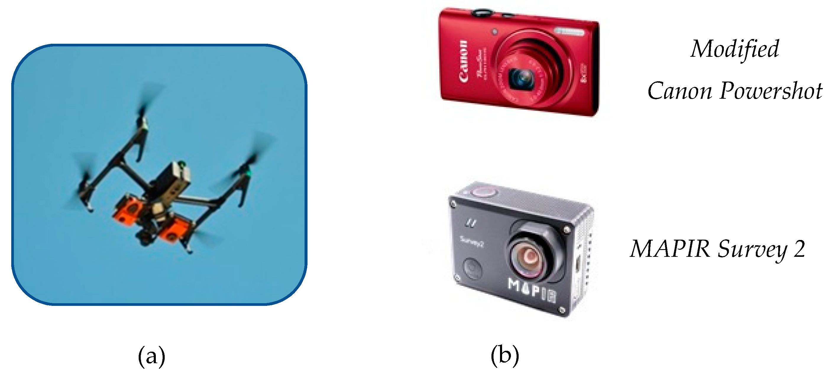
| Modified Canon | MAPIR Survey 2 | |
|---|---|---|
| Sensor resolution (pixels) | 3246 × 2448 | 4608 × 3456 |
| Focal length (mm) | 28 | 23 |
| Radiometric resolution (bit) | 24 | 24 |
| Image format | jpg | jpg |
| Image no. for Area 1 | 131 | 262 |
| Image no. for Area 2 | 154 | 324 |
| Wavebands | Red, Green, NIR | Red, Green, NIR |
| GSD (at 120 m) | 4.05 cm | 4.05 cm |
| Species | Water Treatment | Plants | Modified Canon | MAPIR |
|---|---|---|---|---|
| Buddleia (BUD) | HWS | 8 | 24 | 24 |
| LWS | 8 | 24 | 24 | |
| NS | 18 | 72 | 72 | |
| Cornus (CO) | HWS | 8 | 25 | 25 |
| LWS | 8 | 25 | 25 | |
| NS | 28 | 85 | 85 | |
| Hydrangea paniculata (HP) | HWS | 8 | 40 | 40 |
| LWS | 8 | 40 | 40 | |
| NS | 30 | 150 | 150 | |
| Hydrangea quercifolia (HQ) | HWS | 6 | 30 | 30 |
| LWS | 6 | 30 | 30 | |
| NS | 25 | 125 | 125 | |
| Physocarpus (PO) | HWS | 8 | 24 | 24 |
| LWS | 6 | 18 | 18 | |
| NS | 31 | 93 | 93 | |
| Spiraea (SJ) | HWS | 10 | 0 | 10 |
| LWS | 10 | 0 | 10 | |
| NS | 36 | 0 | 36 |
| Row | Image | Score | Stress |
|---|---|---|---|
| 1 | IMG_7696_bud_lws_729.JPG | 0.906 | TRUE |
| 2 | IMG_7695_bud_lws_815.JPG | 0.875 | TRUE |
| 3 | IMG_7694_bud_lws_644.JPG | 0.916 | TRUE |
| 4 | IMG_7696_bud_lws_730.JPG | 0.798 | TRUE |
| 5 | IMG_7694_bud_lws_645.JPG | 0.777 | TRUE |
| 6 | IMG_7695_bud_lws_814.JPG | 0.856 | TRUE |
| 7 | IMG_7694_bud_ns_658.JPG | 0.031 | FALSE |
| 8 | IMG_7696_bud_ns_747.JPG | 0.001 | FALSE |
| … | … | … | … |
| 23 | IMG_7696_bud_ns_746.JPG | 0.062 | FALSE |
| 24 | IMG_7696_bud_ns_732.JPG | 0.852 | FALSE |
| Species | Camera | Mean AUC | St. Dev | P-value | de Castro et al. |
|---|---|---|---|---|---|
| Buddleia (BUD) | Canon | 0.9931 | 0.0046 | 1.10E−05 | |
| MAPIR | 0.9907 | 0.0076 | 2.97E−05 | ||
| Cornus (CO) | Canon | 0.463 | 0.0976 | 0.2635 | |
| MAPIR | 0.5094 | 0.1661 | 0.4602 | ||
| Hydrangea (HP) | Canon | 0.6448 | 0.1381 | 0.0854 | |
| MAPIR | 0.7381 | 0.1036 | 0.0221 | ||
| Hydrangea (HQ) | Canon | 0.6639 | 0.1284 | 0.0626 | |
| MAPIR | 0.7113 | 0.1946 | 0.081 | ||
| Physocarpus (PO) | Canon | 0.8177 | 0.1759 | 0.0344 | |
| MAPIR | 0.5677 | 0.0503 | 0.0573 | ||
| Spiraea (SJ) | MAPIR | NA | NA | NA |
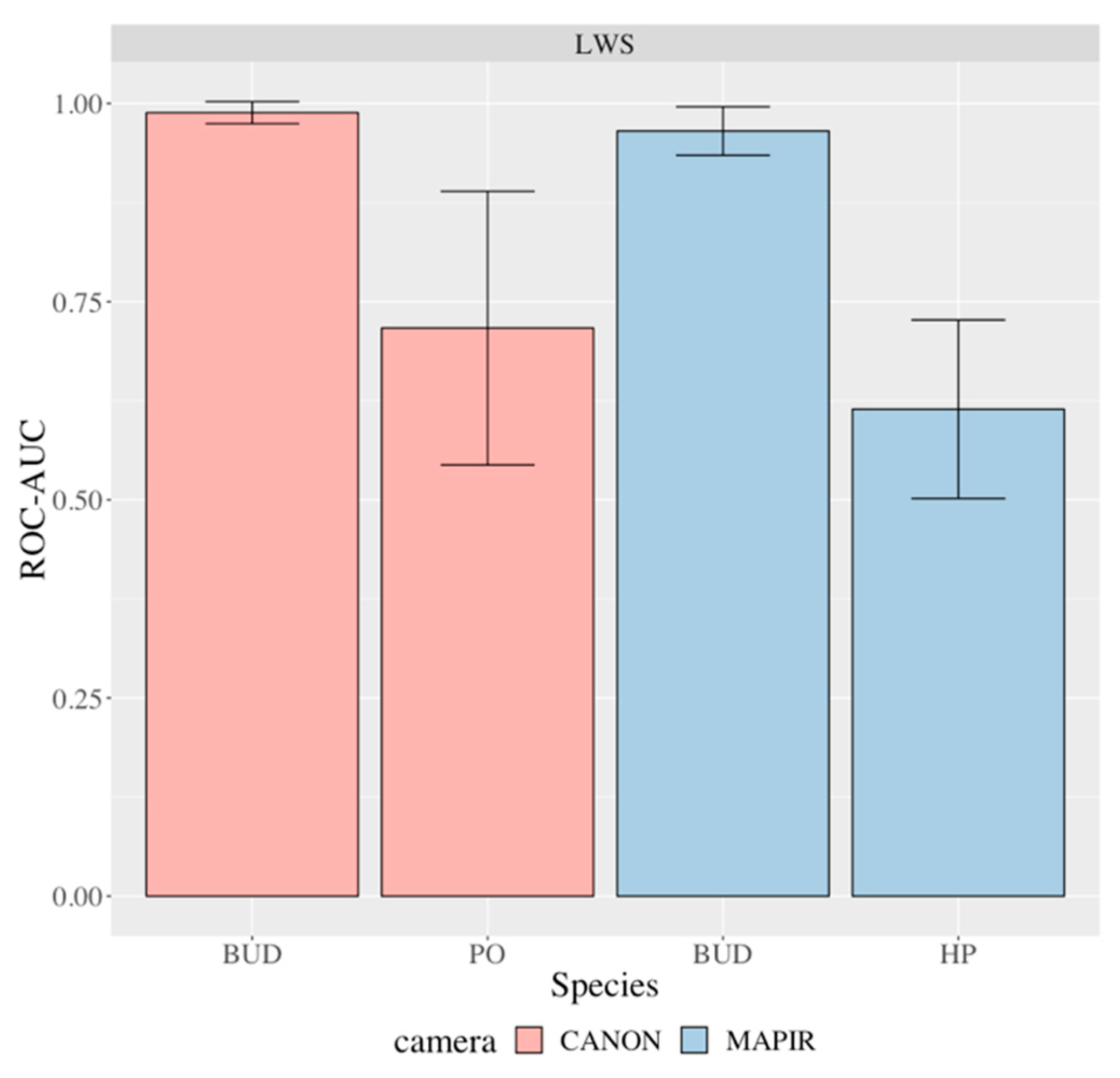
| Species | Camera | Mean AUC | St. Dev. | P-value | de Castro et al. |
|---|---|---|---|---|---|
| Buddleia (BUD) | Canon | 0.9884 | 0.0139 | 1.01E−04 | |
| Buddleia (BUD) | MAPIR | 0.9653 | 0.0306 | 5.40E−04 | |
| Hydrangea (HP) | MAPIR | 0.6144 | 0.1126 | 0.0897 | |
| Physocarpus (PO) | Canon | 0.7167 | 0.1725 | 0.0643 |
© 2019 by the authors. Licensee MDPI, Basel, Switzerland. This article is an open access article distributed under the terms and conditions of the Creative Commons Attribution (CC BY) license (http://creativecommons.org/licenses/by/4.0/).
Share and Cite
Freeman, D.; Gupta, S.; Smith, D.H.; Maja, J.M.; Robbins, J.; Owen, J.S., Jr.; Peña, J.M.; de Castro, A.I. Watson on the Farm: Using Cloud-Based Artificial Intelligence to Identify Early Indicators of Water Stress. Remote Sens. 2019, 11, 2645. https://doi.org/10.3390/rs11222645
Freeman D, Gupta S, Smith DH, Maja JM, Robbins J, Owen JS Jr., Peña JM, de Castro AI. Watson on the Farm: Using Cloud-Based Artificial Intelligence to Identify Early Indicators of Water Stress. Remote Sensing. 2019; 11(22):2645. https://doi.org/10.3390/rs11222645
Chicago/Turabian StyleFreeman, Daniel, Shaurya Gupta, D. Hudson Smith, Joe Mari Maja, James Robbins, James S. Owen, Jr., Jose M. Peña, and Ana I. de Castro. 2019. "Watson on the Farm: Using Cloud-Based Artificial Intelligence to Identify Early Indicators of Water Stress" Remote Sensing 11, no. 22: 2645. https://doi.org/10.3390/rs11222645
APA StyleFreeman, D., Gupta, S., Smith, D. H., Maja, J. M., Robbins, J., Owen, J. S., Jr., Peña, J. M., & de Castro, A. I. (2019). Watson on the Farm: Using Cloud-Based Artificial Intelligence to Identify Early Indicators of Water Stress. Remote Sensing, 11(22), 2645. https://doi.org/10.3390/rs11222645