Using Small Unmanned Aerial Vehicle in 3D Modeling of Highways with Tree-Covered Roadsides to Estimate Sight Distance

Abstract

The safe and efficient operation of highways largely depends on the adequate provision of sight distance. Small unmanned aerial vehicles (UAVs) can be utilized to efficiently complete data acquisition very soon after identifying an issue when searching for potential highway safety risks. A double grid flight is proposed to obtain an adequate three-dimensional (3D) recreation of the road environment, ensuring an unbiased sight distance output. Then, a dense cloud point is derived through a Structure from Motion Multi-View Stereo process. The point cloud is classified to produce both a terrain model, characterized by its resolution, and a 3D-object model, characterized by the maximum edge length of the entities. The resulting road environment model is utilized to calculate sight distance in a geographic information system. The results enabled the detection of accident-prone locations caused by sight distance limitations. Moreover, the impact of the 3D modeling parameters on the results was assessed.

1. Introduction

The safe and efficient operation of highways largely depends on the adequate provision of sight distance throughout their lifespan. To examine the current state of in-service facilities, efficient data collection techniques are required. Where local sight distance issues arise, small unmanned aerial vehicles (UAVs) are an effective solution that can contribute to reducing costs in surveying, as they are economical tools while providing highly valuable data. The current development and popularization of this technology facilitates highway administrators to complete the data acquisition very shortly after identifying an issue. This contributes to giving a quick diagnosis and to decision-making in order to solve the identified problem. An additional advantage of this equipment is that the data collection produces no interference with the operation of the infrastructure. However, the presence of dense vegetation or tree crowns overhanging the roadway might mask relevant features for the analysis. Therefore, the data collection procedure must be designed to adjust in order to comply with the requirements of the final purpose.

This paper presents a methodology for the study of highway sight distance based on the data collected by a small UAV platform. Data acquisition was carried out by the aircraft following a double grid trajectory. Next, a road environment model was built up, consisting of a Digital Terrain Model (DTM) and a three-dimensional (3D) model of the objects by the roadsides. In addition, the effect of both the DTM resolution of and the 3D object modeling features on the sight distance output is analyzed.

2. Background

Small UAVs are commonly equipped with a camera capable of capturing high-resolution images and recording videos. This equipment provides them with great versatility, making them suitable for a wide variety of applications. These benefits have been acknowledged by several studies related to terrain modeling [1,2]. The capabilities of UAV-based systems have also been utilized to survey earthwork projects [3]. These applications of UAVs can likewise be found in the field of highway engineering. Carvajal et al. [4] characterized landslides on road ditches through photogrammetry. UAV-based digital imaging systems are capable of collecting surface condition data to characterize unpaved roads [5,6]. UAV platforms have also been used to measure road surface deformation with high accuracy [7]. Feng et al. [8] extracted highway geometry features from a UAV mapping system. Several studies have used UAVs for tracking traffic operations. Vetters and Jaehrig [9] recorded passing maneuvers using a UAV to model passing sight distance on two-lane rural highways. Zhang et al. [10] devised a real-time traffic incident detection system based on video recording from a UAV. Salvo et al. [11] extracted kinematic data of traffic in urban environments utilizing a UAV system.

Digital photogrammetry techniques based on Structure from Motion Multi-View Stereo (SfM-MVS) process is an efficient image-based method that allows to recreate real world scenes [12]. The images acquired by UAV systems make it possible to obtain geospatial products of special interest in engineering applications. Common tie points are detected and matched on photographs so as to compute both the external and internal camera orientation parameters for each image [13]. Based on the estimated camera positions and orientation in the 3D space, the depth information of the point is derived by taking account of the camera position estimates where such points are identified. The process combines the depth information from all points into a single dense point cloud.

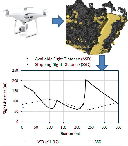
The available sight distance (ASD) is defined as the distance between the driver’s position and the furthest target seen without interrupting the sightline, with this being measured along the vehicle’s path. The evaluation of sight distance requires recreating the highway and its roadsides. A 3D recreation is more likely to produce accurate results than as-built 2D drawings for two reasons. First, the spatial combination of the highway alignments and features in different projections gives rise to a new reality. Second, the 3D recreation enables the incorporation of updated data of the current state of facilities.

The recreation of the shape of a highway requires several inputs. UAVs are capable of generating highly accurate digital models, which are entities defined in space that represent the elevation of an area [14]. Whereas digital terrain models (DTMs) represent the bare ground surface, digital surface models (DSMs) reproduce additional surfaces on the terrain such as vegetation or buildings. Several procedures have been devised in geographic information systems (GIS) to assess sight distance on existing highways, which reproduce the DTM by means of a either a raster file [15,16] or a triangular irregular network [17].

Currently, the most used sources from which digital models can be derived involve the use of Light Detection and Ranging (LiDAR) equipment or photogrammetry. Bassani et al. [18] modeled urban environments using a mobile mapping system from which the shape of 3D objects was derived using photogrammetry.

A univocal relationship must exist between every position on the horizontal projection of a model and its elevation. Several authors have discussed the difficulties inherent to this characteristic as overhanging structures yield nonexistent hindrances [19,20]. Charbonnier et al. [21] evaluated highway sight distance on 3D models consisting of triangular faces built up from a LiDAR point cloud. An alternative procedure for elaborating virtual 3D models of existing highways and roadside features was devised and validated for evaluating of sight distance [22,23]. It used a DTM combined with a fully 3D-defined structure to model objects, overcoming the difficulties of DSM to adequately represent overhanging features. Jung et al. [24] evaluated sight distance at urban intersections where, in addition to a DTM, existing 3D objects were reproduced by means of voxels. Voxels are regions of space, generally cubes or spheres, which are assumed to be occupied in reality by part of an object based on the fact that at least a surveyed point is located in it.

Other procedures not relying on creating surfaces but on the raw LiDAR point cloud instead were proposed to estimate sight distance on highways [25], although this procedure is potentially biased, as sightlines might slip between points in low-density areas. To overcome such issues, Ma et al. [26] developed a procedure that estimated sight distance on a raw point cloud by means of a sight cone, where a triangulation algorithm connected the points lying inside the cone to recreate the objects in the road environment.

Diverse authors sought to characterize the effect of the quality of a model on visibility. Ruiz [27] examined the effect of DTM error on an estimate of viewshed. Kloucek et al. [28] used random control points to confirm that a model with higher resolution enables a more accurate sight distance output. Castro et al. [29] described the impact of DTM resolution and the spacing between path stations on highway sight distance studies.

3. Materials and Methods

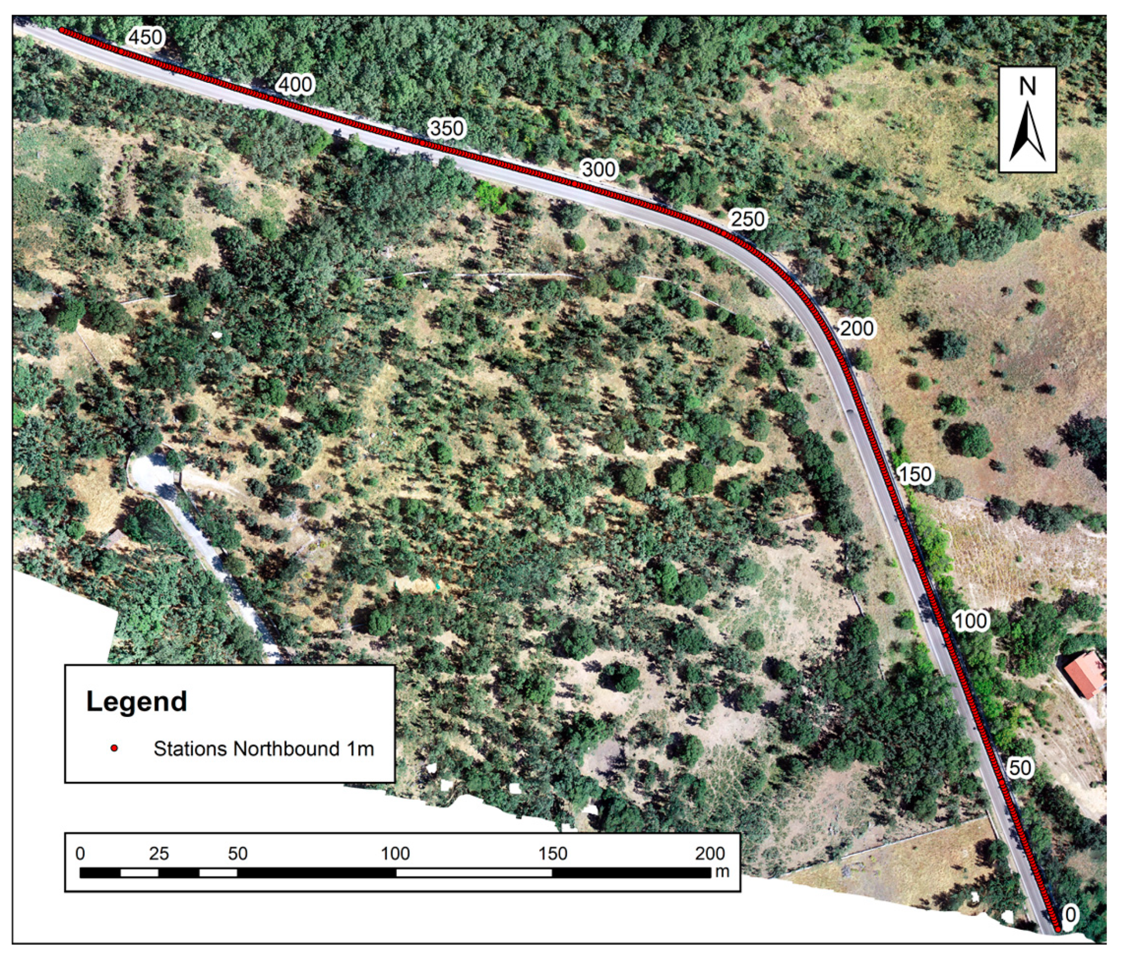
A two-lane rural highway segment was selected to test the methodology hereby proposed. It is located in the region of Madrid (Spain) and traverses a rolling terrain. The length of highway covered by the area surveyed in a single flight was 1400 m, from which a subsection of approximately 470 m was selected to perform the study (Figure 1). It features a horizontal curve of radius 75 m and crest vertical curves whose parameters are 365 and 725 m. In addition, three accidents with injured were produced over a period of 7 years. The highway cross section features a composite profile, and the roadsides have leafy vegetation, which may significantly reduce the ASD.

The Phantom 4 PRO UAV platform was used to survey the highway segment and its roadsides. It is a quadcopter equipped with Global Positioning System (GPS) and Inertial Measurement Unit (IMU) modules for autonomous navigation and further imaging geotagging. The platform includes a non-metric RGB camera with a CMOS active pixel sensor technology.

Table 1. Technical specifications of the multirotor UAV platform used.

Aircraft Feature	Specifications
Model	Phantom 4 Pro
Weight (include battery + sensor)	1388 g
Flight Range	4.3 mi/7 km
Max speed	31 mph/50 km/h (mode P)
Max wind resistance	10 m/s
Maximum flight time	30 min

shows the technical characteristics of the platform and

Table 2. Technical specifications of the camera sensor used for imagery acquisition.

RGB Camera Feature	Specifications
Sensor	FC6310 - 1’’ CMOS
Lens	FOV 84° 8.8 mm/24 mm (35 mm format equivalent) f/2.8 - f/11 auto focus at 1 m-∞
Image sensor resolution	5472 × 3648 pix
Focal length	8.8 mm
Sensor size	13.2 × 8.8 mm

the sensor features.

Data collection was planned before flying the UAV. The flight planning was aided by freeware PIX4D capture [30], as seen in Figure 2. The target ground sample distance (GSD) for the images was 2 cm/pixel, which resulted in a theoretical flight height of 72 m above ground level.

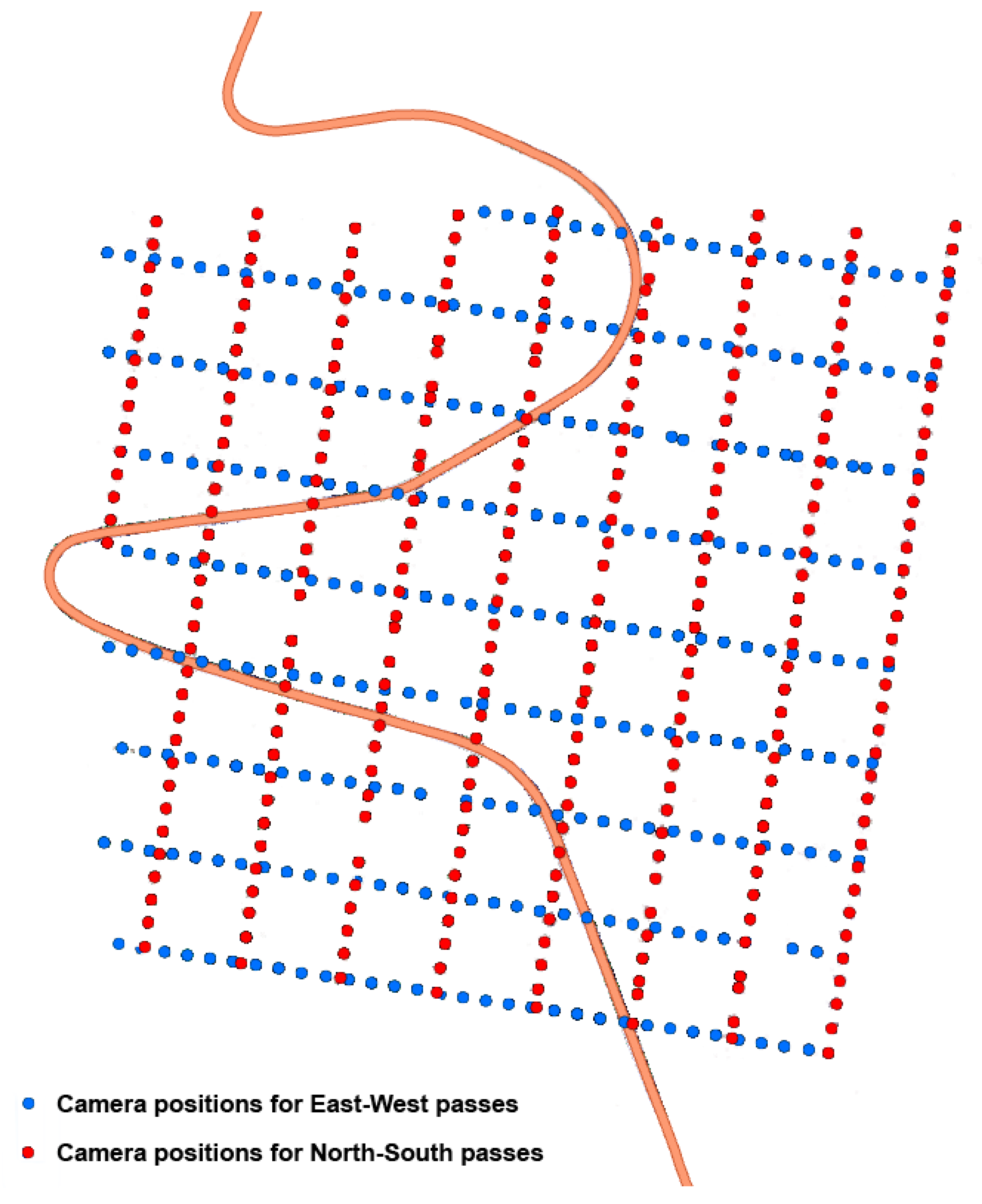
A double grid trajectory was selected for the survey, the UAV platform completing first the lines in one direction and then the lines in the perpendicular direction as illustrated in Figure 2. Due to the high overlaps from different viewing angles, this flight pattern is the most suitable one to recreate 3D scenarios by photogrammetric methods as it maximizes the survey coverage [30]. This facilitated the recreation of overhanging features as well as the terrain below. It must also be noted that the grid orientation did not follow the highway alignment of the surveyed section.

The flight planning also involved the analysis of local risks to ensure that the flight could be carried out under safe conditions. After inspecting the flight area and selecting a safe take-off and landing site, an on-site preliminary inspection of the platform was carried out to rule out in-flight loss of control. At the take-off of the equipment, it rose to the scheduled height above the ground, remaining at that height throughout the flight. Therefore, the flight height above the ground varies with each shot.

The operating platform included the UAV and the camera sensor, both operating fully autonomously and controlled by autopilot. The flight was executed in accordance with the local UAV regulations and was also managed by PIX4D capture software.

The equipment acquired a total of 585 images, which were taken at an average height of 75.1 m due to the natural undulation of the terrain.

Table 3. Technical specifications of flight planning.

UAV Flight Feature	Specifications
Type	Double grid
Area	668 × 736 m
Overlapping	80% front/40% side
Average flight height	75.1 m
Ground sample distance	2.04 cm
Total flight length	18,657 m

summarizes the technical parameters of the UAV-based survey.

Agisoft PhotoScan® Professional v. 1.5.1, one of the most common SfM-MVS software suites, was used to obtain the cloud point and the orthomosaic [31]. The photogrammetric products obtained from the acquired images were the dense point cloud and the orthomosaic. These two basic products were required for the subsequent sight distance analysis. The application of the SfM-MVS process requires the insertion of a scale, and data orientation with respect to the north and the vertical, to enable the measurements of geometric features and orientations [32]. In this sense, control point coordinates (x, y, z) of surface features were determined from the mosaic of the latest orthophotographs and DTM available from the National Geographic Institute of Spain (IGN) in ArcGIS [33]. Control points located on plain terrain and easily recognizable on the images were selected.

Table 4. Technical results for the Agisoft PhotoScan imagery process.

UAV Survey Output Features	Specifications
Number of images	585
Camera stations	578
Ground resolution	2.04 cm/pix
Coverage area	0.32 km2
Reprojection error	0.26 pix
Cloud point density	880 points/m2
Number of images	585

shows the technical specifications of the final output for the SfM-MVS process.

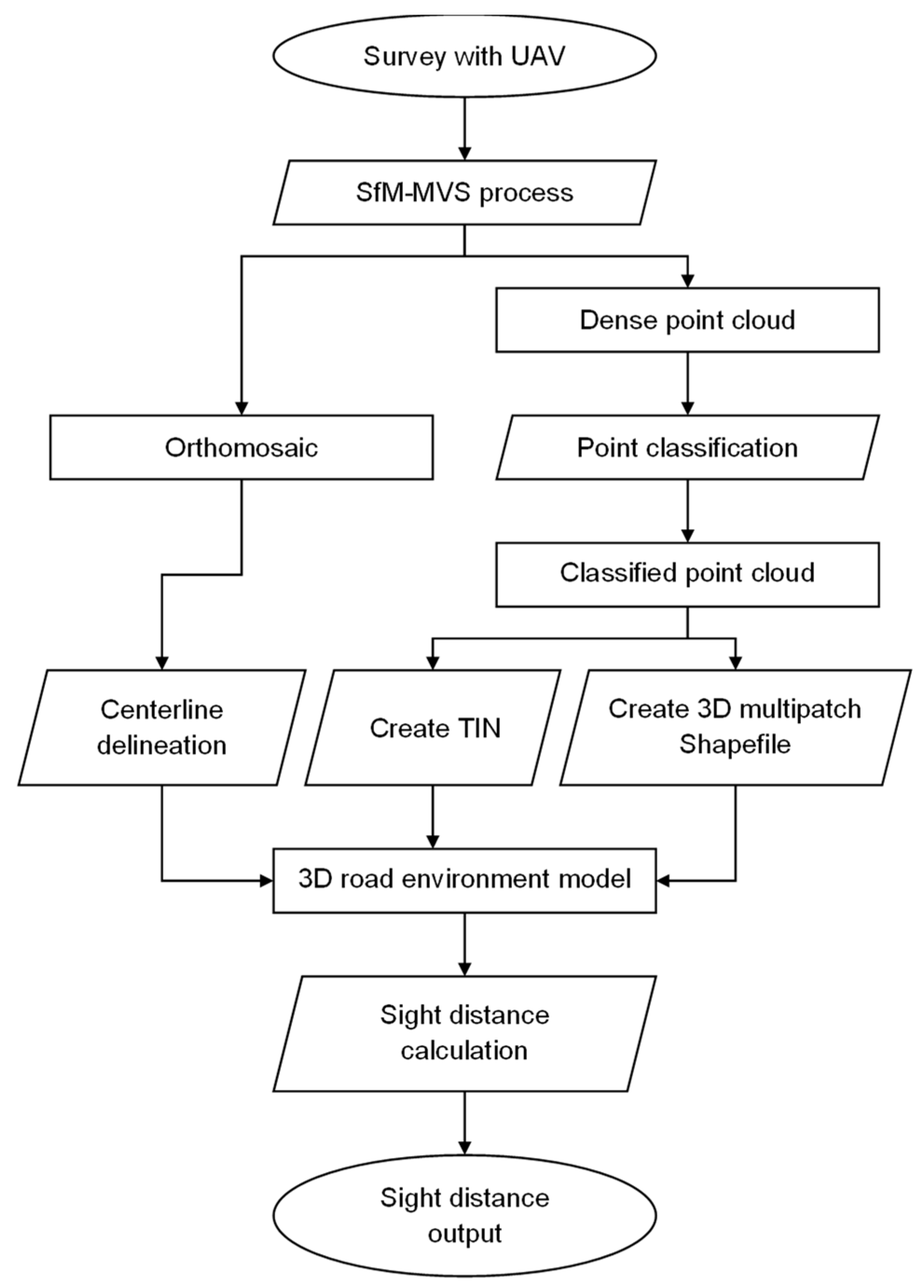
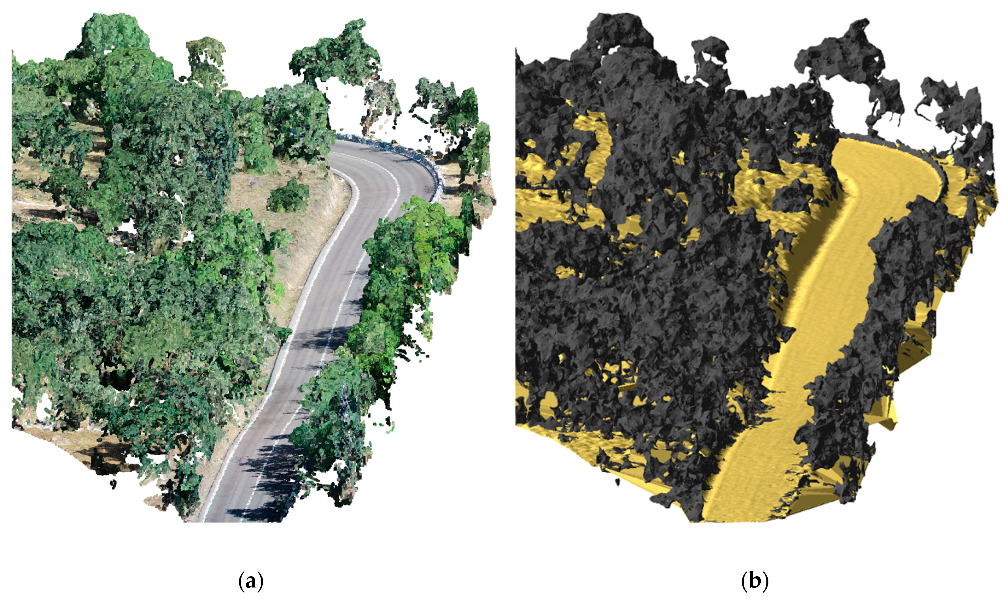
The data processing workflow and the sight distance estimation are outlined in Figure 3. First, the output produced by the UAV survey underwent the SfM-MVS process. An orthomosaic and a dense point cloud in LAS format were derived from this process. As can be seen in Table 4, the resolution of the orthophotograph obtained was 2.04 cm/pix, while the reprojection error was 0.26 pix. Figure 4a displays the colored point cloud in an area surrounding the highway studied. From here on, the workflow unfolds in two processes. On the one hand, the orthomosaic was used to derive the horizontal projection of the highway centerline and, from this, two point shapefile vehicle paths, one per travelling direction, were created in ArcGIS Desktop assuming a fixed centerline offset of 1.5 m, as per the Spanish geometric design standard [17,34]. The path stations were spaced 1 meter apart, along which both the observer and the target were to be placed. Although this is the default configuration, the procedure allows the target position to be set flexibly [22].

On the other hand, software MDTopX was selected to classify the dense point cloud [35]. The aim of this classification was to organize the LAS points into different categories, which will serve to create detached elements of the 3D road environment model. Standard LiDAR classification codes were defined by the American Society for Photogrammetry and Remote Sensing (ASPRS) [36]. Three standard LiDAR point classes were considered: “unassigned”, “ground” and “high vegetation”. Except for the “ground” class, the other two classes were not intended to represent accurately which type of element the point captured belonged to, but to serve to create the features required to model the highway and its roadsides with the maximum possible point density. Moreover, assigning the correct class to non-terrain points is not as important as identifying the spatial position of the potential visual obstruction. It should also be noted that points corresponding to mobile obstacles such as traffic were identified and removed. Then, a point shapefile was created in ArcGIS from the ground points, which served as input to produce a triangular irregular network (TIN) dataset. In parallel, a 3D multipatch shapefile was created in MDTopX from the points classified as “unassigned” and “high vegetation”, which were computed using a 3D Delaunay triangulation algorithm [37]. A multipatch feature is an ArcGIS object that stores a collection of patches (generally triangular) to represent the boundary of a 3D object [38]. A multipatch shapefile may consist in turn of one or several features. A TIN dataset and a multipatch shapefile, both derived from the dense cloud point, are shown in Figure 4b.

The 3D model recreating the highway and its roadsides is built up in ArcGIS once the vehicle paths, the TIN dataset and the multipatch shapefile have been incorporated. The two former datasets are necessary inputs, while the latter is optional for launching the sight distance geoprocessing model for ArcGIS developed by the authors [23], which assembles several tools of the ArcToolBox. This procedure connects stations on the point shapefile that represents the vehicle path. These stations are assigned an elevation above the DTM according to an attribute. When the station is considered to be the origin of the sightline, the value of the attribute to be given is the observer’s eye height. Otherwise, the corresponding attribute is the target height. In this study, the values of these attributes were set constant according to the current specifications in the Spanish highway geometric design standard [34], which are 1.1 and 0.5 m, respectively. Another important attribute of stations is their distance to the origin, measured along the path itself. Only sightlines which connect observers located at a station closer to the origin than the target are selected for the sight distance evaluation, meaning that a driver needs to perceive the information of the immediate section ahead. Moreover, the user can select the maximum distance between the observer and the target in the analysis. For every sightline, the algorithm checks whether the DTM or the multipatch shapefile produce a visual obstruction. The output of the sight distance analysis comprises several ArcGIS features. First, the evaluated sightlines divided into visible and non-visible segments. It must be noted that, when the sightline was obstructed by either the terrain or a multipatch 3D object, two segments were obtained, whereas the whole sightline is obtained if otherwise. In addition, a point feature class is produced, indicating the positions where the visual obstructions intercepted the sightlines.

4. Road Environment Modeling

To recreate the roadway environment of the case study, a DTM dataset in the shape of a TIN was first generated from all the points of the dense point cloud classified as “ground”. Given that the dense point cloud comprised 880 points per m², it can be deduced that on areas where points were exclusively classified as “ground”, the derived TIN connected nodes at an approximate distance of as close as 3 cm. In addition, to further evaluate the impact of the DTM resolution on sight distance modeling, five more TIN datasets were also generated from the “ground” points of the dense point cloud. Each TIN dataset featured a different resolution, i.e., the distance between connected points, called nodes. For these five datasets, the terrain model was customized by means of a generalization carried out in MDTopX. In the former case, the points presented a scattered layout since the original points were directly utilized. In each of the latter cases, the area covered by the point cloud was divided into a grid of squared tiles, whose side was selected at 0.1, 0.2, 0.5, 1 and 2 m. The DTM generalization consisted of assigning a unique elevation value to each tile equal to the average elevation of all the points that lied on the tile. Then the TIN nodes had the coordinates of the center of the tile with the corresponding elevation assigned. As a result, the output set of generalized ground points followed a grid pattern.

Four Multipatch shapefiles were likewise generated. The parameter that features these 3D datasets is the diameter of the sphere in the 3D triangulation algorithm, in other words, the maximum edge length of the polyhedral entities produced. This parameter is closely linked to the 3D shape of the objects to be modeled and its value has, therefore, a double effect in the accuracy of modeling 3D objects [37]. On the one hand, too long a maximum edge length will produce large faces that might create non existing occlusions. This issue is nonetheless assumed to be prevented to some extent with the point classification since the 3D triangulation algorithm only connects points belonging to the same class. For example, points of tree crowns would not be connected with ground points even for large maximum edge lengths whereas points belonging to the same class would. On the other hand, too short a length, particularly below the point density of the area, would prevent faces from being created, missing some object features. As opposed to the characterization of the DTM from the 2D density of the point cloud, the 3D density of the point cloud does not have such a straightforward relation to the characterization of the 3D object modeling. The point density tended to be concentrated on the 3D surface of the object instead of being scattered in space. Nonetheless, although not comparable, regions of space where the dense point cloud represented tree crowns and other 3D objects typically reached densities greater than 1,000 points per m³, a value that may be used as a reference. Yet it should be borne in mind that as the maximum edge length decreases to feature very fine details, larger datasets are created, which increases sight distance computation time. It should also be noted that points that correspond to vegetation might be affected by a certain level of noise. A balance between point cloud density and the computing performance should be achieved. Therefore, the selected maximum edge lengths were 0.2, 0.5, 1 and 2 m.

A reference 3D model of the highway was built up incorporating the full-size TIN dataset and the multipatch featured by the 0.2-m maximum edge length to assess sight distance on the selected section on both driving directions. Moreover, highway models comprising all the possible combinations of TIN datasets and multipatch shapefiles were contemplated, which yielded 24 models of the road environment to evaluate the impact of dataset parameters on the 3D model. Figure 4b displays the road environment model that incorporated the TIN dataset with 0.2 m grid size and the multipatch shapefile with maximum edge distance of 0.5 m. Provided that both driving directions were examined on the selected highway section, a total of 48 sight distance series were launched. Nevertheless, the ASD series corresponding to the same highway model were merged. In addition, the ASD values at stations where equaled the distance to the last station in any of the series were removed from the sample. Then a total of 718 ASD values comprised each series.

5. Results and Discussion

As mentioned earlier in this paper, the ASD was calculated on 24 different 3D models of the highway section studied. To analyze the results, the ASD outcome for the outward direction of two 3D highway and roadside models are presented in Figure 5. The ASD outcome in the reference model (the TIN with all terrain points and the multipatch shapefile with maximum edge 0.2 m) is displayed with a solid black line, and the outcome in the 3D model with the 2-m grid TIN and the 2-m maximum edge multipatch is displayed with a solid grey line. Although both series remain close to each other, it can be noticed that the one with the greater parameter values over- and underestimated the ASD with respect to the reference model. In particular, the station where a sudden increase of ASD was produced varied from model to model at the beginning of the section studied.

To assess the safety features of the section studied, the ASD was compared to the required stopping sight distance (SSD), which is represented by the dashed line in Figure 5. The SSD is the standard distance needed by a driver forced to stop a vehicle as quickly as possible. The SSD values were computed at each station as per Equation (1), provided by the Spanish geometric design standard [34]:

$$SSD=\frac{V·PRT}{3.6}+\frac{V^2}{254·\left(f_l\pm g\right)}$$

(1)

In Equation (1), V is the speed at which a driver is supposed to drive according to an operating speed profile built up as per the geometric features of the section [39,40,41]. To build up the operating speed profile, the vehicle is considered to travel at a constant speed on curves, while it decelerates when approaching and accelerates when exiting, both being performed at variable rates. PRT is the perception and reaction time, i.e., the time that elapses between the moment the driver first sees a hazard on the roadway and the moment they apply the brakes. f_l is the longitudinal friction between the tire and the pavement. g is the grade on the vertical projection of the line that connects the initial stopping station and the station at which the vehicle has stopped completely, positive if uphill and negative if downhill.

By examining the results illustrated in Figure 5, potential sight distance issues are indeed identified. A local minimum is found in ASD around station 100, which is caused by a tight crest vertical curve. Another local minimum is located around station 200, which is caused by the limited sight distance on the horizontal curve displayed in Figure 1. These results highlight that the method used is capable of finding and identifying sight distance restrictions in 3D, which may be caused by features of either the horizontal or the vertical projection. In both local minima, the ASD do not meet the required SSD, thus creating accident-prone locations. The ASD deficit in the case of the crest curve extents between stations 70 and 125, becoming particularly severe as the difference reaches up to 40 m. In addition, the ASD limitation while approaching the horizontal curve, which extends for 70 m, could prevent drivers from recognizing it. It is worth noting here that no signals exist to warn drivers about zones with limited ASD or reduced posted speed. To promote the safe operation of traffic, a posted speed of 50 km/h would need to be enforced in the section, according to Equation (1).

A two-way repeated measures analysis of variance (ANOVA) test was conducted in the statistical software suite SPSS to evaluate whether the DTM resolution and the maximum edge length in 3D object generation affected the sight distance outcome. The number of subjects was set to be equal to the 718 positions from which the ASD was evaluated, and each one had 24 ASD values associated from the respective highway 3D model explained above. This analysis required the adjustment of a generalized linear model, which included the two aforementioned factors, as well as the interaction term. Pillai’s trace test of significance was used to evaluate the impact of the factors on ASD modeling. The outcome is the Pillai’s trace statistic, which is a positive value ranging from 0 to 1. Increasing values of the statistic indicate effects that contribute more to the model. Accordingly, the interaction factor has a greater effect on the ASD outcome than the other two factors as displayed in

Table 5. Results of the two-way repeated measures ANOVA test.

Factor	Pillai’s Trace Value	F-Statistic	Significance
DTM resolution	0.038	5.709	<0.001
Multipatch maximum edge length	0.077	19.760	<0.001
Interaction	0.130	7.005	<0.001

. The maximum edge length in turn had a greater effect on the ASD outcome than the DTM resolution in the case study. Moreover, it can be concluded at the 99.9% confidence level that the two factors and their interaction significantly affected the ASD outcome.

Figure 6 shows the Profile Plot for interaction effect DTM resolution–multipatch maximum edge length. This chart includes the estimated marginal means and the boundary intervals, for a 95% confidence level.

6. Conclusions

This study has demonstrated the benefits associated with the use of UAVs in data acquisition of highway sections that might present road safety issues. While this equipment facilitates highway administrators in completing data collection very soon after identifying safety issues, it is capable of providing accurate enough data for the purposes of 3D road environment modeling at a moderate cost in comparison to other data sources. In this sense, the main novelty is that the data captured by the UAV platform is used to create a 3D model of the road and its environment that is adequate to assessing sight distance on a highway section.

The double grid layout of the UAV flight enabled sufficient coverage of the area of interest to obtain a dense cloud point through the SfM-SVM process, which served to recreate the road environment by means of a TIN dataset and a 3D object file. This procedure enabled the recreation of overhanging features adequately.

In the case study presented, sight-distance-related safety issues were identified and the zones where they are produced were characterized. Consequently, it was concluded that the observed sight distance limitations might be a relevant factor in the safety performance of the highway section, and countermeasures may be proposed for solving the problem. Highway administrators could propose increasing the clearance by the curve roadside, reducing the posted speed, or even redesigning the alignment on the hazardous section.

From a qualitative point of view, the ASD results yielded by the different highway 3D models produced similar results, although evident differences were observed. Moreover, statistical tests were carried out to assess the effect of the parameters characterizing the 3D model on the sight distance output. It was found that the resolution of the DTM significantly affected the accuracy of the ASD outcome. Therefore, it is recommended that a DTM with the finest possible resolution be used for the purposes of ASD analysis. Moreover, the maximum edge length of the 3D multipatch features, as well as the interaction with the aforementioned factor, also significantly affected the ASD accuracy. In the case of this input, point classification is acknowledged to enhance the features of 3D object modeling. It is, therefore, recommended that the finest possible size enabled by the 3D density of the point cloud be selected. In the present study, a reference value of the DTM resolution would correspond to 0.1 m and, in the case of the maximum edge length of the 3D multipatch features, it would correspond to 0.2 m.