Article

Evaluation of Incident Light Sensors on Unmanned Aircraft for Calculation of Spectral Reflectance

by
E. Raymond Hunt, Jr.
* and
Alan J. Stern
USDA-ARS Hydrology and Remote Sensing Laboratory, Beltsville Agricultural Research Center, 10300 Baltimore Avenue, BARC-West Building 007 Room 104, Beltsville, MD 20705, USA
*
Author to whom correspondence should be addressed.
Remote Sens. 2019, 11(22), 2622; https://doi.org/10.3390/rs11222622
Submission received: 28 September 2019 / Revised: 30 October 2019 / Accepted: 6 November 2019 / Published: 9 November 2019

Abstract

:
Including incident light sensors (ILS) with multispectral sensors is an important development for agricultural remote sensing because spectral reflectances are necessary for accurate determination of plant biophysical variables such as leaf area index and leaf chlorophyll content. Effects of different aircraft flight conditions on accuracy of surface reflectances retrieved using an ILS are not known. The objectives of this study were to assess the effects of ILS orientation with respect to sun and aircraft altitude. A Tetracam Miniature Multiple Camera Array (Mini-MCA) was mounted on a fixed-wing unmanned aircraft system (UAS) with the ILS mounted on top of the aircraft’s fuselage. On two dates the aircraft flew over six 50-ha agricultural fields with center-pivot irrigation at three different altitudes (450, 650 and 1800 m above ground level (AGL)). Ground reflectances were estimated using atmospherically corrected Landsat 8 Operational Land Imager data acquired at or near the time of the aircraft overflights. Because the aircraft had a positive pitch during flight, the ILS pointed opposite to the flight direction. The first date had flight lines closely oriented towards and away from the sun. The second date had flight lines oriented perpendicularly to the solar azimuth. On the first date, red and near-infrared (NIR) reflectances were significantly higher when the ILS was oriented away from the sun, whereas ILS orientation had little effect on the second date. For both dates, red and near-infrared reflectances were significantly greater at 450 m compared to 1800 m. Both the effects of ILS orientation and flight altitude are correctable during image processing because the physical basis is well known.

Graphical Abstract

1. Introduction

Remote sensing from unmanned aircraft systems (UASs, also called unmanned aerial vehicles, remotely piloted aircraft, or drones) has become important for searching agricultural fields for problems, which are then verified on the ground by crop scouts [1,2]. Furthermore, UASs may provide remotely sensed data required for planning variable-rate applications of water, fertilizers, pesticides and herbicides when, where, and with the amount required to maintain crop yields while minimizing excess applications [1,2,3,4,5]. In general, these applications require surface spectral reflectances for accurate implementation of the algorithms [6,7].
The sensors mounted on UASs need to have low weight. As a result, image quality may be inadequate for the application, and radiometric calibration is therefore a critical step [8,9]. Recently, multispectral sensors made for UASs have included incident-light sensors (ILSs, also called irradiance sensors or downwelling-light sensors) for correcting surface radiance or luminance to reflectance [2]. There have been some studies on the accuracy of radiometric corrections using an ILS [10,11,12,13]. A big concern is changing the incidence angle between the sun, target and sensor where changes in reflectance occur as a result of the target’s bidirectional reflectance distribution function (BRDF) [14,15,16,17,18]. ILSs and sensors are assumed to be level when mounted on an aircraft, but changes in aircraft attitude (roll, pitch, yaw) and solar position (zenith angle and azimuth) affect sensor and ILS orientation with respect to the sun [19,20,21]. Our first objective was to assess the relative contributions of BRDF and ILS orientation on retrieved spectral reflectances.
In many countries, laws and regulations restrict UAS flight altitudes below a range of 90–150 m above ground level (AGL), so seldom is altitude considered as there is little change in retrieved reflectance [18,22]. However, UAS flights at greater altitudes may be allowed with special permission from civil aviation authorities on a case-by-case basis. The U.S. Federal Aviation Administration is developing plans to fully integrate UASs with manned aircraft into the nation’s airspace [23], which may allow flights at higher altitudes without special permission. With much higher altitudes, there is more atmospheric scattering between the ground and sensor, which would increase path radiance, but decrease direct radiance from the target. Because it is not known how high altitudes will affect UAS remote sensing, our second objective was to analyze these effects by atmospheric modeling and experimentation.
There is an enormous variety in the types of UASs flown. Multirotor vertical take-off and landing UASs, such as quadcopters, are used frequently for acquiring remotely sensed data over agricultural fields. These aircraft are relatively stable during flight. Compared to fixed-wing UASs, multirotor UASs have limitations on altitude, air speed and flight duration, and thus may only cover small fields within a reasonable amount of time. Therefore, fixed-wing UASs may become necessary to cover large fields, but fixed-wing UASs will have larger changes in aircraft attitude, namely the aircraft’s roll, pitch and yaw. Based on our objectives, we tested two hypotheses: (1) that the incidence angle between the sun and the ILS is the primary variable affecting retrieved reflectances, and (2) that increases in altitude reduce the retrieved surface reflectance using an ILS. These two hypotheses were examined using a low-altitude long-endurance fixed-wing unmanned aircraft [24]. Because the study area was large (greater than 5 km2), we used imagery from the Landsat 8 Operational Land Imager (L8-OLI) to serve as independent ground data.

2. Methods

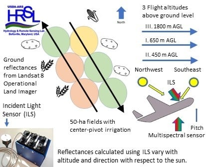
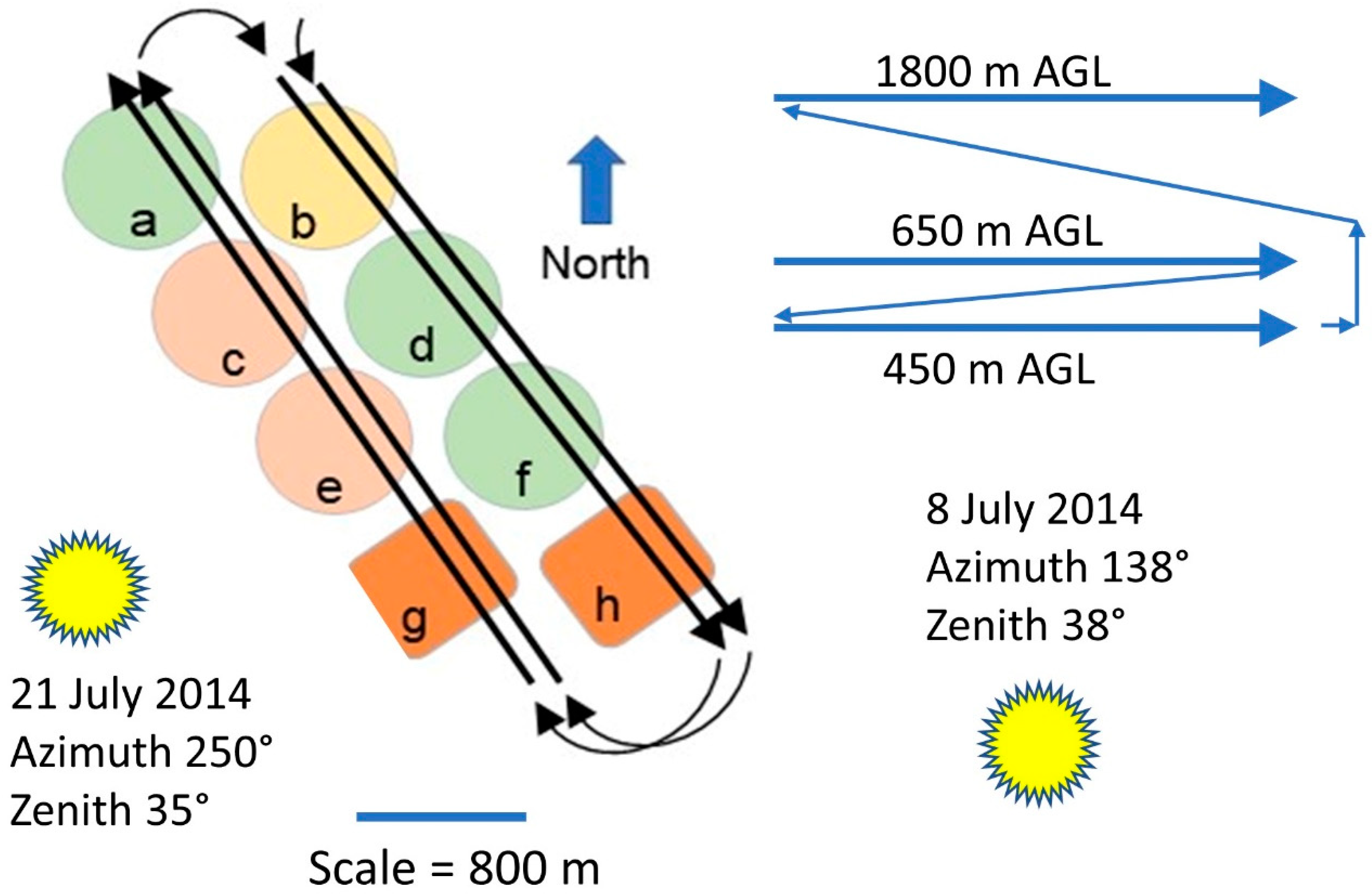
2.1. Experimental Design and Flight Plan

The experiments were conducted during the summer of 2014 in a region of irrigated agriculture located in the Columbia River Valley in north-central Oregon, USA (at about 45.7° N latitude, 119.9° longitude, and a 215-m elevation above mean sea level). Six center-pivot-irrigated fields were selected, each with an area of 50 ha (Figure 1). According to the U.S.D.A. National Agricultural Statistics Service 2014 Cropland Data Layer [25], the crops were: three fields of potato (Solanum tuberosum), one field of maize (Zea mays), and two fields of spring wheat (Triticum aestivum). The spring wheat was harvested, so the fields were mostly bare soil and crop residue. To extend the range of apparent surface reflectance, two areas of untilled sagebrush steppe directly south of the fields were used. The dominate species were Artemisia tridentata and Bromus tectorum. The total study area was 5.3 km2.
A low-altitude long-endurance fixed-wing unmanned aircraft was used to conduct flights at three altitudes on two different days, 8 July and 21 July 2014 (Figure 1). The southeastern flight lines always had a bearing of 150°, whereas the northwestern flight lines always had a bearing of 330°. The 8 July flight was conducted at 9:30 a.m. Pacific Daylight Time, so the flight lines were nearly aligned with the solar azimuth (Figure 1) and aircraft pitch angles were expected to have a large effect. The 21 July flight was conducted at 2:00 p.m. hours, so the flight lines were nearly perpendicular to the solar azimuth and aircraft pitch was therefore expected to have little effect (Figure 1). Three altitudes were covered with each flight: first at 650 m, then at 450 m, and finally at 1800 m AGL. Total flight time to cover the study area at all three altitudes was about 70 min. The airspace above the fields was a Military Operations Area controlled by the U.S. Department of Defense; thus, U.S. Federal Aviation Administration rules for commercial UASs (altitude < 120 m) were not applicable.

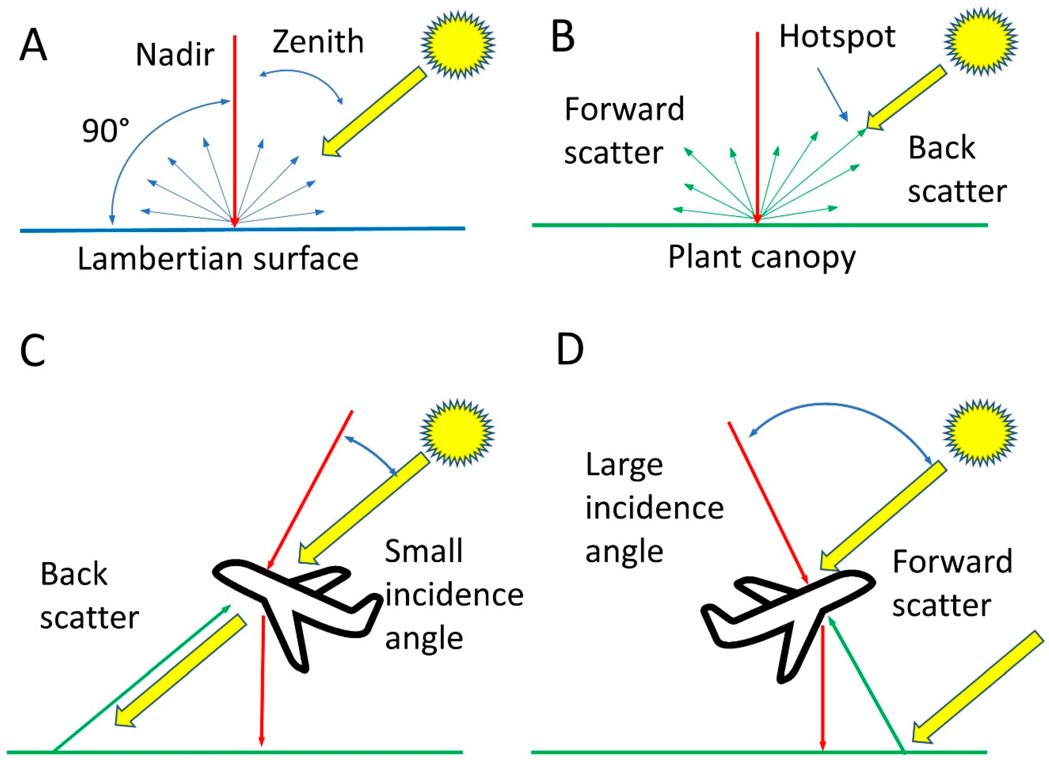
2.2. Effect of ILS Orientation on Retrieved UAS Reflectance

A Tetracam, Inc. (Chatworth, CA, USA) six-channel Miniature Multiple Camera Array (Mini-MCA) was used with five filters (Table 1): blue (470 nm), green (550 nm), red (660 nm), red-edge (710 nm), and near-infrared (810 nm). For each of the five bands, the sensor’s pixel size was 5.2 µm, and the lens focal length was 8.5 mm. Image size for each channel was 1240 columns by 1024 rows, with the rows aligned with the flight direction.
No images of a calibration panel were acquired before and after flights for an empirical line correction. The sixth channel of the Mini-MCA was used for Tetracam’s incident light sensor (ILS) [26], which included filters with the same band passes. Tetracam’s PixelWrench2 was used to convert the 10-bit RAW images to 16-bit TIFF multispectral images, with the ILS data used to calculate apparent spectral reflectances.
At each altitude, the front-to-back overlap was large (Table 2). Images acquired at 1800 m AGL had the most side-to-side overlap (Table 2). Because there were only two flight lines at 1800 m AGL, 44 ground control points were selected using Google Earth Pro (Google Inc., Mountain View, CA, USA), and used to create stitched orthomosaic images using Photoscan Pro version 1.3 (Agisoft, LLC, St. Petersburg, Russia). Sixteen and 10 flight lines were acquired at altitudes of 450 and 650 m AGL, respectively, and each flight line had less side-to-side overlap (Table 2), so creating stitched orthomosaic images was unrealistic.
For each date, the individual Mini-MCA images from the two center flight lines at each altitude, one bearing southeast and one bearing northwest, were individually opened and analyzed using the Environment for Visualizing Images (ENVI) version 5.5.2 (Harris Geospatial Solutions, Broomfield, CO and Reston, VA, USA). The image center point (620, 512) was not pointed in the nadir direction (−90°), because the average pitch angle was 7° (aircraft nose up and aircraft tail down). Therefore, the view angle of the image center point was −83°. The Mini-MCA sensor dimensions and focal length of the lenses were used to calculate the view angle for each pixel. The pixel with the nadir view angle was selected as the center point of a 90 × 90-m region of interest. Mean reflectances of the red and near-infrared (NIR) bands were retrieved from the region of interest, because blue and green reflectances were very highly correlated with the red reflectances.
Landsat 8 Operational Line Imager (L8-OLI) surface reflectances were used as the independent variables for ground reflectance because: (1) the L8-OLI is extremely well calibrated [27,28,29], (2) L8-OLI reflectances are independent of the Mini-MCA reflectances, and (3) the reflectances are calculated using the well-accepted MODTRAN 6 (MODerate resolution atmospheric TRANsmission) model [30]. The L8-OLI calibrated radiances were atmospherically corrected to surface reflectance with the Fast Line-of-Site Atmospheric Analysis of Spectral Hypercubes (FLAASH) [31] module available for ENVI 5.5.2.
The L8-OLI images were acquired (path 044, row 028) for 8 July and 24 July 2014 (Figure 2). The date and time of the first Landsat 8 overpass coincided with the first UAS flight. The Landsat 8 overpass on 24 July 2014 occurred three days after the second UAS flight. There were clouds and shadows over the three fields covered by the northwest flight lines (Figure 2B), so only the data from the southeast flight lines were used.
Because each flight line covered a different area on the ground, direct comparisons of the Mini-MCA-retrieved reflectances were not possible. An analysis of covariance (ANCOVA) test for differences in means was conducted among treatments (similar to an analysis of variance) accounting for covariance of the dependent variable with an independent variable (similar to a linear regression) [32]. We used an ANCOVA test from XLSTAT (Addinsoft, LLC, Paris, France) to determine if the mean red and NIR reflectances from the Mini-MCA were different for the southeast and northwest flight directions. Landsat 8 OLI data were used as the covariate to account for changes in ground reflectance as affected by crop type (Figure 2).

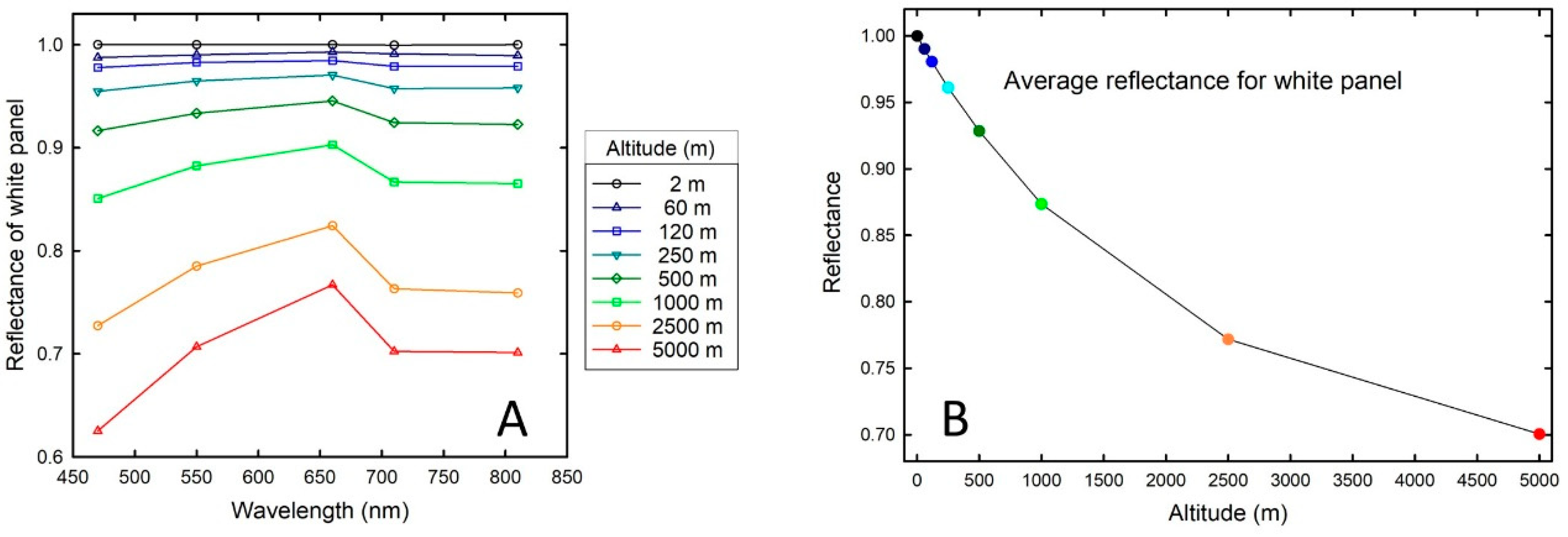
2.3. Effect of Altitude on Retrieved UAS Reflectances

Simulations using the MODTRAN 6 atmospheric radiative transfer model [30] were used to determine the potential magnitude of an altitude effect on Mini-MCA reflectances calculated from an ILS. The atmosphere model is based on mid-latitude summer conditions assuming standard atmospheric pressure and humidity profiles. First, downwelling solar radiance (direct and scattered) was calculated from the top of the atmosphere to the ILS. Second, a white panel (albedo = 100%) at ground level reflected downwelling radiation up to the sensor on the UAS. The ratio of the upwelling spectral radiance from the ground with respect to the downwelling irradiance from the top of the atmosphere was calculated to obtain the apparent spectral reflectance measured at the sensor.
Mini-MCA data from 8 July and 21 July were used to test for an effect of altitude using the ANCOVA test from XLSTAT with the L8-OLI data at a covariate.

3. Results

3.1. Effect of Flight Direction

The stitched orthomosaic reflectance image for 8 July (Figure 3a) from an altitude of 1800 m shows that the southeastern flight lines were much brighter than the northwestern flight lines. Brightness differences between flight lines for the 21 July reflectance image (Figure 3b) were not apparent. In the 8 July image (Figure 3a), the ILS was pointed northwest, away from the sun, during the southeast flight lines, and pointed towards the sun during the northwest flight directions.
Differences in reflectance for the potato fields (Figure 1) were small based on the Landsat data (Figure 2), so the spectral reflectances from the Mini-MCA were compared for these fields (Table 3). On 8 July, reflectances for fields d and f acquired while the aircraft was flying southeast were significantly higher compared to field a, except for the blue band (Table 3). However, on 21 July, the differences between field a and fields d and f were insignificant, except for the 810 nm band. The difference between the two flight directions was just barely significant at an overall level of 0.05 (Table 3).
For Landsat 8 OLI, red reflectances varied between 2% and 20% for the two dates (Figure 4A,C,E), whereas NIR reflectances varied between 20% and 80% (Figure 4B,D,F). These values are consistent with potatoes at peak vegetative growth (red reflectance at 2% and NIR reflectance at 80%) and soils or residue (red and NIR reflectance at about 20%). The relationships between MCA and OLI reflectances were linear, with R2 between 0.719 and 0.936 for the red bands (nine regressions) and 0.819 to 0.913 for the NIR bands (nine regressions). However, all of the slopes between Mini-MCA and OLI were less than 1.0 for a given flight line, showing that the Mini-MCA underestimated reflectances compared to Landsat 8 OLI.
The mean red and NIR reflectances for the southeast flight lines on 8 July were significantly greater (all P < 0.0001) than the red and NIR reflectances determined for the northwest flight lines at all three altitudes (Figure 4). Red reflectances of the southeast flight lines on 21 July were intermediate between the southeast and northwest flight lines on 8 July (Figure 4A,C,E). The 21 July NIR reflectances were significantly lower (all P < 0.0001) than the reflectances from the southeast flight direction on 8 July (Figure 4B,D,F). For the red reflectances, however, the 21 July flight lines were not significantly different from those on 8 July of the southeast flight lines at 650 and 1800 m AGL (Figure 4C,E).

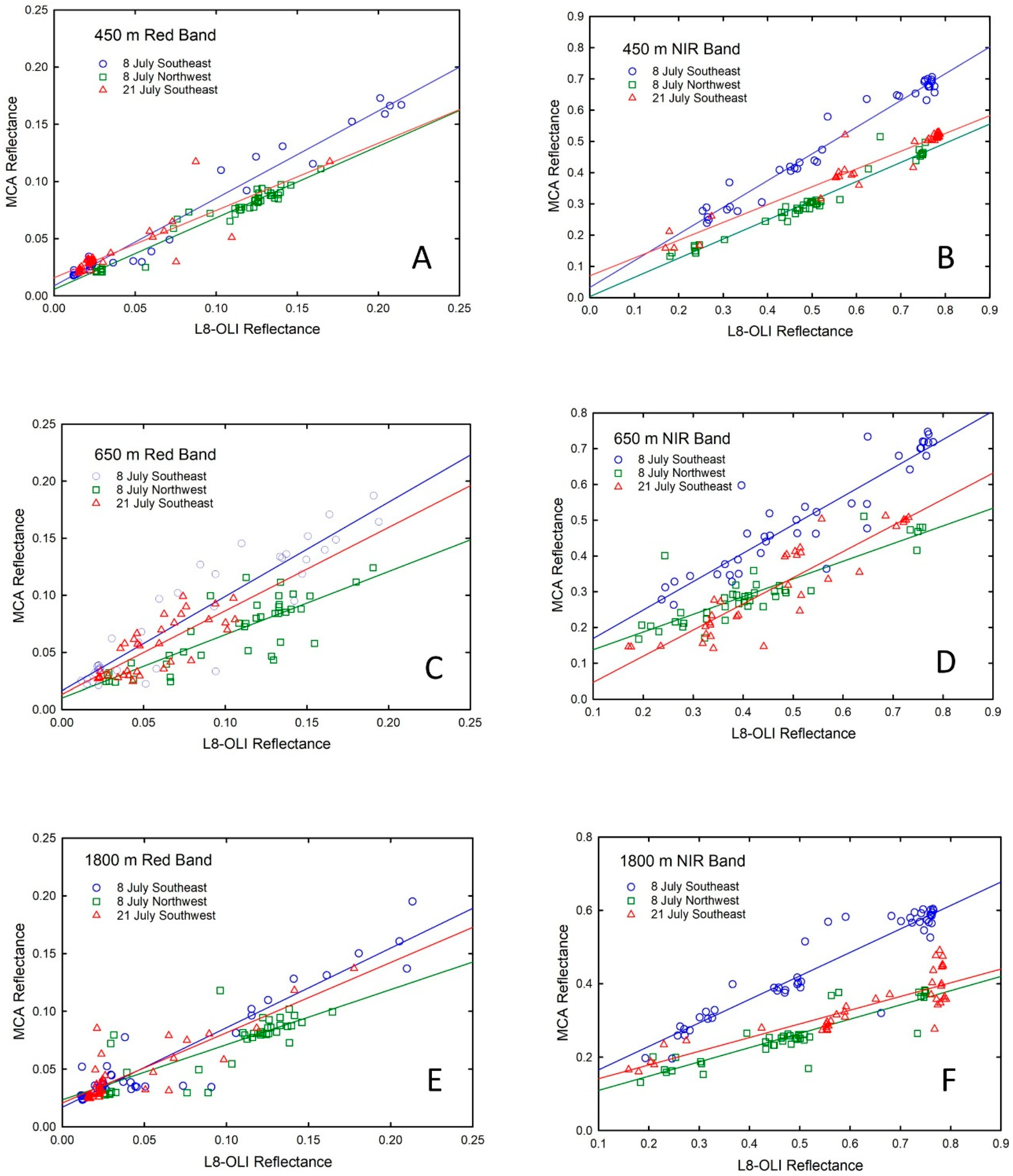
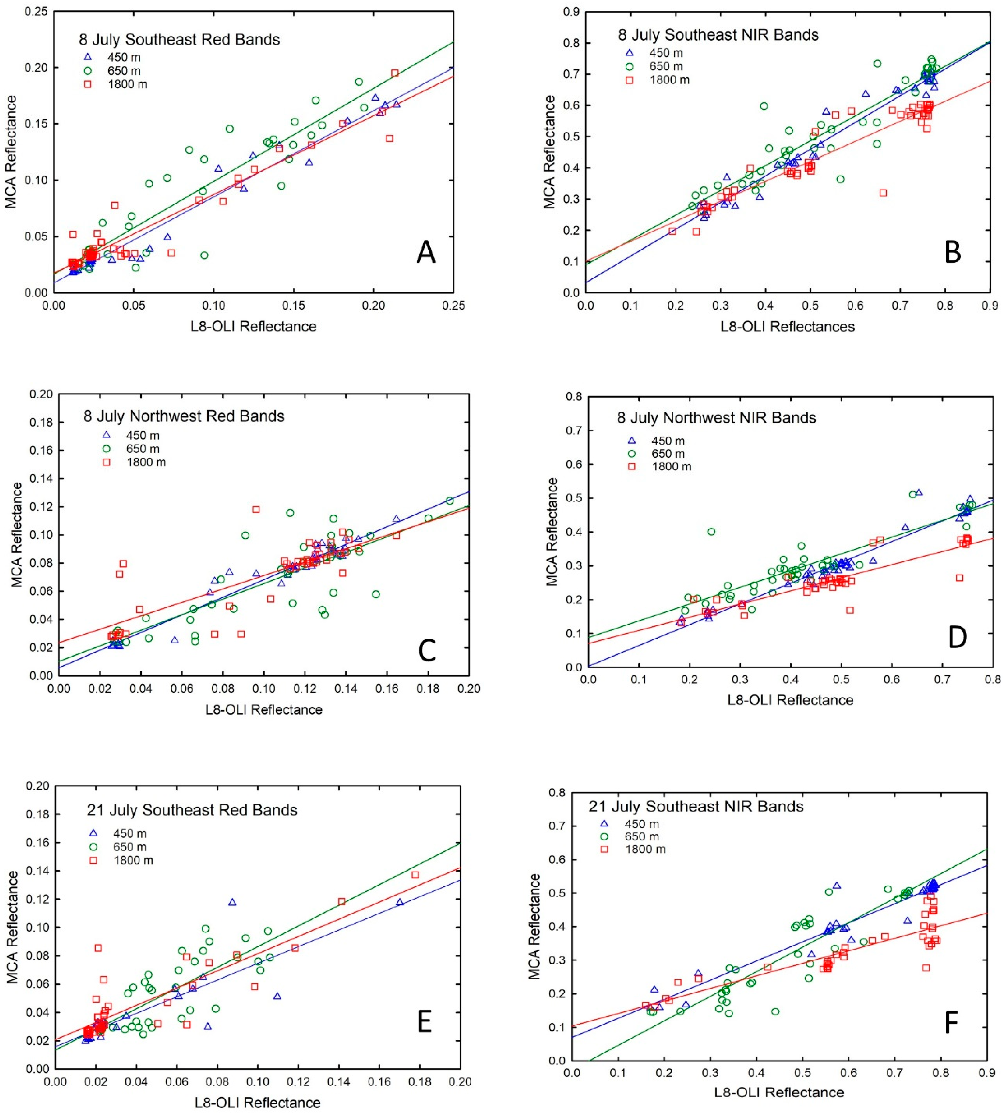
3.2. Effect of Flight Altitude

Simulated reflectances of a white panel on the ground decreased with increasing flight altitude above mean sea level (Figure 5). The larger change at blue wavelengths is the result of Rayleigh scattering, and the larger change at near-infrared wavelengths is the result of atmospheric moisture (Figure 5A). A UAS flying at 120 m above mean sea level would have a 2% decrease in average reflectance compared to reflectances measured on the ground (Figure 5B). Interpolating Figure 5B from 650 m (450 m flight altitude AGL + 200 m ground elevation) to 2000 m (1800 m + 200 m) above mean sea level, reflectance of a white panel would have an 11% decrease from about 90% to about 80%.
To simplify the initial analysis of the effect of altitude, only the flight lines at 450 and 1800 m were compared (Figure 6). The results were consistent. All the comparisons for red bands were not significant with P > 0.05 (Figure 6A,C,E), whereas all the comparisons for the NIR bands were significant at P < 0.0001 (Figure 6B,D,F). The flight lines at the intermediate altitude of 650 m should have reduced red and NIR reflectances compared with flight lines at 450 m. However, the 8 July southeast flight line at 650 m had a significantly greater red reflectance than 450 m at P = 0.001, which is opposite of what was expected (Figure 6A). There were no significant differences (P > 0.05) between the other 450 and 650 m flight lines for both the red and NIR bands (Figure 6B–F). Flight lines with an altitude of 650 m should have greater red and NIR reflectances compared flight lines at 1800 m. All of the NIR comparisons between flight lines at 650 and 1800 m were significant at P < 0.012 or less.

4. Discussion

Up-looking incident light sensors (ILSs) are coupled with down-looking multispectral sensors mounted on UASs to calculate spectral reflectances from the ratio of reflected to incident radiation. The differences in reflectance with aircraft direction on 8 July (Table 3, Figure 4), had to result from changes in the amount of radiation received by either the sensor or ILS. Figure 7 shows the two alternatives.
Irradiance on a surface is equal to the radiant energy of the direct beam times the cosine of the incidence angle (i) between the light source and the normal vector to the surface:
E = cos(i) E0
where E is the irradiance and E0 is the radiant flux density of the direct beam. For solar irradiance on a level ground, the angle of incidence is the solar zenith angle (Figure 7A). The incident light is reflected (or scattered) from a diffuse, Lambertian surface in all directions. A mathematical description of reflected radiant intensity is the BRDF, and the BRDF of a Lambertian surface is a constant. Because there are fewer shadows, plant canopies scatter more light towards the sun (back scatter) than away from the sun (forward scatter). The angle and direction of the maximum radiant intensity is called the hotspot (Figure 7B).
When an aircraft is flying away from the sun, the ILS on the top of the fuselage points toward the sun so the angle of incidence is small (Figure 7C). When the aircraft is flying toward the sun, the ILS points away from the sun so the angle of incidence is large (Figure 7D). The sensor mounted on the bottom of the fuselage points away from the sun, the measured radiation is from canopy back scatter (Figure 7C), and, in the other direction, the sensor measures the canopy forward scatter (Figure 7D).
On 8 July, the solar zenith angle was 38°, and the average pitch angle of the aircraft was 7°; therefore, the ILS angles of incidence are 31° in Figure 7C and 45° in Figure 7D. If there were no change in surface emittance, the retrieved reflectance should be 21% greater when flying the southeast direction, because the emittance is divided by a smaller irradiance. In Table 3, the red reflectance was 27% greater, but the NIR reflectance was 57% greater. If forward and back scatter were significant, then the reflectance in the northwest flight direction would be greater than the reflectance in the southeast flight direction [33]. The center point of the image was adjusted to account for a nadir view angle, but there is no data to confirm if the adjustment was effective. Therefore, it is likely that the difference between the northwest and southeast flight lines on 8 July were caused in part by the direction that the ILS was facing, and not by the BRDF.
The red and NIR reflectances calculated from Mini-MCA bands were less than the reflectances calculated from the L8-OLI red and NIR bands. Without independent data, it is not known whether the calculated Mini-MCA reflectances were underestimated or the calculated L8-OLI reflectances were overestimated. While the focus of the study is on sensor calibration to reflectances, the ILS also needs to be calibrated. Calibration panel images acquired by the Mini-MCA before takeoff and after landing help to adjust the ILS gains to that of the sensor. However, using a calibration panel for adjustment would not have corrected the differences in reflectances caused by flight direction or altitude.
Changes in flight altitude and view angle are usually lessened when using a multirotor UAS compared to a fixed-wing UAS because lift is distributed equally among the rotors. However, the flight duration of multirotor UASs is much less than fixed-wing UASs. A typical flight time with one battery pack for a multirotor UAS carrying a payload is about 20 min. If the air speed is 10 m/s, then the maximum distance for a single battery pack would be about 12 km. The flight lines in this study were about 3 km from start to finish. Without accounting for flight time to achieve the planned altitude and for travel between flight lines, the multirotor UAS could cover the six agricultural fields at 1800 m AGL, but not much more.
Agricultural fields with center pivot irrigation typically are between 25 and 60 ha and may require a faster fixed-wing UAS for full coverage. Non-irrigated fields may be much larger. Flying at higher altitudes is one way to cover more ground in less time. However, altitude becomes another independent factor affecting the calibration of sensor data to reflectance. Furthermore, flying at higher altitudes results in larger ground-sample distances. Hunt and Daughtry [2] argued that one of the important advantages of UAS remote sensing for precision agriculture is the use of small ground-sample distances in order to detect weeds, pest infestations, and diseases. The best altitudes for detection are not known.
There are several options to adjust the ILS readings to calculate irradiance at a given altitude. The first is to measure incident light with ground-based sensors [20]. Since a ground station is employed to control the UAS, incorporating a light sensor with the ground station is practical. This option partially corrects for aircraft altitude; however, the irradiance at a ground station may differ compared to the aircraft because of clouds. More accurate inertial motion units may be used to calculate the incidence angles for an ILS. Finally, there are new ILS designs that can correct for aircraft attitude [21]. Sun photometers are used to determine atmospheric transmittance, which is then used for calculation of solar irradiance. A potential correction for both attitude and altitude is replacing the up-looking sensor with a sun photometer in order to get accurate measurements of atmospheric transmittance [34].
If the sensor/ILS requires radiometric normalization using one calibration panel, why not use the empirical line method to calculate reflectances directly from digital numbers? Instead of one panel, digital numbers are acquired from a UAS-mounted sensor over several calibration targets with a range of measured spectral reflectances [35,36,37,38,39]. The empirical line method is simple and direct, and with small ground sample distances, the targets do not have to be large. For some sensors, at least, there is an interaction between the calibration equation coefficients and shutter speed that is not related to total exposure [40]. Some of the interaction may result from automated camera settings in which the sensor ISO is determined from the shutter speed to avoid image blur. The empirical line method requires constant (or uniformly changing) light conditions, so variation in irradiance during a flight will be missed. Domainzain and Fallet [41] present the calibration equation for a Parrot Sequoia (Paris, France) with an ILS that also corrects for shutter speed, ISO and f-number. They state that the equation is valid if the angle between the sun-target and sensor is taken into consideration [41].
It seems that there are problems inherent in any single method of radiometric calibration of UAS sensors. Therefore, it may be necessary to use a combination of methods to get accurate surface reflectances. These parameters, such as leaf area index and leaf chlorophyll, may be retrieved by either empirical relationships with spectral vegetation indices [6], or by the inversion of canopy radiative transfer models [42,43]. Not all applications using UASs will require this degree of calibration.

5. Conclusions

It is not surprising that UAS flight altitude and attitude affect the apparent surface reflectance values from nadir-looking sensors, and these effects could be predicted based on knowledge from remote sensing with manned aircraft. However, except for a few experiments, ILSs are not deployed on manned aircraft. The justification for having an ILS is that the ratio of up-looking and down-welling radiation is the very definition of reflectance. Therefore, if this method is practical why was it not implemented on manned aircraft? Factors affecting atmospheric transmittance are incorporated into models such as MODTRAN, so it is routine to calculate ground surface reflectances from manned aircraft data. This study suggests that the varying view angles of the ILS created problems for calculating reflectances directly. Sensors for manned aircraft are often mounted on gimbals, so the sensors always have a nadir view. Mounting an ILS on an up-looking gimbal may not be possible. Instead, the orientation of the aircraft with respect to the sun may be calculated with rapid and accurate inertial motion units. To take advantage of these units, not only does the ILS need to be radiometrically calibrated, but the angular responses of the calibration also need to be characterized.

Author Contributions

Conceptualization and methodology, E.R.H.J.; investigation, A.J.S. and E.R.H.J.; writing—original draft and review & editing, E.R.H.J.; visualization, A.J.S.; supervision and project administration, E.R.H.J.

Funding

This research received no external funding.

Acknowledgments

We thank Dan Fuller for planning the flights and piloting the UAS. Also, we thank the three reviewers for their efforts improving the manuscript.

Conflicts of Interest

The authors declare no conflict of interest.

Notice

USDA is an equal opportunity employer and provider.

Disclaimer

Mention of commercial names in this paper does not constitute an endorsement by the authors, the Agricultural Research Service, or the United States Department of Agriculture.

References

  1. Zhang, C.; Kovacs, J.M. The application of small unmanned aerial systems for precision agriculture: A review. Precis. Agric. 2012, 13, 693–712. [Google Scholar] [CrossRef]
  2. Hunt, E.R.J.; Daughtry, C.S. What good are unmanned aircraft systems for agricultural remote sensing and precision agriculture? Int. J. Remote Sens. 2018, 39, 5345–5376. [Google Scholar] [CrossRef]
  3. Barbedo, J.G.A. A Review on the Use of Unmanned Aerial Vehicles and Imaging Sensors for Monitoring and Assessing Plant Stresses. Drones 2019, 3, 40. [Google Scholar] [CrossRef]
  4. Maes, W.H.; Steppe, K. Perspectives for remote sensing with unmanned aerial vehicles in precision agriculture. Trends Plant. Sci. 2019, 24, 152–164. [Google Scholar] [CrossRef]
  5. Franceschini, M.H.; Bartholomeus, H.; Van Apeldoorn, D.F.; Suomalainen, J.; Kooistra, L. Feasibility of unmanned aerial vehicle optical imagery for early detection and severity assessment of late blight in potato. Remote Sens. 2019, 11, 224. [Google Scholar] [CrossRef]
  6. Daughtry, C.S.; Walthall, C.L.; Kim, M.S.; De Colstoun, E.B.; McMurtrey, J.E., III. Estimating corn leaf chlorophyll concentration from leaf and canopy reflectance. Remote Sens. Environ. 2000, 74, 229–239. [Google Scholar] [CrossRef]
  7. Zheng, H.; Li, W.; Jiang, J.; Liu, Y.; Cheng, T.; Tian, Y.; Zhu, Y.; Cao, W.; Zhang, Y.; Yao, X. A comparative assessment of different modeling algorithms for estimating leaf nitrogen content in winter wheat using multispectral images from an unmanned aerial vehicle. Remote Sens. 2018, 10, 2026. [Google Scholar] [CrossRef]
  8. Hunt, E.R.; Hively, W.D.; Fujikawa, S.; Linden, D.; Daughtry, C.S.; McCarty, G. Acquisition of NIR-green-blue digital photographs from unmanned aircraft for crop monitoring. Remote Sens. 2010, 2, 290–305. [Google Scholar] [CrossRef]
  9. Kelcey, J.; Lucieer, A. Sensor correction of a 6-band multispectral imaging sensor for UAV remote sensing. Remote Sens. 2012, 4, 1462–1493. [Google Scholar] [CrossRef]
  10. Mamaghani, B.G.; Sasaki, G.V.; Connal, R.J.; Kha, K.; Knappen, J.S.; Hartzell, R.A.; Marcellus, E.D.; Bauch, T.D.; Raqueño, N.G.; Salvaggio, C. An initial exploration of vicarious and in-scene calibration techniques for small unmanned aircraft systems. In Autonomous Air and Ground Sensing Systems for Agricultural Optimization and Phenotyping III; Thomasson, J.A., McKee, M., Moorhead, R.J., Eds.; International Society for Optics and Photonics: Bellingham, WA, USA, 2018. [Google Scholar] [CrossRef]
  11. Cao, S.; Danielson, B.; Clare, S.; Koenig, S.; Campos-Vargas, C.; Sanchez-Azofeifa, A. Radiometric calibration assessments for UAS-borne multispectral cameras: Laboratory and field protocols. ISPRS J. Photogram. Remote Sens. 2019, 149, 132–145. [Google Scholar] [CrossRef]
  12. Edwards, J.; Anderson, J.; Shuart, W.; Woolard, J. An evaluation of reflectance calibration methods for UAV spectral imagery. Photogram. Eng. Remote Sens. 2019, 85, 221–230. [Google Scholar] [CrossRef]
  13. Jiang, J.; Zheng, H.; Ji, X.; Cheng, T.; Tian, Y.; Zhu, Y.; Cao, W.; Ehsani, R.; Yao, X. Analysis and evaluation of the image preprocessing process of a six-band multispectral camera mounted on an unmanned aerial vehicle for winter wheat monitoring. Sensors 2019, 19, 747. [Google Scholar] [CrossRef] [PubMed]
  14. Roosjen, P.; Suomalainen, J.; Bartholomeus, H.; Kooistra, L.; Clevers, J. Mapping reflectance anisotropy of a potato canopy using aerial images acquired with an unmanned aerial vehicle. Remote Sens. 2017, 9, 417. [Google Scholar] [CrossRef]
  15. Aasen, H.; Honkavaara, E.; Lucieer, A.; Zarco-Tejada, P. Quantitative remote sensing at ultra-high resolution with UAV spectroscopy: A review of sensor technology, measurement procedures, and data correction workflows. Remote Sens. 2018, 10, 1091. [Google Scholar] [CrossRef]
  16. Honkavaara, E.; Khoramshahi, E. Radiometric correction of close-range spectral image blocks captured using an unmanned aerial vehicle with a radiometric block adjustment. Remote Sens. 2018, 10, 256. [Google Scholar] [CrossRef]
  17. Tu, Y.H.; Phinn, S.; Johansen, K.; Robson, A. Assessing radiometric correction approaches for multi-spectral UAS imagery for horticultural applications. Remote Sens. 2018, 10, 1684. [Google Scholar] [CrossRef]
  18. Stow, D.; Nichol, C.J.; Wade, T.; Assmann, J.J.; Simpson, G.; Helfter, C. Illumination geometry and flying height influence surface reflectance and NDVI derived from multispectral UAS imagery. Drones 2019, 3, 55. [Google Scholar] [CrossRef]
  19. Hakala, T.; Honkavaara, E.; Saari, H.; Mäkynen, J.; Kaivosoja, J.; Pesonen, L.; Pölönen, I. Spectral imaging from UAVs under varying illumination conditions. Int. Arch. Photogramm. Remote Sens. Spatial Infor. Sci. 2013, XL-1/W2, 189–194. [Google Scholar] [CrossRef]
  20. Hakala, T.; Markelin, L.; Honkavaara, E.; Scott, B.; Theocharous, T.; Nevalainen, O.; Näsi, R.; Suomalainen, J.; Viljanen, N.; Greenwell, C.; et al. Direct reflectance measurements from drones: Sensor absolute radiometric calibration and system tests for forest reflectance characterization. Sensors 2018, 18, 1417. [Google Scholar] [CrossRef]
  21. Suomalainen, J.; Hakala, T.; Alves de Oliveira, R.; Markelin, L.; Viljanen, N.; Näsi, R.; Honkavaara, E. A novel tilt correction technique for irradiance sensors and spectrometers on-board unmanned aerial vehicles. Remote Sens. 2018, 10, 2068. [Google Scholar] [CrossRef]
  22. Yu, X.; Liu, Q.; Liu, X.; Liu, X.Y.; Wang, Y. A physical-based atmospheric correction algorithm of unmanned aerial vehicles images and its utility analysis. Int. J. Remote Sens. 2017, 38, 3101–3112. [Google Scholar] [CrossRef]
  23. FAA. Integration of Civil Unmanned Aircraft Systems (UAS) in the National Airspace System (NAS) Roadmap, 2nd ed.; Federal Aviation Administration: Washington, DC, USA, 2018. Available online: https://www.faa.gov/uas/resources/policy_library/second_edition_integration_of_civil_UAS_NAS_roadmap_July 2018.pdf (accessed on 27 September 2019).
  24. Watts, A.C.; Ambrosia, V.G.; Hinkley, E.A. Unmanned aircraft systems in remote sensing and scientific research: Classification and considerations of use. Remote Sens. 2012, 4, 1671–1692. [Google Scholar] [CrossRef]
  25. Boryan, C.; Yang, Z.; Mueller, R.; Craig, M. Monitoring US agriculture: The US Department of Agriculture, National Agricultural Statistics Service, Cropland Data Layer Program. Geocarto Int. 2011, 26, 341–358. [Google Scholar] [CrossRef]
  26. Heinold, S. Radiometric Multi-Spectral or Hyperspectral Camera Array Using Matched Area Sensors and a Calibrated Ambient Light Collection Device. U.S. Patent 2014 0022381 A1, 23 January 2014. [Google Scholar]
  27. Vermote, E.; Justice, C.; Claverie, M.; Franch, B. Preliminary analysis of the performance of the Landsat 8/OLI land surface reflectance product. Remote Sens. Environ. 2016, 185, 46–56. [Google Scholar] [CrossRef]
  28. Markham, B.; Barsi, J.; Kvaran, G.; Ong, L.; Kaita, E.; Biggar, S.; Czapla-Myers, J.; Mishra, N.; Helder, D. Landsat-8 operational land imager radiometric calibration and stability. Remote Sens. 2014, 6, 12275–12308. [Google Scholar] [CrossRef]
  29. Czapla-Myers, J.; McCorkel, J.; Anderson, N.; Thome, K.; Biggar, S.; Helder, D.; Aaron, D.; Leigh, L.; Mishra, N. The ground-based absolute radiometric calibration of Landsat 8 OLI. Remote Sens. 2015, 7, 600–626. [Google Scholar] [CrossRef]
  30. Berk, A.; Conforti, P.; Kennett, R.; Perkins, T.; Hawes, F.; van den Bosch, J. MODTRAN© 6: A major upgrade of the MODTRAN radiative transfer code. In Algorithms and Technologies for Multispectral, Hyperspectral, and Ultraspectral Imagery XX, Proceedings of the SPIE 9088, Bellingham, WA, USA, 23–27 February 2014; Velez-Reyes, M., Kruse, F.A., Eds.; International Society for Optics and Photonics: Bellingham, WA, USA, 2014; p. 90880H. [Google Scholar] [CrossRef]
  31. Adler-Golden, S.M.; Matthew, M.W.; Bernstein, L.S.; Levine, R.Y.; Berk, A.; Richtsmeier, S.C.; Acharya, P.K.; Anderson, G.P.; Felde, G.; Gardner, J.; et al. Atmospheric Correction for Short-wave Spectral Imagery Based on MODTRAN4. In Imaging Spectrometry V, Proceedings of the SPIE 3753; Descour, M.R., Shen, S.S., Eds.; International Society for Optics and Photonics: Bellingham, WA, USA, 1999; pp. 61–69. [Google Scholar] [CrossRef]
  32. Hill, T.; Lewicki, P. Statistics Methods and Applications; StatSoft: Tulsa, OK, USA, 2006; pp. 48–49. [Google Scholar]
  33. Zhao, F.; Li, Y.; Dai, X.; Verhoef, W.; Guo, Y.; Shang, H.; Gu, X.; Huang, Y.; Yu, T.; Huang, J. Simulated impact of sensor field of view and distance on field measurements of bidirectional reflectance factors for row crops. Remote Sens. Environ. 2015, 156, 129–142. [Google Scholar] [CrossRef]
  34. Walthall, C.L.; Halthore, R.N.; Loechel, S.E.; Elman, G.C.; Markham, B.L. Measuring aerosol optical thickness with a helicopter-based sunphotometer. IEEE Ts. Geosci. Remote Sens. 2000, 38, 1410–1416. [Google Scholar] [CrossRef]
  35. Roberts, D.A.; Yamaguchi, Y.; Lyon, R.J.P. Comparison of various techniques for calibration of AIS data. In JPL Proceedings of Second Airborne Imaging Spectrometer Data Analysis Workshop; Vane, G., Goetz, A.F.H., Eds.; Jet Propulsion Laboratory: Pasadena, CA, USA, 1986; JPL publication 86–35; pp. 21–30. [Google Scholar]
  36. Smith, G.M.; Milton, E.J. The use of the empirical line method to calibrate remotely sensed data to reflectance. Int. J. Remote Sens. 1999, 20, 2653–2662. [Google Scholar] [CrossRef]
  37. Hunt, E.R., Jr.; Cavigelli, M.; Daughtry, C.S.T.; McMurtrey, J., III; Walthall, C.L. Evaluation of digital photography from model aircraft for remote sensing of crop biomass and nitrogen status. Precis. Agric. 2005, 6, 359–378. [Google Scholar] [CrossRef]
  38. Baugh, W.M.; Groeneveld, D.P. Empirical proof of the empirical line. Int. J. Remote Sens. 2008, 29, 665–672. [Google Scholar] [CrossRef]
  39. Wang, C.; Myint, S.W. A simplified empirical line method of radiometric calibration for small unmanned aircraft systems-based remote sensing. IEEE J. Sel. Top. Appl. 2015, 8, 1876–1885. [Google Scholar] [CrossRef]
  40. Hunt, E.R., Jr.; Horneck, D.A.; Spinelli, C.B.; Turner, R.W.; Bruce, A.E.; Gadler, D.J.; Brungardt, J.J.; Hamm, P.B. Monitoring nitrogen status of potatoes using small unmanned aerial vehicles. Precis. Agric. 2018, 19, 314–333. [Google Scholar] [CrossRef]
  41. Domenzain, L.M.; Fallet, C. Necessary steps for the systematic calibration of a multispectral imaging system to achieve a targetless workflow in reflectance estimation: A study of Parrot SEQUOIA for precision agriculture. In Algorithms and Technologies for Multispectral, Hyperspectral, and Ultraspectral Imagery XXIV, Proceedings of the SPIE 10644, San Jose, CA, USA, 25 February–1 March 2018; Velez-Reyes, M., Messinger, D.W., Eds.; International Society for Optics and Photonics: Bellingham, WA, USA, 2018; Volume 1064416. [Google Scholar] [CrossRef]
  42. Jacquemoud, S.; Verhoef, W.; Baret, F.; Bacour, C.; Zarco-Tejada, P.J.; Asner, G.P.; François, C.; Ustin, S.L. PROSPECT+ SAIL models: A review of use for vegetation characterization. Remote Sens. Environ. 2009, 113, S56–S66. [Google Scholar] [CrossRef]
  43. Duan, S.B.; Li, Z.L.; Wu, H.; Tang, B.H.; Ma, L.; Zhao, E.; Li, C. Inversion of the PROSAIL model to estimate leaf area index of maize, potato, and sunflower fields from unmanned aerial vehicle hyperspectral data. Int. J. Appl. Earth Obs. 2014, 26, 12–20. [Google Scholar] [CrossRef]
Figure 1. Experimental layout for Unmanned Aircraft Systems (UAS) flights on two dates over six agricultural fields with center-pivot irrigation and two fields of sagebrush steppe. Fields (a), (c), (e), and (g) were always flown with a northwest bearing, whereas fields (b), (d), (f), and (h) were always flown with a southeast bearing. Flight lines were 29° from alignment with the solar azimuth on 8 July 2014, whereas the flight lines were 6° from being perpendicular to the solar azimuth on 21 July 2014. Each flight consisted of three altitudes: 650, 450, and 1800 m above ground level (AGL). Colors represent potato (light green; fields a, d, and f), spring wheat (tan; fields c and e), maize (yellow; field b), and sagebrush steppe (brown; fields g and h).
Remotesensing 11 02622 g001
Figure 2. Color-infrared false-color composite of Landsat 8 OLI (path 044, row 028) reflectances acquired on (A) 8 July 2014 and (B) 24 July 2014. Because of the clouds and shadows in (B), only the southeast flight line was used for each aircraft altitude.
Remotesensing 11 02622 g002
Figure 3. (A) Color-infrared orthomosaic image from the 8 July 2014 UAS flight at 1800 m AGL. (B) Color-infrared orthomosaic image from the 21 July 2014 UAS flight at 1800 m AGL. Crop type and UAS flight directions are shown in Figure 1.
Remotesensing 11 02622 g003
Figure 4. Comparison of Mini-MCA and Landsat 8 OLI reflectances acquired from southeast and northwest flight directions at three altitudes AGL on 8 July and 21 July 2014: (A) red reflectance at 450 m, (B) NIR reflectance at 450 m, (C) red reflectance at 650 m, (D) NIR reflectance at 650 m, (E) red reflectance at 1800 m, and (F) NIR reflectance at 1800 m.
Remotesensing 11 02622 g004
Figure 5. (A) Simulated spectra of a white panel on the ground with a sensor/ILS at various altitudes above mean sea level using the MODTRAN 6 model. (B) Average reflectance of the white panel from the sensor/ILS at various altitudes.
Remotesensing 11 02622 g005
Figure 6. Comparison of three flight altitudes AGL for: 8 July southeast flight lines (A) red bands and (B) NIR bands; 8 July northwest flight lines (C) red bands and (D) NIR bands; and 21 July southeast flight lines (E) red bands and (F) NIR bands.
Remotesensing 11 02622 g006
Figure 7. Bidirectional Reflectance Distribution Functions (BRDF) for (A) a Lambertian surface and (B) a plant canopy. Effect of plane attitude on an up-looking ILS when (C) flying away from the sun and (D) flying towards the sun. The red lines in (A) and (B) are pointing perpendicular to level ground and defining the nadir direction. The zenith angle is the direction between the nadir and the sun’s position and is the solar incidence angle on a level surface. The two red lines in (C) and (D) are perpendicular to the top surface of the aircraft and nadir view for a sensor. (C) shows the orientation for northwest flights on 8 July and (D) shows the orientation for southeast flights.
Remotesensing 11 02622 g007
Table 1. Minimum and maximum wavelengths (nm) for bands of the Tetracam, Inc. Miniature Multiple Camera Array (Mini-MCA) and Landsat 8 Operational Line Imager (L8-OLI).
BandMini-MCALandsat 8 OLI
Blue460–480450–510
Green540–560530–590
Red650–670640–670
Red-edge700–720not present
Near-infrared (NIR)800–820850–880
Table 2. Coverage of the Mini-MCA at three altitudes above ground level.
Altitude (m)Ground Sample Distance (mm)Field of View (ha)Number of Flight LinesFront-to-Back Overlap (%)Side-to-Side Overlap (%)
4502447.81677.823.8
65035216.21084.425.7
1800975125294.834.2
Table 3. Comparison of Mini-MCA reflectances of potato fields on two dates. Field labels are shown in Figure 1. Rmean and RSD are reflectance (dimensionless) mean and standard deviation, respectively; P is the probability* that the null hypothesis was correct.
WavelengthField aFields d & fP
RmeanRSDRmeanRSD
8 July 20144700.03850.00270.04220.00400.1335
5500.07210.00330.08310.00430.0021
6600.02970.00260.03790.00380.0059
7100.13670.00530.18110.0085<0.0001
8100.36940.01470.57840.0355<0.0001
21 July 20144700.03820.00300.04140.00440.1894
5500.06980.00330.06930.00770.4681
6600.03390.00380.03870.00550.1587
7100.16020.00650.14430.01560.0918
8100.43190.01880.37150.03620.0183
* The level for significance of the Z test is P < 0.025 for an overall level of significance of 0.05, because the hypothesis required a two-tailed test.

