Abstract
Management and control operations are crucial for preventing forest fires, especially in Mediterranean forest areas with dry climatic periods. One of them is prescribed fires, in which the biomass fuel present in the controlled plot area must be accurately estimated. The most used methods for estimating biomass are time-consuming and demand too much manpower. Unmanned aerial vehicles (UAVs) carrying multispectral sensors can be used to carry out accurate indirect measurements of terrain and vegetation morphology and their radiometric characteristics. Based on the UAV-photogrammetric project products, four estimators of phytovolume were compared in a Mediterranean forest area, all obtained using the difference between a digital surface model (DSM) and a digital terrain model (DTM). The DSM was derived from a UAV-photogrammetric project based on the structure from a motion algorithm. Four different methods for obtaining a DTM were used based on an unclassified dense point cloud produced through a UAV-photogrammetric project (FFU), an unsupervised classified dense point cloud (FFC), a multispectral vegetation index (FMI), and a cloth simulation filter (FCS). Qualitative and quantitative comparisons determined the ability of the phytovolume estimators for vegetation detection and occupied volume. The results show that there are no significant differences in surface vegetation detection between all the pairwise possible comparisons of the four estimators at a 95% confidence level, but FMI presented the best kappa value (0.678) in an error matrix analysis with reference data obtained from photointerpretation and supervised classification. Concerning the accuracy of phytovolume estimation, only FFU and FFC presented differences higher than two standard deviations in a pairwise comparison, and FMI presented the best RMSE (12.3 m) when the estimators were compared to 768 observed data points grouped in four 500 m2 sample plots. The FMI was the best phytovolume estimator of the four compared for low vegetation height in a Mediterranean forest. The use of FMI based on UAV data provides accurate phytovolume estimations that can be applied on several environment management activities, including wildfire prevention. Multitemporal phytovolume estimations based on FMI could help to model the forest resources evolution in a very realistic way.
1. Introduction
Controlling and managing above-ground vegetation has crucial importance in studies related to reducing carbon emissions [1] or associated with deforestation and forest degradation [2]. Both effects are increased by wildland fires and progressive abandonment of farming lands [3,4]. Biomass is a key structural variable in all the studies about ecosystem dynamics, biodiversity, and sustainability [3,5,6]. For example, maps of forest fuel were obtained by [7], and the spatiotemporal evolution of the risk of forest fire using landsat satellite imagery was studied by [8]. The dynamics of the biomass structure were analysed by [9] and related to different stages of flammability.
According to [4,10], the importance of shrublands in the Mediterranean ecosystem is very high due to their significance in the forest dynamic and the large swathe of territory occupied, but most of the studies carried out in the literature are about the biomass of tree species [11,12,13]. Biomass estimation in a forest environment can be undertaken in a direct way by harvesting and weighing sampled plant material [14] or indirectly by measuring morphological variables and applying mathematical models. The first method generates more accurate estimations but is more time-consuming, while the second is indicated for multitemporal studies. A mixed model consists of harvesting a sample of plant material and calibrating the mathematical model using the collected data [4,9].
Phytovolume is the volume under vegetal canopy, while biomass represents the weight of the aerial part of the vegetation. The relationship between biomass and phytovolume using apparent density was applied by [15] for indirect estimation of biomass, demonstrating that phytovolume is a good estimator of biomass with regression coefficients of up to 90%. Species were characterised by their apparent density and biomass ratio, which were modelled through regressions between phytovolume and biomass. In another study, model regressions were characterised between biomass and phytovolume for 16 Mediterranean shrub species divided into five density classes [16]. Phytovolume was used by [17] for demonstrating significant differences between two management systems, grazing and not-grazing, with respect to the flammability of forest resources.
Instead of harvested plant material, aerial data have been widely used for indirect measurement in the literature, including optical, SAR, LiDAR, and unmanned aerial vehicle (UAV) data-based methods with the empirical radiative transfer model, machine learning algorithms, and artificial intelligence.
Artificial neural network (ANN) models incorporating radar data performed better in estimating phytomass than ANN models, using only optical vegetation indices with r-squared values of 0.79 and 0.6, respectively [18]. Other studies centred on multispectral satellite imagery were carried out by [19], who used height and diameter data and a classification of cover fraction based on Quickbird and Landsat imagery for mapping fuel type. A comparison of eight spectral indices of vegetation based on MODIS imagery for fire prediction purposes was undertaken by [20].
LiDAR point cloud information and multispectral imagery were combined to obtain fuel maps with up to 85.43% global agreement, using object-based image analysis (OBIA) [7]. The height of the canopy was measured with LiDAR and hyperspectral sensors by [15] for adjusting regressions to biomass. The same source of data was used by [6] for obtaining biomass and stress maps. A complete review of the accuracies obtained in biomass estimations based on LiDAR data by different authors can be read in [3].
Biomass was monitored by [21] using P-band SAR with multitemporal observations, concluding that P-bands are the most suited frequency for above-ground biomass of boreal forests; multitemporal satellite imagery and SAR data were combined by [22] for above-ground biomass estimation reaching an adjusted R2 of 0.43 and RMSE of around 70 Mg/ha; and above-ground biomass was estimated by [23,24] from UAV data at a different scale levels, obtaining correlations of r2 = 0.67, RMSE = 344 g/m2 and r2 = 0.98, RMSE = 91.48 g/m2, respectively.
Phytovolume can be obtained by taking the difference between the digital surface model (DSM), which involves the canopy and base soil between vegetation clusters, and the digital terrain model (DTM), which covers the terrain surface without vegetation [25].
The Mediterranean shrubland has low-lying vegetation with a relatively high fractional vegetation cover (FVC) [5,17]. These characteristics compromise the phytovolume modelling for two main reasons: The point clouds obtained from photogrammetric methods, radar, or LiDAR, have a low density of points located at the bare soil, and the radiometric methods based on multispectral imagery classification tend to underestimate the phytovolume due to the difficulty of dead vegetation detection.
With the recent development of civilian use of UAVs, a large variety of sensors with the capacity for close-range sensing has been applied in environmental engineering in general and for monitoring specific ecosystem variables [26,27,28]. Digital cameras operating in the visible spectrum are used for UAV-photogrammetric projects combined with the structure from motion (SfM) [29] and multi-view stereopsis (MVS) [30] techniques, producing very high-resolution orthoimages, DSMs, DTMs, and very dense point clouds of the terrain [31,32]. Most of the indices designed for remote sensing based on satellite imagery can be applied or adapted to multispectral sensors mounted on UAVs.
Due to the low altitude of flights and the high resolution of the sensors carried by UAVs, the accuracies of photogrammetric products can reach 0.053 m, 0.070 m, and 0.061 m in the X, Y, and Z directions, respectively, even in environs with extreme topography [33]. These accuracy levels make it possible to evaluate phytovolume at a local scale and to calibrate satellite data based on a regional scale. In this way, biomass estimation becomes more efficient, even in inaccessible mountain areas.
Furthermore, the spatiotemporal monitoring of phytovolume can be undertaken when UAVs operate in autonomous navigation mode with programmed flight routes, thanks to the control devices based on the global navigation satellite system (GNSS). Unlike in satellite imagery, the temporal resolution of UAV imagery is controlled by the user, so flights can be programmed to register a dramatic change of phytovolume, e.g., pre- and post-fire [27].
This work aimed to evaluate the ability of four phytovolume estimation methods, all obtained using the difference between DSM and DTM, based on very high-resolution spatial imagery collected by a multispectral sensor onboard a UAV. If phytovolume could be accurately estimated based on UAV-photogrammetry and multispectral imagery, then a new indirect method for indirect biomass estimation could be developed, characterising the apparent density of the predominant vegetation.
The DSM was obtained from the UAV-photogrammetric process, while the four DTMs were calculated following the most common methods in bibliography about multispectral imagery, that is, interpolation of unclassified dense point cloud produced through a UAV-photogrammetric project and interpolation of unsupervised classified dense point cloud based on a multispectral vegetation index and using a cloth simulation filter.
2. Materials and Methods
In the four methods compared in this paper, the DSM was derived from a UAV-photogrammetric project based on the SfM algorithm, and the four DTMs were based on the unclassified dense point cloud produced by a UAV-photogrammetric project (FFU), an unsupervised classified dense point cloud (FFC) [34], a multispectral vegetation index (FMI), and a cloth simulation filter (FCS) [35].
The input data for obtaining the four phytovolume maps included multispectral imagery with visible red edge, and near-infrared bands obtained from a UAV-photogrammetric flight and in situ sample data collected at the same time as the UAV flight. The flight was carried out in a Mediterranean shrubland located on the northern face of the Sierra de los Filabres, belonging to the siliceous territory of the Nevado–Filábride complex in the Almeria province of southern Spain.
The differences between the DTM obtained from the UAV-photogrammetric project and the four DTMs obtained from different criteria were expressed in terms of phytovolume maps and compared to find statistical differences between them. Qualitative and quantitative comparisons determined the ability of the four models to detect vegetation and to measure the apparent volume occupied by the vegetation groups. The corresponding four comparisons with in situ sample data determined the best estimator of phytovolume.
2.1. Study Area
The experimental plot was located on the northern face of the Sierra de los Filabres with geographic coordinates 37°18’35.30″N, 2°36’9.67″W (European Terrestrial Reference System 1989, ETRS89) (Figure 1) in the Alcóntar municipality in the province of Almería (Spain), belonging to the Béticas mountain range [36]. The forest is 5.5 km and 3.5 km from the Special Areas of Conservation of Calares de Sierra de Baza and Sierra de Baza, respectively, which are included in the European Natura 2000 Protected Areas Network [37].
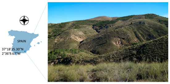
Figure 1.
Location and landscape of the study area in Sierra de los Filabres, Almería province, southern Spain.
The climate in Sierra de los Filabres is classified as semi-arid Mediterranean with a short, warm, arid summer and a long, cold, dry winter. The annual average temperature is 13.9 °C, and the annual average precipitation is 444 mm. Precipitation is scarce and irregular, and pluriannual droughts are relatively frequent and intense.
The potential vegetation includes mid-mountain basophil holm oaks. Shrubs in regressive phase abound due to anthropogenic action on the territory, which is now abandoned, including old rain-fed crops, mining, and recent reforestation. The two most frequent species are gorse (Genista scorpius) and esparto grass (Macrochloa tenacissima), although some others appear in minor proportion, like Bupleurum falcatum, Helianthemum nummularium, Astragalus propinquus, and Retama sphaerocarpa L.
According to the Environmental Information Network of Andalusia (REDIAM) [33], soils in the study area are classified as eutric cambisols, eutric regosols, and chromic luvisols with lithosols.
The total surface of the study area was 3.41 ha with an average elevation of 1288.46 m above sea level, ranging from 1233 m to 1240 m, and the average slope was 41.51%.
2.2. Unmanned Aerial Vehicle and Sensor
The UAV-photogrammetric flight was carried out on 17 December 2018, on a sunny day (Figure 2).
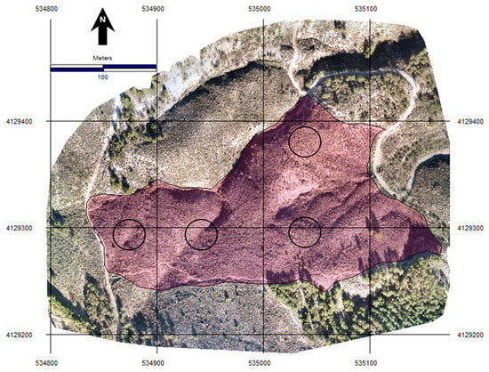
Figure 2.
Orthophoto of the study area. The predominant species are Genista scorpius and Macrochloa tenacissima. Circles represent the four parcels with a surface of 500 m2 distributed throughout the study area to characterise the species distribution.
The UAV used in this work was equipped with a Parrot Sequoia multispectral camera [38] mounted on a motion-compensated three-axis gimbal, and the chosen platform was a rotatory wing DJI Matrice 600 Pro UAV with six rotors (Figure 3).
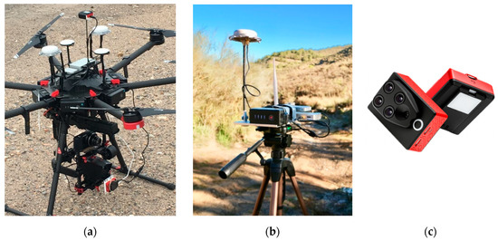
Figure 3.
Unmanned Aerial Vehicle (UAV) system: (a) DJI Matrice 600 Pro with a Parrot Sequoia multispectral camera onboard and D-RTK navigation antennas; (b) base station of the D-RTK Global Navigation Satellite System (GNSS) positioning and navigation device; (c) multi-spectral Sequoia cam with a sunshine sensor.
The Parrot Sequoia camera collects multispectral imagery that includes the green, red, red-edge, and near-infrared wavelengths through four 1.2-megapixel (1280 × 960) sensors (Figure 3). The focal length of the four lenses is fixed at 4 mm, and horizontal and vertical FOVs of 61.9 and 48.5, respectively. When the flight height above ground level is 56 m, the average ground sample distance (GSD) is 3 cm. The camera also collects Red, Green and Blue (RGB) imagery with an integrated high-resolution 16-megapixel (4608 × 3456) sensor that reaches a 1.5 cm GSD at a 56 m flight height.
Light conditions in the same spectral bands as the multispectral sensor are captured by an irradiance sensor to collect irradiance during flight operations and correct possible fluctuations, calculating the absolute reflectance in post-processing.
UAV positioning is based on a differential real-time kinematic (d-RTK) device composed of a double antenna onboard the UAV, a base station that emits real-time corrections from land, and a GNSS triple-redundant antenna system. The horizontal and vertical positioning accuracies that can be achieved are 1 cm + 1 ppm and 2 cm + 1 ppm, respectively, and 1.3 degrees in orientation.
2.3. Flight Route Planning
Scale heterogeneity is one of the most important problems to solve in photogrammetry, especially when the flight altitude is low and the terrain to model is steep. In UAV-photogrammetry, the flight routes can be planned to maintain a constant distance over the terrain.
In this work, UgCS 3.0 PRO software [39] was applied for designing a flight route with a constant 56.2 m altitude above ground level (AGL) (Figure 4), based on a prospective low-resolution DSM previously processed with a UAV general flight.
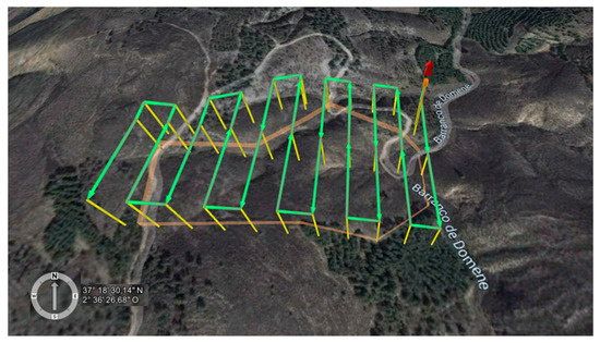
Figure 4.
Flight planning with waypoints at the same 56.2 m altitude above ground level (AGL).
A total of 1220 visible and multispectral images were acquired during the flight carried out with longitudinal and transversal overlaps of 70% and 55%, respectively, and a 23 min total flight time at 4 m/s. At the time of flights, the sun elevation ranged from 23.71° to 29.33°.
2.4. Survey Campaign
All the products obtained from the photogrammetric project, including DSM, DTM, and point cloud, must be referenced to the same coordinate system to be processed. The imagery co-registration and georeferencing was undertaken based on the ETRS89 coordinates of ten ground control points (GCPs) that were scattered on the study area following the recommendations of [32,40]. The three-dimensional (3D) coordinates of GCPs were measured with a very accurate device composed of a receptor Trimble R6 working in the post-processed kinematic (PPK) mode and a wayside base station (Figure 5).
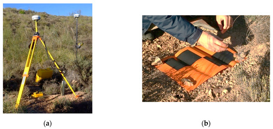
Figure 5.
Surveying campaign: (a) Trimble R6 Rover and base GNSS receivers; (b) target for the ground control points (GCPs).
The post-processing of the measured coordinates of GCPs was undertaken by Trimble Real-Time eXtended (RTX) correction services [41]. This high-accuracy global GNSS technology combines real-time data with positioning and compression algorithms that can reach a horizontal accuracy of up to 2 cm.
Horizontal coordinates were referenced to the official reference system in Spain, UTM 30 N (ETRS89), and elevations were referenced to MSL using the EGM08 geoid model.
2.5. Photogrammetric Algorithm
The UAV-photogrammetric project was undertaken with Pix4Dmapper Pro [42] software using the input data from Sequoia, including three visible channels with 1.2 megapixels and four multispectral channels with 16 megapixels. Some of the most efficient photogrammetric algorithms in the UAV context involving RGB and multispectral imagery are SfM and MVS [29,30]. Pix4Dmapper Pro [42] software implements these algorithms, and it was used in this work for image calibration, bundle adjustment, point cloud densification, DSM and DTM interpolation, and image orthorectification.
Blurred images were removed from the data set, and the EXIF data from all the images, which included the internal calibration parameters and coordinates of the principal points, were loaded before the calibration process. The radial and decentring distortion coefficients, focal length, and principal point coordinates were calibrated by iterative approximations for each of the sensors included in the camera.
Once the image calibration processes were completed, the iterative process of bundle adjustment was based on sets of tie points automatically identified by autocorrelation in the overlapped areas of the images. The number of overlapping images in all the locations of the study area must be enough to ensure the accuracy of the process.
The absolute geolocation of the photogrammetric block through the manual identification of the GCP coordinates in the images made it possible for all the photogrammetric products to have the same reference, including DSM, DTM, an RGB orthoimage and monochromatic reflectance orthorectified images, corresponding to each of the four channels.
2.6. Phytovolume Reference Data
According to some authors, e.g., [4,5,43], in situ measurement of phytovolume is time-consuming and can even be unaffordable when the forest study area is inaccessible. In this study, reference data were obtained through a systematic sample that combined the well-known dry-weight rank and comparative yield methods. The evaluation of the four phytovolume estimators was carried out using statistical tests that compared the level of matching with the reference data.
The dry-weight rank method [44] consists of ranking the species that contribute the most weight in all quadrats of each parcel. The result provides an estimation of the relative contribution of various species to the total biomass of a site expressed in percentage values. In each sampled quadrat, the first, second, third, and fourth most abundant species are determined, and ranks from one to four are assigned respectively. Once the sample is finished, the total of ranks per species is averaged, and the percentage of each species in the total biomass is obtained. By applying the apparent density obtained from the harvested quadrats in each parcel, combined with the comparative yield method [45], phytovolume was deduced from total biomass and compared to the phytovolume estimation obtained by the four compared methods.
In this work, four circular parcels with a surface of 500 m2 were distributed throughout the study area to characterise the species distribution (Figure 2). Inside each of the parcels, ranks from one to four were established in 48 equidistant quadrats in the four cardinal directions, which implied a total of 768 sample points.
Furthermore, one 1 m2 parcel belonging to each of the four ranks was harvested, dried, and weighed in the laboratory for biomass–rank relationship calibration. The apparent density of each rank was calculated for biomass-to-phytovolume transformation.
2.7. Methods to Obtain DTMs
The estimates of phytovolume were obtained by taking the difference between the DSM produced by the UAV-photogrammetric project and four DTMs obtained in different ways. The DSM was regularly interpolated from the dense point cloud and represented the evolving surface to canopy and bare soil. If the points located at the canopy are excluded from the dense point cloud, the resting points can be considered located at bare soil and thus belong to the DTM that is finally interpolated. Three of the methods to obtain DTMs come from three different ways to separate the points of the cloud belonging to canopy and soil.
The point cloud produced by the photogrammetric project involves the vegetation masses and bare soil. In the phytovolume based on unclassified dense point cloud produced through the FFU method, the bare soil points are separated by attending exclusively to morphological criteria. A morphological analysis over the interpolated TIN from the point cloud was undertaken, detecting break lines where the gradient of the orientation of faces changed abruptly. All the points located between two consecutive break lines of relative minimum elevation are classified as soil. The interpolation of the obtained soil point cloud delivered the DTM, called FFU DTM in this case.
In the phytovolume based on the classified dense point cloud (FFC) method, semantic classes are detected by applying the unsupervised classification methods described by [34] to the dense point cloud produced by UAV-photogrammetry. The classification is based on off-the-shelf machine learning and takes into account not only geometric features, but also the reflectance behaviour of the individual pixels. The point cloud classified as soil was interpolated obtaining the FFC DTM.
In the phytovolume based on the FMI method, extracting the vegetation point from the dense point cloud is undertaken using just radiometric criteria. The near-infrared (NIR) and red bands are used to calculate the well-known normalised vegetation index (NDVI). Using the NIR and red channels as input data, the NDVI was obtained using Equation (1), which represents the directly proportional relationship between photosynthetic activity of the plants and the difference between reflectance in the NIR and red bands due to the characteristic chlorophyll property of differential absorbance in both wavelengths.
To detect vegetation pixels in the study area, a sample of non-vegetation areas was statistically characterised. The sample size was close to 10% of the non-vegetation pixels of the study area. The maximum NDVI of the sample was used as a threshold to reclassify the NDVI map as vegetation. This process delivered a binary map containing vegetation and soil points, which was used to mask the vegetation points. Once the soil points were extracted, the FMI DTM was interpolated.
The fourth method for phytovolume estimation (FCS) is based on the cloth simulation filter for separate ground and non-ground points. This filter was originally designed by [35] to extract ground points in discrete return LiDAR point clouds. It consists of a mathematic algorithm that inverts the DSM, and a rigid cloth covering the inverted surface is assimilated to the inverted DTM. Due to the cloth’s rigidity, it evolves to ground points, producing the FCS DTM.
According to the recommendations of [40], the DTMs were interpolated by the inverse distance weighting method in the four cases with a power of two, searching kernels of 5 × 5 pixels and 2 cm pixel size.
2.8. Chi-Squared Test and Confusion Matrices
The accuracy of the vegetation detection is a prerequisite for reaching a good phytovolume estimate. Qualitative and quantitative comparisons [46] determined the ability of the phytovolume estimators for vegetation detection and occupied volume, respectively.
The difference between DSM and each of the four DTMs must be close to zero in areas occupied by bare soil. Indirectly, vegetation masses are morphologically defined by all the grouped pixels with a certain height.
Once vegetation maps were obtained from four DTMs, two quantitative analyses were undertaken. First, the chi-squared test was applied to all the possible pairwise comparisons of vegetation areas obtained from phytovolume estimators to detect significant differences between them for vegetation area detection. Then, the four vegetation maps were compared to a vegetation map obtained by photointerpretation of the georeferenced RGB orthoimage using error matrix analysis to determine the accuracy of cross-tabulations expressed by the overall accuracy and kappa coefficient of agreement. The photointerpretation was completed by digitizing vegetated and non-vegetated areas observed in the orthoimage, after using a non-supervised classification process to assess the two most frequent classes in the study area.
For the quantitative analysis to determine the phytovolume estimation ability, first, classified standardised difference images between all the possible pairwise estimators were obtained with z-scores divided into six classes. With these studies, the significant differences in phytovolume estimation were determined. Second, the error of each of phytovolume estimation was calculated, comparing the in situ observed phytovolume in sample quadrats to the phytovolume estimated at the same locations in terms of root-mean-square error (RMSE).
The flowchart shown in Figure 6 summarises the methodology applied in this work.
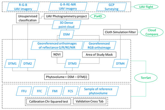
Figure 6.
Flowchart of the applied methodology. Digital terrain models (DTMs) numbered from one to four were used to obtain the FFU, FFC, FMI, and FCS estimators, respectively.
2.9. UAV-Photogrammetric Products
A total of 242 visible images, about 99% of which were calibrated, and 968 multispectral images, 97% of which were calibrated, were processed. In the bundle adjustment process, a median of 76,600 key points per image were identified in the visible images dataset, and close to 53,530 keypoints were identified per multispectral image. All the visible and multispectral orthoimages produced were resampled to a GSD of 2 cm and georeferenced with an RMS error of 1.9 cm.
The shutter speed was constant and sufficient to reach a transversal and longitudinal overlap of 70% and 55%, respectively, distributed in 11 flight paths. Thus, all the pixels belonging to the study area were registered in at least five images.
Visible and multispectral sensors were post-calibrated based on the previous internal calibration by the manufacturer, including the distortion parameters, focal length, centre, and size of the sensors. For co-registration of the multispectral images, the camera models of the four channels were referenced to a unique reference using a median of 5089 matches between each pair of channels.
The photogrammetric project was referenced to the official coordinate system in Spain (ETRS89), UTM zone 30, northern hemisphere, using elevations with respect to MSL. The geoid model was EGM08, and the accuracies obtained from RTX post-processing were 1.8, 3.4, and 1.1 cm in the X, Y, and Z coordinates, respectively.
The first partial result obtained from the photogrammetric project was a dense point cloud (Figure 7) composed of 25.13 million 3D points irregularly distributed, which implies an average density of 352.57 points/m3.
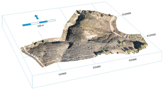
Figure 7.
Perspective view of the dense point cloud, centred in the study area and represented as an RGB composite.
By connecting all the points of the cloud, a TIN was generated by Poisson surface reconstruction [47], which considers all the points at once, thus reducing data noise. The resulting TIN was composed of 12.7 million vertices and 25.3 million facets.
The DSM was obtained by applying an inverse distance weighting method to interpolate a regular 2 cm matrix that evolves to canopy and bare soil. Two filters were applied to remove noise and smooth the surface [34,42].
With this information, the RGB orthoimage and four orthoimages in reflectance units corresponding to the multispectral channels were orthorectified (Figure 8). All these products were georeferenced and saved in GeoTIFF format.
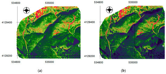
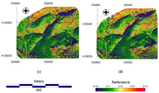
Figure 8.
(a) Green, (b) red, (c) red edge, and (d) near-infrared (NIR) orthoimages corresponding to reflectance, represented in an eight-bits quantitative scale.
3. Results
3.1. Phytovolume Estimation
The FFU and FFC DTMs were interpolated in a regular matrix of 10 cm pixels. When the FMI method was applied, the maximum NDVI in the sample soil area was 0.35. This value was used as a threshold to reclassify the NDVI map as vegetation for pixels with NDVI higher than 0.35 and non-vegetation otherwise (Figure 9). Interpolation of the soil point cloud produced the FMI DTM, resampled with pixels of 2 cm.
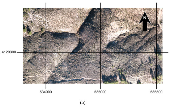
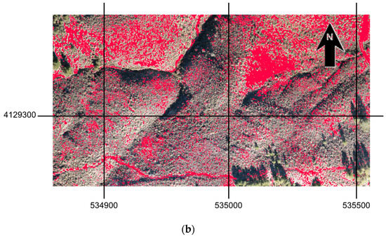
Figure 9.
(a) Detail of the RGB orthoimage composition; (b) non-vegetation points detected by masking the dense point cloud with a threshold NDVI map.
The set parameters that controlled the extract ground points process by the FCS method were the 0.4 m cloth resolution or cloth grid size, the maximum number of 500 terrain simulations, and the 0.1 m threshold for classification. The classification threshold refers to a threshold to classify the point clouds into ground and non-ground parts based on the distances between points and the simulated terrain. Close to 41.4% of the points were classified as ground points.
In the four described cases, the difference between DSM and DTMs provided raster maps where each pixel represents the height of the vegetation. By multiplying these values by the surface associated with a 2 cm2 pixel, four raster maps representing phytovolume estimators were obtained (Figure 10).
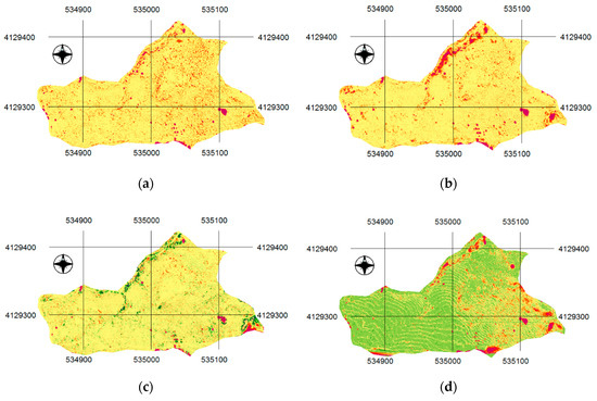
Figure 10.
Phytovolume estimator maps expressed as vegetation height in m based on (a) unclassified dense point cloud (FFU), (b) classified dense point cloud (FFC), (c) multispectral vegetation index (FMI), and (d) cloth simulation filter (FCS).
3.2. Qualitative and Quantitative Analysis
Two types of result analyses were carried out: Qualitative, to determine the ability of the estimators for detecting vegetation areas, and quantitative, to evaluate the estimation of phytovolume accuracy. The qualitative analysis involved three steps. The first was extracting vegetation groups from the four estimators and reclassifying the difference maps between DSM and the four DTMs. Values close to zero were considered soil; up to 1.5 m, shrubs; and more than 1.5 m, trees (Figure 11).
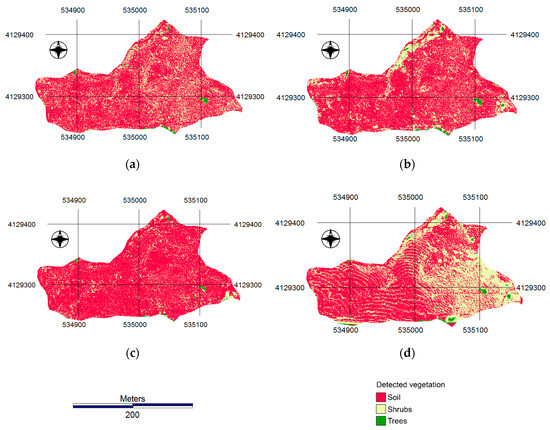
Figure 11.
Vegetation areas detected by (a) unclassified dense point cloud (FFU), (b) classified dense point cloud (FFC), (c) multispectral vegetation index (FMI), and (d) cloth simulation filter (FCS).
Second, the statistical significance of the difference between vegetation masses detected was determined using the McNemar chi-squared test with the proportion of joining classes. Tests showed evidence of differences between all the possible pairwise comparisons of vegetation detected with 95% confidence, except between FFU and FMI.
Third, the four vegetation areas detected were compared to observed classes, delineated by photointerpretation. The similarity between reference data and each of the estimators was evaluated through the corresponding cross-tabulation of confusion matrices, shown by Table 1. Table 2 shows the resulting kappa and Cramer’s statistics [46,48].

Table 1.
Cross-tabulation of confusion matrices corresponding to vegetation areas detected from four estimators and reference data.
Table 2.
Kappa/Cramer’s V of cross-tabulation combinations of vegetation areas detected and reference data confusion matrices.
A higher similarity with the reference data was presented by FMI and FFU, while FFC and FCS did not reach levels that could be considered similar to the reference, due to Cramer’s values decreasing below 0.6.
Some studies were carried out regarding the quantitative analysis to establish the ability for phytovolume estimation. First, all the pairwise comparisons between the phytovolume estimators, as defined in Figure 10, were considered, and the six possible differences between them were calculated. A sample of 2860 data points was extracted from each of the differences, verifying that the distribution was normal with the Kolmogorov–Smirnov test [46,48] at 95% confidence. To quantify the differences between estimator pairs, a classified standardised difference image was created for each pair difference, with z-scores divided into six classes of variance (Figure 12).
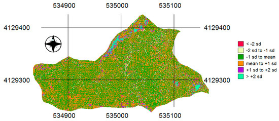
Figure 12.
Classified standard difference image between FFU and FFC with z-scores divided into six classes of variance.
Considering those zones with a z-score higher than two variances to be significant changes, not one of the possible comparisons presented significant differences except those between FFU and FFC, in which 11.12% of the study area showed a z-score higher than two variances.
However, a qualitative comparison of the four phytovolume estimators with the in situ observed phytovolume reference in 768 sample data points was undertaken. The RMSE obtained were 12.3 m, 17.6 m, 66.3 m, and 78.2 m for FMI, FFU, FFC, and FCS, respectively. These ranks suggest that the characteristic radiometric behaviour of the pixels belonging to the canopy is the most efficient tool for separating bare soil and vegetation points and hence generate an accurate DTM.
4. Discussion
The order of magnitude of the global agreement obtained in this work was the same as in previous studies based on biomass estimations using LiDAR remote sensing [3]. Some authors, like [7], determined a global agreement of 76% to 85% when using fused satellite images with LiDAR for fuel-type detection. Logistic regression coefficients close to 70% for modelling fire danger based on satellite imagery were found by [20]. With similar material used in the present work, several fire severity indices were evaluated by [27] based on UAV data with a kappa of 0.536.
From a practical point of view, FFU and FFC obtain the DTMs from the photogrammetric project. However, while FFU does not need postprocessing, a dense point cloud classification process must be carried out in FFC. In order to automate the classification, an unsupervised algorithm based on the frequency of each class was applied, and five target classes were established. On the other hand, morphological analysis of the DSM for extracting DTMs in the cases of FFU and FFC is highly influenced by the scale factor, which has been described as a frequent source of error.
The main advantage of FMI comes from the vegetation index chosen, which is able to accurately detect vegetated areas. However, the need of near infrared information limits the use of UAV on-board cameras working on the visible spectrum. Furthermore, dead vegetation tends to be excluded from phytovolume estimation, although this effect was not significant in this work.
One of the main practical difficulties of FCS is setting the correct parameters of the mathematical model in each type of terrain. Results of FCS mainly depend on a threshold value to classify the point clouds into ground and non-ground parts, based on the distances between points and the simulated terrain. In future works, a sensibility analysis could establish the threshold value with better results, and supervised classifications could be applied to adapt the phytovolume estimation to each case of study. Particularly, pixel-based classification by Neural Network and Object Based Image Analysis could separate vegetated and non-vegetation areas with higher accuracy, and even recognition of individual species.
Using radar and satellite data, regression coefficients between 0.6 and 0.9 for biomass modelling were reported by [18], and fuel-type maps from satellite data with an overall accuracy of 74% were calculated by [19]. The novelty of the indirect estimations obtained in this study is related to the UAV data characteristics: High efficiency and flexibility to adapt the accuracy in each case. Compared to LiDAR, the volume of UAV data is lower. The manpower needed to obtain phytovolume estimation based on UAV data is lower than that of the manual sample, and UAV allows for work in forests with limited accessibility at a reasonable cost.
5. Conclusions
According to the obtained results in the Mediterranean forest in this work, FMI was the best phytovolume estimator, showing the lowest RMSE calculated with the in situ reference data observed at 768 sample sites grouped in four parcels of 500 m2.
The FMI model was the best for detecting vegetated areas, showing statistically significant differences, with respect to the other estimators at a confidence level of 95%.
Estimating the surface occupied by shrubs obtained from FFU, FFC and FCS were compared with FMI, concluding that FMI–FFU comparison presents the best similarity among all the possible pairwise comparisons.
In absolute terms, FMI is the method that best estimates the surface occupied by vegetation compared to the vegetation surface observed by photointerpretation and supervised classification.
In relative terms and considering all the possible pairwise comparisons of phytovolume estimation, differences between them are lower than two variances, except between FFU and FFC.
The use of FMI based on UAV data provides accurate phytovolume estimations that can be applied to several environment management activities, including wildfire prevention. Multitemporal phytovolume estimations could help to model the evolution of forest resources in a very realistic way.
Author Contributions
The contributions of the authors were: Conceptualization, F.C.-R. and J.M.P.R.S.; methodology, F.C.-R., F.A.-V., and P.M.-C.; software P.M.-C. and F.A.-V.; validation, J.M.P.R.S.; formal analysis, F.C.-R. and F.A.-V.; investigation, F.C.-R.; resources, P.M.-C.; data curation, F.C.-R. and P.M.-C.; writing—original draft preparation, F.C.-R.; writing—review and editing, J.M.P.R.S.; visualization, F.C.-R.; project administration, F.A.-V.; funding acquisition, F.A.-V.
Funding
This research received no external funding.
Acknowledgments
Authors give thanks to firemen, security staff, and other technical personnel belonging to Centro Operativo Provincial contra Incendios Forestales de Almería, Plan INFOCA, Consejería de Agricultura, Ganadería, Pesca y Desarrollo Sostenible de la Junta de Andalucía, for their work at the prescribed fire operation. Likewise, thanks to Peripheral Service of Research and Development based on drones, University of Almería, Spain, and Instituto de Ciências Agrárias e Ambientais Mediterrânicas, Évora, Portugal.
Conflicts of Interest
The authors declare no conflict of interest. The funders had no role in the design of the study; in the collection, analyses, or interpretation of data; in the writing of the manuscript, or in the decision to publish the results.
References
- Miao, Z.; Xing-Ying, Z.; Rui-Xia, L.; Lie-Qun, H. A Study of the Validation of Atmospheric CO2 from Satellite Hyper Spectral Remote Sensing. Adv. Clim. Chang. Res. 2014, 5, 131–135. [Google Scholar]
- Goetz, S.; Dubayah, R. Advances in remote sensing technology and implications for measuring and monitoring forest carbon stocks and change. Carbon Manag. 2011, 2, 231–244. [Google Scholar] [CrossRef]
- Zolkos, S.G.; Goetz, S.J.; Dubayah, R. A meta-analysis of terrestrial aboveground biomass estimation using lidar remote sensing. Remote Sens. Environ. 2013, 128, 289–298. [Google Scholar] [CrossRef]
- Navarro, R.M. Fitomasa aérea en los ecosistemas de matorral en el monte Can Vilallonga (T.M. DE Cassà de la Selva-Girona). Ecología 2004, 18, 99–112. [Google Scholar]
- Cerrillo, R.M.N.; Oyonarte, P.B. Estimation of above-ground biomass in shrubland ecosystems of southern Spain. Investig. Agrar. Sist. y Recur. For. 2006, 15, 197–207. [Google Scholar] [CrossRef]
- Swatantran, A.; Dubayah, R.; Roberts, D.; Hofton, M.; Blair, J.B. Mapping biomass and stress in the Sierra Nevada using lidar and hyperspectral data fusion. Remote Sens. Environ. 2011, 115, 2917–2930. [Google Scholar] [CrossRef]
- Alonso-Benito, A.; Arroyo, L.A.; Arbelo, M.; Hernández-Leal, P. Fusion of WorldView-2 and LiDAR data to map fuel types in the Canary Islands. Remote Sens. 2016, 8, 669. [Google Scholar] [CrossRef]
- Saǧlam, B.; Bilgili, E.; Durmaz, B.D.; Kadioǧullari, A.I.; Kücük, Ö. Spatio-temporal analysis of forest fire risk and danger using Landsat imagery. Sensors 2008, 8, 3970–3987. [Google Scholar] [CrossRef]
- Baeza, M.J.; Raventós, J.; Escarré, A.; Vallejo, V.R. Fire risk and vegetation structural dynamics in Mediterranean shrubland. Plant Ecol. 2006, 187, 189–201. [Google Scholar] [CrossRef]
- Wells, T.C.E. Ecosystems of the World II: Mediterranean-type Shrublands, Edited by F. Di Castri, D.W. Goodall & R.L. Specht. Elsevier Scientific Publishing Company, Amsterdam–Oxford–New York: xii + 643 pp., with numerous text-figures and tables, 27 × 20 × 38 cm, clothbound, US $136.50, Dfl. 280, 1981. Environ. Conserv. 1984, 11, 192–193. [Google Scholar]
- Le, A.V.; Paull, D.J.; Griffin, A.L. Exploring the inclusion of small regenerating trees to improve above-ground forest biomass estimation using geospatial data. Remote Sens. 2018, 10, 1446. [Google Scholar] [CrossRef]
- González-Jaramillo, V.; Fries, A.; Zeilinger, J.; Homeier, J.; Paladines-Benitez, J.; Bendix, J. Estimation of above ground biomass in a tropical mountain forest in southern Ecuador using airborne LiDAR data. Remote Sens. 2018, 10, 660. [Google Scholar] [CrossRef]
- Knapp, N.; Huth, A.; Kugler, F.; Papathanassiou, K.; Condit, R.; Hubbell, S.P.; Fischer, R. Model-assisted estimation of tropical forest biomass change: A comparison of approaches. Remote Sens. 2018, 10, 731. [Google Scholar] [CrossRef]
- Enguita, I.D.; Jarauta, M.J.O.; Ferré, A.A.; Calvo, L.L.; Pérez, F.M. Descripción Y Evaluación De La Fitomasa Presente En Áreas No Cultivadas De La Comarca De Monegros (Aragón). Pastos 1995, 25, 87–97. [Google Scholar]
- Clark, M.L.; Roberts, D.A.; Ewel, J.J.; Clark, D.B. Estimation of tropical rain forest aboveground biomass with small-footprint lidar and hyperspectral sensors. Remote Sens. Environ. 2011, 115, 2931–2942. [Google Scholar] [CrossRef]
- Armand, D.; Etienne, M.; Legrand, C.; Marechal, J.; Valette, J.C. Shrub biomass, bulk volume and structure in the French Mediterranean region. Ann. Des. Sci. For. 1993, 50, 79–89. [Google Scholar] [CrossRef][Green Version]
- Mancilla-Leytón, J.M.; Pino Mejías, R.; Martín Vicente, A. Do goats preserve the forest? Evaluating the effects of grazing goats on combustible Mediterranean scrub. Appl. Veg. Sci. 2013, 16, 63–73. [Google Scholar] [CrossRef]
- Collingwood, A.; Treitz, P.; Charbonneau, F.; Atkinson, D.M. Artificial neural network modeling of high arctic phytomass using synthetic aperture radar and multispectral data. Remote Sens. 2014, 6, 2134–2153. [Google Scholar] [CrossRef]
- Mallinis, G.; Galidaki, G.; Gitas, I. A comparative analysis of EO-1 hyperion, quickbird and landsat TM imagery for fuel type mapping of a typical mediterranean landscape. Remote Sens. 2014, 6, 1684–1704. [Google Scholar] [CrossRef]
- Bisquert, M.; Sánchez, J.M.; Caselles, V. Modeling fire danger in Galicia and asturias (Spain) from MODIS images. Remote Sens. 2013, 6, 540–554. [Google Scholar] [CrossRef]
- Cartus, O.; Santoro, M.; Wegmüller, U.; Rommen, B. Benchmarking the Retrieval of Biomass in Boreal Forests Using P-Band SAR Backscatter with Multi-Temporal C- and L-Band Observations. Remote Sens. 2019, 11, 1695. [Google Scholar] [CrossRef]
- Huang, X.; Ziniti, B.; Torbick, N.; Ducey, M.J. Assessment of forest above ground biomass estimation using multi-temporal C-band Sentinel-1 and Polarimetric L-band PALSAR-2 data. Remote Sens. 2018, 10, 1424. [Google Scholar] [CrossRef]
- Doughty, C.L.; Cavanaugh, K.C. Mapping coastal wetland biomass from high resolution unmanned aerial vehicle (UAV) imagery. Remote Sens. 2019, 11, 540. [Google Scholar] [CrossRef]
- Zhang, H.; Sun, Y.; Chang, L.; Qin, Y.; Chen, J.; Qin, Y.; Du, J.; Yi, S.; Wang, Y. Estimation of grassland canopy height and aboveground biomass at the quadrat scale using unmanned aerial vehicle. Remote Sens. 2018, 10, 851. [Google Scholar] [CrossRef]
- Richards, J.A. Remote Sensing Digital Image Analysis, 5th ed.; Springer: Berlin, Germany, 2013; ISBN 978-3-642-30062-2. [Google Scholar]
- Fernández-Guisuraga, J.M.; Sanz-Ablanedo, E.; Suárez-Seoane, S.; Calvo, L. Using unmanned aerial vehicles in postfire vegetation survey campaigns through large and heterogeneous areas: Opportunities and challenges. Sensors 2018, 18, 586. [Google Scholar] [CrossRef]
- Carvajal-Ramírez, F.; da Silva, J.R.M.; Agüera-Vega, F.; Martínez-Carricondo, P.; Serrano, J.; Moral, F.J. Evaluation of fire severity indices based on pre- and post-fire multispectral imagery sensed from UAV. Remote Sens. 2019, 11, 993. [Google Scholar] [CrossRef]
- Dash, J.P.; Pearse, G.D.; Watt, M.S. UAV multispectral imagery can complement satellite data for monitoring forest health. Remote Sens. 2018, 10, 1216. [Google Scholar] [CrossRef]
- Fonstad, M.A.; Dietrich, J.T.; Courville, B.C.; Jensen, J.L.; Carbonneau, P.E. Topographic structure from motion: A new development in photogrammetric measurement. Earth Surf. Process. Landf. 2013, 38, 421–430. [Google Scholar] [CrossRef]
- Furukawa, Y.; Ponce, J. Accurate, Dense, and Robust Multiview Stereopsis. IEEE Trans. Pattern Anal. Mach. Intell. 2010, 32, 1362–1376. [Google Scholar] [CrossRef]
- Agüera-Vega, F.; Carvajal-Ramírez, F.; Martínez-Carricondo, P.J. Accuracy of Digital Surface Models and Orthophotos Derived from Unmanned Aerial Vehicle Photogrammetry. J. Surv. Eng. 2016, 143, 1–10. [Google Scholar] [CrossRef]
- Martínez-Carricondo, P.; Agüera-Vega, F.; Carvajal-Ramírez, F.; Mesas-Carrascosa, F.-J.; García-Ferrer, A.; Pérez-Porras, F.-J. Assessment of UAV-photogrammetric mapping accuracy based on variation of ground control points. Int. J. Appl. Earth Obs. Geoinf. 2018, 72, 1–10. [Google Scholar] [CrossRef]
- Agüera-Vega, F.; Carvajal-Ramírez, F.; Martínez-Carricondo, P.; Sánchez-Hermosilla López, J.; Mesas-Carrascosa, F.J.; García-Ferrer, A.; Pérez-Porras, F.J. Reconstruction of extreme topography from UAV structure from motion photogrammetry. Meas. J. Int. Meas. Confed. 2018, 121, 127–138. [Google Scholar] [CrossRef]
- Becker, C.; Häni, N.; Rosinskaya, E.; D’Angelo, E.; Strecha, C. Classification of Aerial Photogrammetric 3D Point Clouds. ISPRS Ann. Photogramm. Remote Sens. Spat. Inf. Sci. 2017, 4, 3–10. [Google Scholar] [CrossRef]
- Zhang, W.; Qi, J.; Wan, P.; Wang, H.; Xie, D.; Wang, X.; Yan, G. An easy-to-use airborne LiDAR data filtering method based on cloth simulation. Remote Sens. 2016, 8, 501. [Google Scholar] [CrossRef]
- Junta de Andalucía Interreg-Sudoe OPEN2PRESERVE. Available online: https://open2preserve.eu/estudi/experiencia-piloto-en-andalucia/ (accessed on 13 March 2019).
- Gobierno de España La Red Natura 2000 en España. Available online: https://www.miteco.gob.es/es/biodiversidad/temas/espacios-protegidos/red-natura-2000/rn_espana.aspx (accessed on 13 March 2019).
- Parrot Drones SAS Parrot Sequoia. Available online: https://www.parrot.com/soluciones-business/profesional/parrot-sequoia#parrot-sequoia- (accessed on 13 March 2019).
- SPH Engineering SIA UgCS Mission Planning Sofware for UAV Professionals. Available online: https://www.ugcs.com/ (accessed on 13 March 2019).
- Aguilar, F.J.; Agüera, F.; Aguilar, M.A.; Carvajal, F. Effects of Terrain Morphology, Sampling Density, and Interpolation Methods on Grid DEM Accuracy. Photogramm. Eng. Remote Sens. 2005, 71, 805–816. [Google Scholar] [CrossRef]
- Glocker, M.; Landau, H.; Leandro, R.; Nitschke, M. Global precise multi-GNSS positioning with trimble centerpoint RTX. In Proceedings of the 2012 6th ESA Workshop on Satellite Navigation Technologies (Navitec 2012) & European Workshop on GNSS Signals and Signal Processing, Noordwijk, The Netherlands, 5–7 December 2012; pp. 1–8. [Google Scholar]
- Pix4D SA Pix4D Make Better Decisions with Accurate 3D Maps and Models. Available online: https://www.pix4d.com/ (accessed on 13 March 2019).
- Huesca, M.; Merino-de-Miguel, S.; González-Alonso, F.; Martínez, S.; Miguel Cuevas, J.; Calle, A. Using AHS hyper-spectral images to study forest vegetation recovery after a fire. Int. J. Remote Sens. 2013, 34, 4025–4048. [Google Scholar] [CrossRef]
- Dowhower, S.L.; Teague, W.R.; Ansley, R.J.; Pinchak, W.E. Dry-Weight-Rank Method Assessment in Heterogenous Communities. J. Range Manag. 2007, 54, 71. [Google Scholar] [CrossRef]
- George, M.R.; Laca, E.A.; Barry, S.J.; Larson, S.R.; McDougald, N.K.; Ward, T.A.; Harper, J.M.; Dudley, D.M.; Ingram, R.S. Comparison of comparative yield and stubble height for estimating herbage standing crop in annual rangelands. Rangel. Ecol. Manag. 2006, 59, 438–441. [Google Scholar] [CrossRef]
- Foody, G.M. Thematic Map Comparison: Evaluating the Statistical Significance of Differences in Classification Accuracy. Photogramm. Eng. Remote Sens. 2004, 70, 627–633. [Google Scholar] [CrossRef]
- Kazhdan, M.; Bolitho, M.; Hoppe, H. Poisson Surface Reconstruction. In Proceedings of the Eurographics Symposium on Geometry Processing, Cagliari, Italy, 26–28 June 2006; Eurographics Association: Aire-la-Ville, Switzerland; pp. 61–70. [Google Scholar]
- Acock, A.C.; Stavig, G.R. A Measure of Association for Nonparametric Statistics. Soc. Forces 1979, 57, 1381–1386. [Google Scholar] [CrossRef]


© 2019 by the authors. Licensee MDPI, Basel, Switzerland. This article is an open access article distributed under the terms and conditions of the Creative Commons Attribution (CC BY) license (http://creativecommons.org/licenses/by/4.0/).