Modeling Quiet Solar Luminosity Variability from TSI Satellite Measurements and Proxy Models during 1980–2018

Abstract

A continuous record of direct total solar irradiance (TSI) observations began with a series of satellite experiments in 1978. This record requires comparisons of overlapping satellite observations with adequate relative precisions to provide useful long term TSI trend information. Herein we briefly review the active cavity radiometer irradiance monitor physikalisch-meteorologisches observatorium davos (ACRIM-PMOD) TSI composite controversy regarding how the total solar irradiance (TSI) has evolved since 1978 and about whether TSI significantly increased or slightly decreased from 1980 to 2000. The main question is whether TSI increased or decreased during the so-called ACRIM-gap period from 1989 to 1992. There is significant discrepancy between TSI proxy models and observations before and after the gap, which requires a careful revisit of the data analysis and modeling performed during the ACRIM-gap period. In this study, we use three recently proposed TSI proxy models that do not present any TSI increase during the ACRIM-gap, and show that they agree with the TSI data only from 1996 to 2016. However, these same models significantly diverge from the observations from 1981 and 1996. Thus, the scaling errors must be different between the two periods, which suggests errors in these models. By adjusting the TSI proxy models to agree with the data patterns before and after the ACRIM-gap, we found that these models miss a slowly varying TSI component. The adjusted models suggest that the quiet solar luminosity increased from the 1986 to the 1996 TSI minimum by about 0.45 W/m² reaching a peak near 2000 and decreased by about 0.15 W/m² from the 1996 to the 2008 TSI cycle minimum. This pattern is found to be compatible with the ACRIM TSI composite and confirms the ACRIM TSI increasing trend from 1980 to 2000, followed by a long-term decreasing trend since.

1. Introduction

The total solar irradiance (TSI) is the solar energy flux density outside the Earth’s atmosphere at a distance from the sun of 1 astronomical unit (AU), given in SI units of Watts per square meter (W/m²). The quiet solar luminosity variability on decadal to millennial timescales is still highly uncertain and is still the subject of much debate [1,2,3,4,5,6,7,8,9,10,11,12].

The quiet solar luminosity could undergo a significant decadal to millennial timescale variation because during the Maunder minimum (1645–1715), despite the near disappearance of sunspots, heliospheric activity was still significantly varying [13,14]. TSI proxy models attempting to take into account this behavior reproduce a large TSI variability both during the Maunder minimum and from 1700 to the present time between 3 and 6 W/m² [1,2,8,12]. Conversely, other recent TSI proxy models such as naval research laboratory total solar irradiance 2 (NRLTSI2) [15] and spectral and total irradiance reconstructions-S (SATIRE-S) [16] show a nearly flat TSI variability during the Maunder minimum and a TSI increase between then and the December 2008–2009 TSI cycle minimum of as low as 0.6 W/m² and 0.1 W/m², respectively [3,12] (Appendix B lists the definition of all acronyms used in this paper).

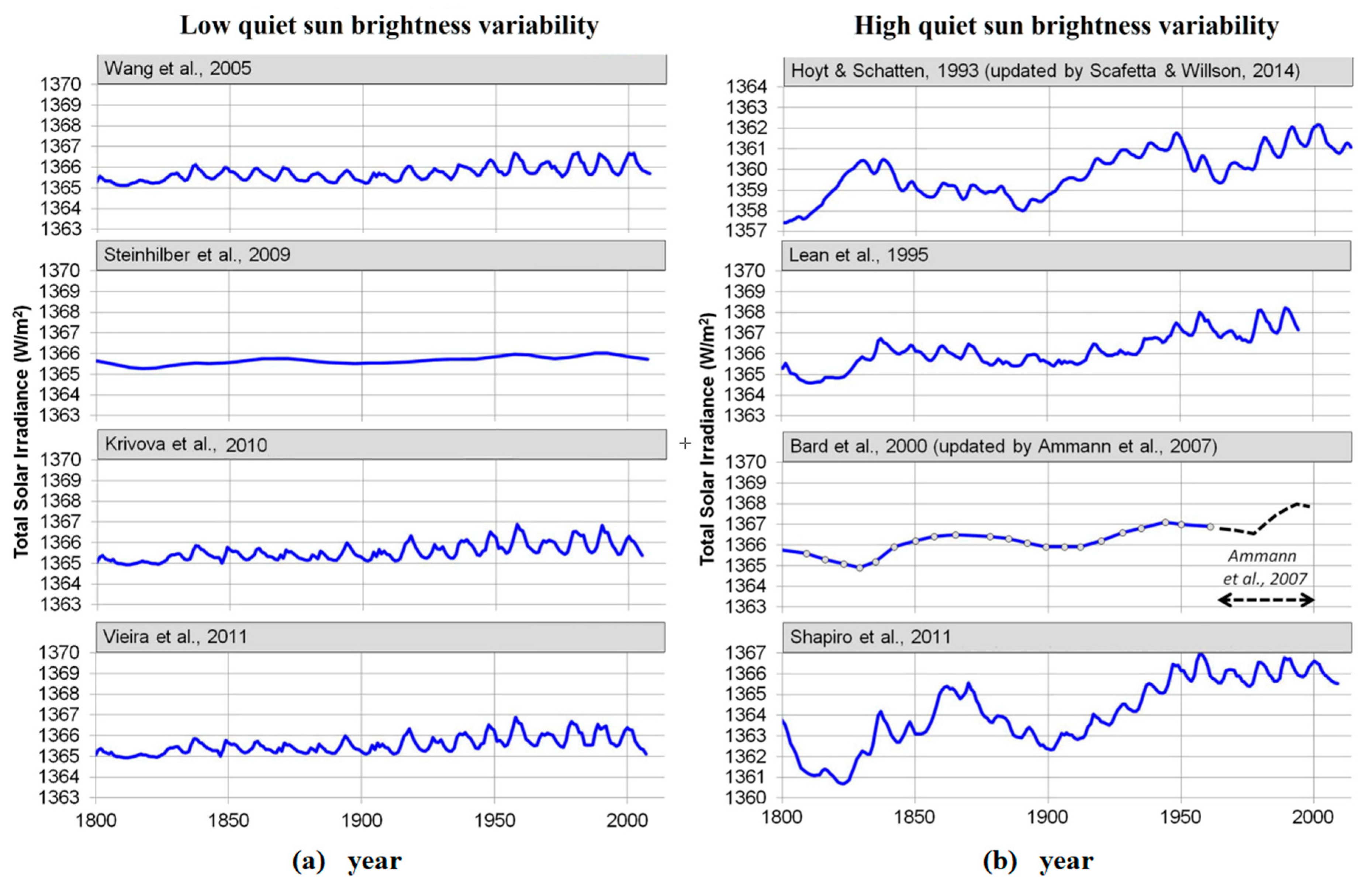
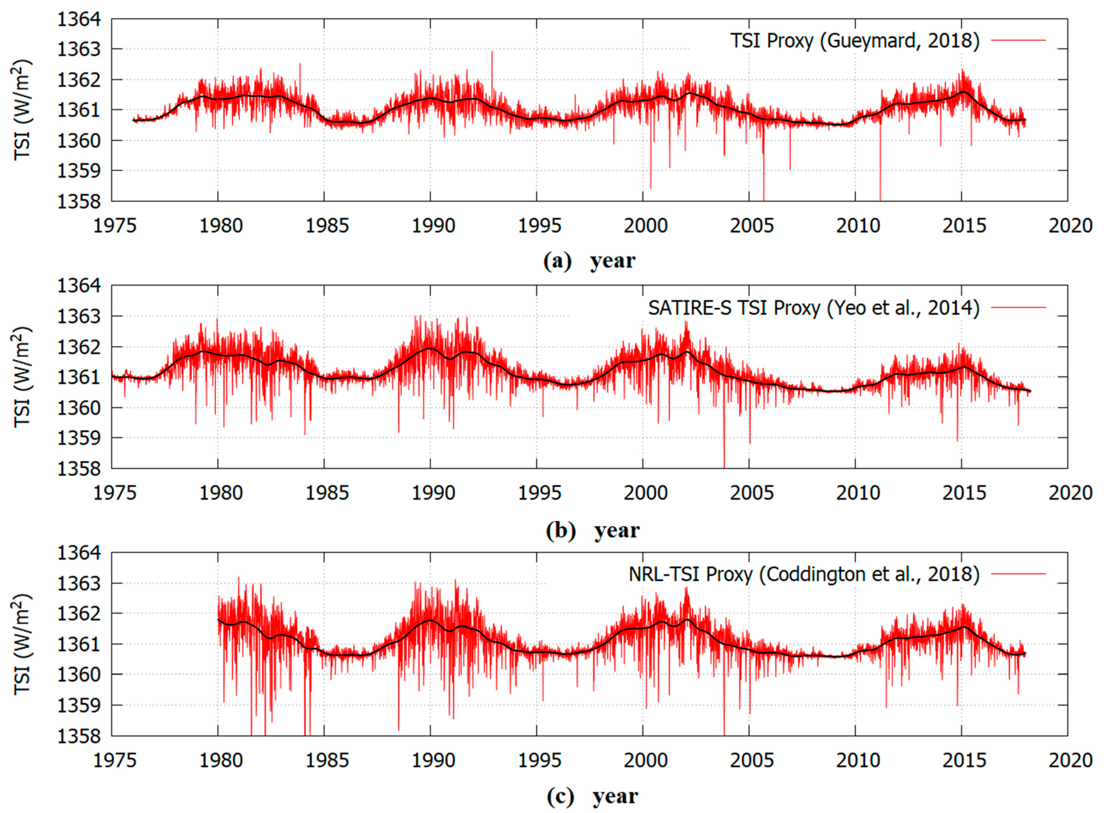
Figure 1 shows examples of proposed TSI models characterized by a low or a high quiet solar luminosity variability. Solving this uncertainty is necessary for properly assessing the solar minimum-to-minimum trend, which is essential for understanding how solar activity evolves and its relationship to variability in the Earth’s climate [17,18,19,20,21,22,23]. The eight records are depicted using a window of 7 W/m² to facilitate a visual comparison to highlight the difference in their secular variability.

The low decadal-to-millennial timescale variability observed in some TSI proxy models [15,16,24] is likely due to the chosen model constructors that stress the time evolution of sunspot darkening, coronal mass ejections, facular brightening, and photospheric magnetism. These features are described by records such as the daily MgII index (at 280 nm, a proxy representative for the UVC and UVB spectral solar irradiance variability), radio flux record (at 10.7 cm, whose radiation comes from the high chromosphere and low corona and is generated by thermal Bremsstrahlung and gyro-radiation) and sunspot number and area records. However, these indices are mostly representative of the active regions of the sun such as photospheric sunspots and faculae and may poorly model the variability of the quiet solar luminosity that involves global solar changes. In fact, the chosen proxy records show a very small solar cycle minimum-to-minimum variability because very few sunspots and faculae are observed during solar cycle minima. Therefore, during such minima those records are bounded to the limit value of zero. On the contrary, according to some early study [25], a TSI secular variation could also approach a 0.5%–1.0% over the past century, given the low precision of pre-1978 pyrheliometry and insufficient understanding of internal solar radiative physics.

The proper way to measure and evaluate the quiet solar luminosity variability is through direct TSI satellite observations and, in particular, through the analysis of the solar cycle minimum-to-minimum trending observed in their composites. However, the long-term trend in the TSI satellite records, available since 1978, remains also a scientific uncertainty that requires careful examination of the relevant issues from various perspectives. Two main factors explain this persisting disagreement: (1) the direct TSI satellite database is relatively short, ~40 years since 1978, and it is made of discontinuous records as depicted in Figure 2 and (2) the proxy models cannot be properly evaluated and calibrated against the TSI observations due both to the shortness of the TSI satellite composite records and to the uncertainties in their solar cycle minimum-to-minimum trends, particularly from 1986 to 1996 [26,27,28].

The scientific debate on this issue has become known as the active cavity radiometer irradiance monitor physikalisch-meteorologisches observatorium davos (ACRIM-PMOD) controversy and will be briefly reviewed in Section 2. The main issue is whether TSI increased or decreased during the so-called ACRIM-gap period from 1989 to 1991. The ACRIM-Gap is the late 1989 to late 1991 period following the end of the solar maximum mission (SMM)/ACRIM1 and the start of the upper atmosphere research satellite (UARS)/ACRIM2 experiments during which time there were no high accuracy/precision TSI monitoring satellite experiments (http://acrim.com).

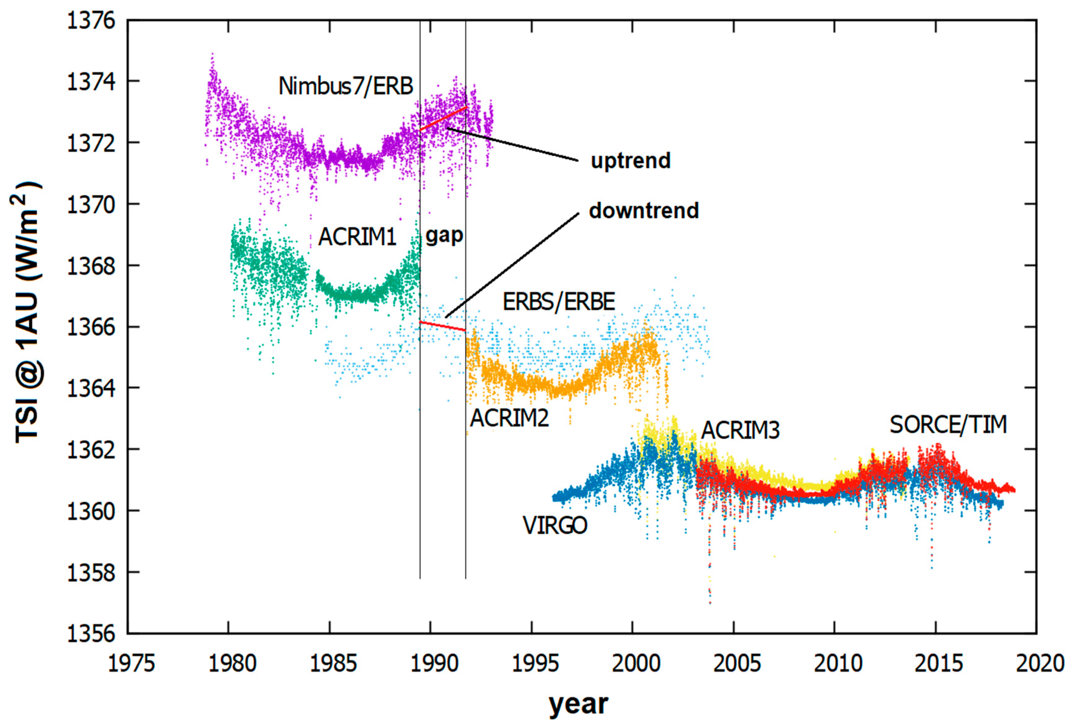
Figure 2 compares the main TSI satellite records from 1978 to 2018. The most relevant ones are: SMM/ACRIM1 (1980–1989), UARS/ACRIM2 (1991–2001) and ACRIMSAT/ACRIM3 (1999–2013) [26,29,30], Nimbus7/Earth radiation budget (ERB; 1978–1993) [31], Earth radiation budget satellite/Earth radiation budget experiment (ERBS/ERB; 1984–2003) [32], solar and heliospheric observatory/variability of solar irradiance and gravity oscillations (SOHO/VIRGO; 1996–present) [27,33] and solar radiation and climate experiment/total irradiance monitor (SORCE/TIM; 2003–present) [10,34].

Several TSI satellite composites have been proposed: ACRIM [26], PMOD [33,35], RMIB [36] and those suggested by Scafetta [37] and Dudok de Wit et al. [28]. Although these composites use different sets of TSI satellite records and merging methodologies, they are relatively equivalent since about 1992, the beginning of the ACRIM2 record, because they are all based on high-quality TSI observations. Yet, as clarified below, PMOD used their own modified versions of the original results compiled by the experiment teams for the SMM/ACRIM1, UARS/ACRIM2 and Nimbus7/ERB records to cover the period 1978–1992 and, therefore, its proposed record cannot be considered a real TSI satellite composite but a model construction. The ACRIM-PMOD controversy is about the scientific legitimacy of such modifications.

Herein we propose an alternative method to evaluate whether a TSI composite of the available satellite records should resemble more closely the ACRIM or PMOD records depicted in Figure 3. We invert the PMOD approach of using TSI models to modify TSI observations and instead use the TSI observations to modify and fine-tune the low-frequency component of the TSI proxy models to determine how they would look if forced to mimic the data.

The proposed approach statistically models the discrepancy between the uncontroversial TSI observations before and after the ACRIM-gap period 1989.53–1991.76 and recent TSI proxy models that do not show a significant TSI minimum to minimum trend. In this way, we can ignore the controversial and low-quality Nimbus7/ERB and ERBS/ERBE records, which are the TSI records mostly responsible for the ACRIM-PMOD controversy, and solve the ACRIM-gap problem without them. We will show that the proxy models are found to exhibit different scaling errors relative to the data between the early and later periods. Then, a regression model can be developed to characterize and compensate for these errors. Finally, the same model can be used to empirically correct both the TSI proxy models and, simultaneously, cross-calibrate the ACRIM1 results with the post ACRIM-gap TSI records. This operation leads to new insights on the quiet solar luminosity variability in the 40+ year TSI record. The proposed solutions are further compared against the available TSI satellite composites to determine which one is the most consistent with the data.

2. A Review of the ACRIM-PMOD Controversy

A large uncertainty exists in the TSI composites during the period from 1978 to 1992. It is mostly due to the fact that the ACRIM2 mission was delayed because of the Space Shuttle Challenger disaster on January 28, 1986, which prevented this record from overlapping with the ACRIM1 record ending in July 1989 (1989.53). The ACRIM-gap (1989.53–1991.76) prevents a direct cross-calibration between the two high-quality ACRIM1 and ACRIM2 TSI records: see Figure 2. ACRIM 1-2-3 records consist of high-quality TSI data made of up to 720 30-s averaged, self-calibrated, shuttered measurements per day [26].

During the ACRIM-gap only results from the lower quality TSI records produced by Nimbus7/ERB and ERBS/ERBE are available. The quality of these TSI observations was limited by a lack of degradation self-calibration capability, by a lack of independent solar pointing and other issues. Moreover, for most of its lifetime, Nimbus7/ERB measured TSI only for a few minutes during each of an average of 14 orbits per day and missed one day every four [31]. ERBS/ERBE was even more limited because it was also constrained to one shuttered observation every 14 days, on average [32].

The main problem is that during the ACRIM-gap, Nimbus7/ERB and ERBS/ERBE records have incompatible trends. Nimbus7/ERB trends up (+0.26 ± 0.04 W/m²yr) while ERBS/ERBE trends down (−0.26 ± 0.15 W/m²yr): see Figure 2 [26,27,30,33,35,38]. Both ACRIM and PMOD science teams agree that during that period at least one of these two TSI records was affected by serious instrumental problems. However, they disagree about which one is the most likely representation of TSI variability and should, therefore, be preferred to bridge ACRIM1 and ACRIM2 records across the gap.

PMOD used TSI proxy model predictions to claim that during the ACRIM-gap period Nimbus7/ERB sensor was affected by an increased sensitivity [2,27,32,33,35,39,40,41]. Consequently, during the gap, PMOD significantly altered the Nimbus7/ERB record downward by about 0.8–0.9 W/m² before connecting ACRIM1 and ACRIM2 [38,42] (Figure 1 and Figure 4). PMOD also made other TSI modifications to the data of the early periods of Nimbus7/ERB, ACRIM1 and ACRIM2, claiming uncorrected sensor degradations. PMOD data modifications were made without examination of original instrumentation, data or data reduction approaches or any detailed consultation with the original satellite experiment science teams. The proposed rationale was that models could be used to fine-tune experimental data. This idea was apparently first proposed in Lean et al. [2] where it was claimed that deviations between TSI data and proxy models “may reflect instrumental effects” alone. Finally, Fröhlich and Lean [35] proposed the first PMOD TSI composite that used Nimbus7/ERB, ACRIM1 and ACRIM2 TSI data they modified using specific TSI proxy model predictions [32,39].

The modification of accurate and precise satellite data using proxy models is a highly questionable approach. ACRIM claims that it is improper to modify published satellite data using virtually un-validated proxy models without detailed knowledge of the satellite instrumentation that only the science teams of the original experiments would likely have. Essentially, a proxy model study that highlights a discrepancy between data and predictions can only suggest the need to investigate a specific case. However, the necessity of adjusting the data and how to do it must still be experimentally justified. By not doing so, the risk is to manipulate the experimental data to support a particular solar model or other bias.

ACRIM contends that the Nimbus7/ERB TSI upward trend during the ACRIM-gap period is more likely correct than the ERBS/ERBE TSI downward trend because it agrees with the solar activity-TSI variability paradigm established by the ACRIM1 experiment [42,43]. In fact, the downward ERBE trend is at variance with the paradigm and was caused by well-documented degradation of its sensors that were experiencing their first exposure to the high UV radiation levels characteristic of solar activity maxima. High UV exposure is known to cause excess degradation of TSI sensors in other satellite results [26,30,42,44]. Nimbus7/ERB experienced a similar excess degradation 11 years earlier during the TSI maximum of solar cycle 21 [38,42] and would have already reached its asymptotic degradation limit during the ACRIM Gap. Clearly, the Nimbus7/ERB TSI record is the most reliable choice to relate the ACRIM1 and ACRIM2 records across the ACRIM-Gap.

However, both the ERB and ERBE TSI records could still contain secondary levels of inaccuracy caused by compromises of their experimental designs and operation, including a lack of independent solar pointing among other issues. The inaccuracy of the Nimbus7/ERB record was tested in Scafetta [37] (Figure 3) where it was determined that on a time scale of about 1–2 years, it could depart from ACRIM1 at most by ±0.2 W/m². This statistical bias is, however, significantly lower than the 0.8–0.9 W/m² drift hypothesized by PMOD. Thus, PMOD modifications of the Nimbus7/ERB record during the ACRIM-gap are statistically implausible and would require very robust experimental justifications that have not been made.

PMOD-proposed modifications of the experimental TSI records have always been uncertain despite their being labeled as “corrections”. Fröhlich and Lean [35] claimed that Nimbus7/ERB had to be adjusted downward because of two presumed “glitches” occurred near October 1, 1989, and May 8, 1990, by −0.26 and −0.32 W/m² respectively. Fröhlich [45] claimed that those same adjustments had to be −0.31 and −0.37 W/m². Fröhlich [41] changed his previous opinion by claiming that the first glitch adjustment, now occurred on September 29, 1989, had to be adjusted with a −0.417 W/m² shift while the second glitch was “difficult to locate” and, therefore, he substituted it with a linear drift model requiring an additional correction of about −0.43 W/m².

Scafetta and Willson [38] examined the PMOD modifications of Nimbus7/ERB. The first event was a postulated “glitch” on September 29, 1989, causing a sudden sensitivity increase that Fröhlich contended required a downward adjustment of −0.47 W/m² on that day. The second event was a postulated sensitivity drift requiring a total adjustment of −0.4 W/m² from 1989.5 to 1992.5. Finally, Fröhlich [46] defended his modifications of Nimbus7/ERB, ACRIM1, and ACRIM2 TSI published records from critiques [37,47] by stressing his 15-year experience with the analysis of the VIRGO radiometers. However, VIRGO was compromised by failure of its shutter mechanisms at launch and required comparison with the other satellite TSI experiments and significant adjustments to provide a proxy to true differentially shuttered results. Additionally VIRGO sensors experienced excessive degradation during its mission that provided another significant source of uncertainty. It is unlikely that the quality of VIRGO results would be adequate to justify alterations of TSI data produced by the other ongoing experiments in which the VIRGO team was not directly involved or had made no significant effort to discuss the issue in detail with the original experiment teams. Thus, the proposed PMOD “corrections” of the Nimbus7/ERB, ACRIM1 and ACRIM2 published TSI records can only be considered conjectures.

In the case of Nimbus7/ERB, tests were performed by its original experimental team that disproved Frohlich’s claims as demonstrated in the supplemental file published in Scafetta and Willson [47]. This supplement includes a testimonial by Dr. Hoyt (the director and technical authority for the Nimbus7/ERB mission) that the claim of a spurious sensitivity increase of the Nimbus7/ERB sensor during the ACRIM-gap was carefully investigated and dismissed from an experimental perspective. Hoyt concluded his testimonial by stating that “Frohlich’s PMOD TSI composite is not consistent with the internal data or physics of the Nimbus7 cavity radiometer” (see Appendix A). The ACRIM science team also evaluated the PMOD alterations of some early ACRIM1 and ACRIM2 published records and found them to be unwarranted because the claimed early degradation of their sensors [2] had been already properly corrected using ACRIM instrumentation sensor redundancy and no further adjustment was required [26] (supplement). The supplement of Ref. [26] also contains a link to a critical testimonial of Willson regarding PMOD modifications of ACRIM1 and ACRIM2 datasets (published in Scafetta [21]). Thus, both Willson and Hoyt, the principal investigators of the ACRIM and Nimbus7/ERB TSI satellite experiments, respectively, are convinced that the PMOD modifications of their TSI published records are unjustified.

In support of Hoyt’s testimony, Scafetta and Willson [38,47] showed that the PMOD’s claims and downward modifications of the Nimbus7/ERB record during the ACRIM-gap are contradicted by numerous pieces of evidence. For example, the PMOD hypothesized 9/29/1989 glitch of the Nimbus7/ERB sensor is contradicted by direct comparison with the ERBS/ERBE record [37,38] and by the fact that the observed divergence between NIMBUS7/ERB and ERBS/ERBE occurred during October and November 1989. Moreover, this event was not instantaneous but gradual: a fact that could be explained by a rapid degradation of the ERBS/ERBE sensor during those months discussed above [37,38].

PMOD’s claim of an anomalous sensitivity increase of the Nimbus7/ERB sensor during the ACRIM-gap was originally proposed by Lee III et al. [32]. These authors claimed that a simple multi-regression TSI proxy model based upon the 10.7-cm solar radio flux (F10) and the photometric sunspot index (PSI) was able to identify TSI variability trends due to drifts or shifts in the spacecraft sensor responses. They found that their TSI proxy model diverged from Nimbus7/ERB during the ACRIM gap and concluded that its experimental data required adjustments. However, it is evident that the Lee III et al. [32] result could also be interpreted as meaning that their TSI proxy model was not able to track the real TSI variability, in particular during a solar maximum period when the quiet solar luminosity could gradually evolve as well. Moreover, as both F10 and PSI indexes are indicative of the active solar regions and do not show any trend between consecutive solar cycle minima, any fit model constructed using them alone would not show any TSI cycle minimum-to-minimum variability by construction. Thus, Lee’s chosen solar model is improper because it lacked the specific physical property—namely the possibility of a solar cycle minimum-to-minimum trending—that would be necessary to test whether the quiet solar luminosity varies or not from a solar cycle to the next. Indeed, TSI proxy models based on PSI and MgII index underestimate TSI observations at the time of solar cycle 21 and 22 maximum and during the beginning of its TSI decline toward solar minimum and, therefore, the validity of these models should not be overstated [48].

In contrast, Scafetta and Willson [38] (Figure 5b) showed that during the ACRIM-gap the Kitt Peak National Solar Observatory solar magnetic field strength (SMFS) trends upward so the solar activity-TSI paradigm would predict a corresponding upward TSI trend, which strongly supports the Nimbus7/ERB upward trend during the same period. Similar conclusions were implied by alternative solar magnetic field strength measurements [38].

It is evident that the result regarding whether during the ACRIM-gap Nimbus7/ERB record is well represented or not by a solar proxy model depends on the specific model or solar observable one chooses. Therefore, the claims by Lean et al. [2], Lee III et al. [32] and Chapman et al. [39], which were later reiterated by PMOD [27,35,40], are doubtful. Other considerations supporting the TSI upward trending between 1980 and 2000, shown by the ACRIM TSI composite, will be briefly discussed in Section 6.

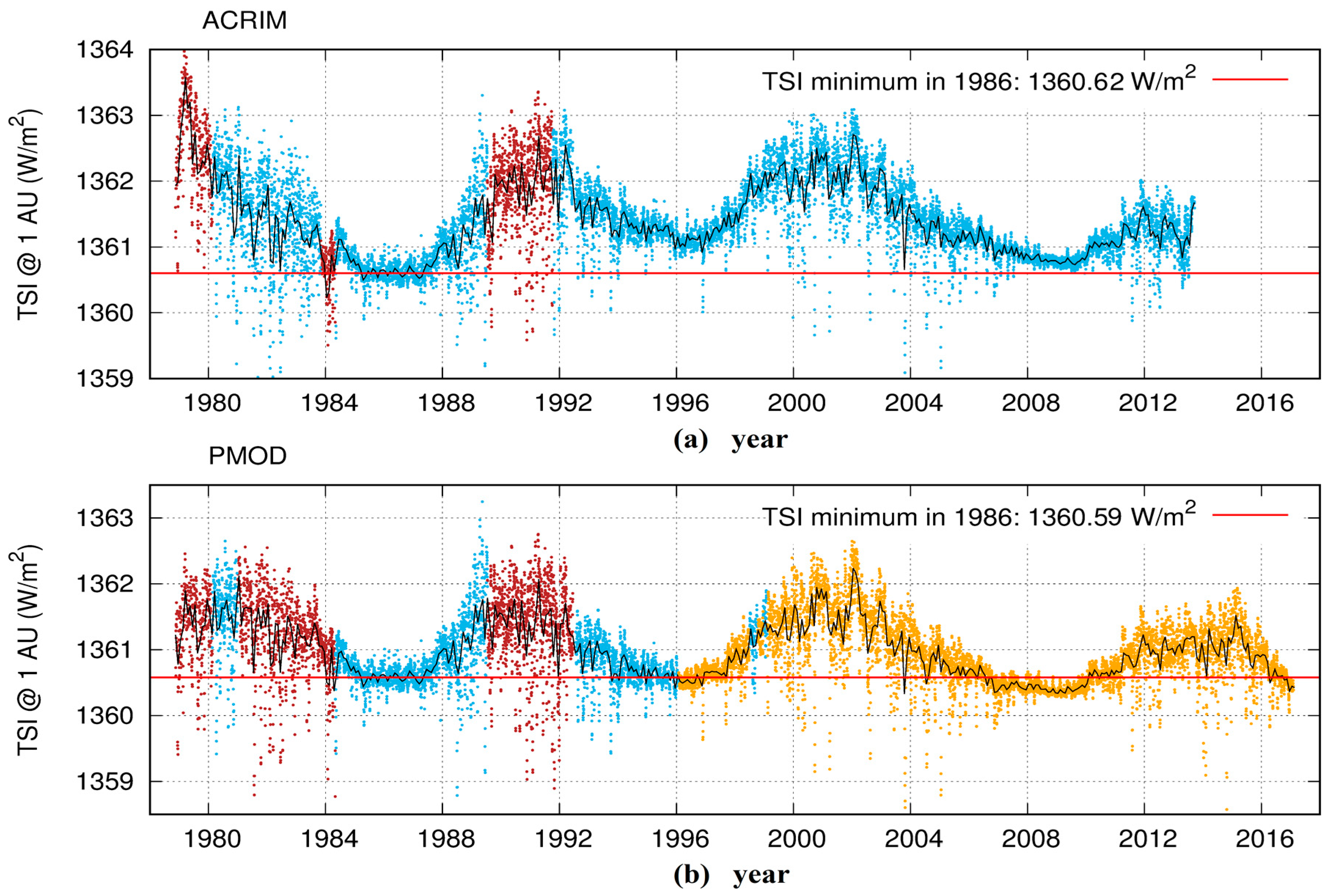
As explained in the introduction, the contrasting claims of ACRIM and PMOD yielded two alternative TSI satellite composites showing a different multi-decadal trending during solar cycles 21–24, as shown in Figure 3. The ACRIM TSI composite shows a ~0.46 W/m² increase between the solar cycle minima that occurred in 1986 and 1996 followed by a decrease of ~0.27 W/m² between the solar cycle minima occurred in 1996 and 2008. The PMOD TSI record shows an accelerating downward trend with a 1986 to 1996 decrease of ~0.05 W/m² followed by a decrease of ~0.13 W/m² between 1996 and 2009 [38] (Figure 2). By using all available TSI satellite records, Scafetta (2011) demonstrated that the TSI mean variation between the 1986 and 1996 solar cycle minima ranges between –0.11 ± 0.1 W/m² (by bridging the ACRIM-gap using ERBS/ERBE) and +0.67 ± 0.1 W/m² (by bridging the ACRIM-gap using Nimbus7/ERB). Thus, ACRIM shows an upward trend from 1980 to 2000, while PMOD shows a downward trend during the same period. This difference is crucial to the investigation of the significance of TSI variability in climate change. If correct, the rising solar activity revealed in the ACRIM TSI composite would be the primary driver for the global warming observed during the last decades of the 20th century [17,19,30,37,42,49].

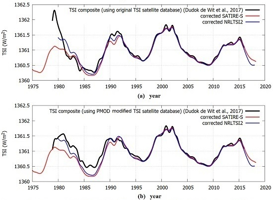
More recently, Dudok de Wit et al. [28] questioned whether the original satellite measured TSI database or the PMOD modified version should be used. They could not solve the problem and provided two preliminary versions of the TSI composite dependent on decisions about the data uncertainty: see Figure 4. In the following, we will propose a model test that uses the ACRIM1 records and the TSI composites by Dudok de Wit et al. [28] after the ACRIM-gap. Therefore, the controversial TSI records during the ACRIM-gap will be ignored as explained in the next sections.

Scafetta and Willson [42] had some critiques of the Dudok de Wit et al. work [28]. For example, it contains erroneous claims that ERBS/ERBE was the “only instrument observing during” the ACRIM-gap period while also showing the Nimbus7/ERB results in their Figure 1. They advocated for PMOD by claiming that there is “a growing consensus that Fröhlich’s corrections are a justifiable improvement to the original data”, ignoring the critical analyses of the original experimental teams that indicate otherwise [26,38,47] and providing no analytical alternatives. Dudok de Wit et al. [28] erroneously claimed their TSI composites better agree with PMOD than with ACRIM. In fact, this has been found not to be the case [42], as Figure 4 demonstrates since both TSI composites show an increase between 1986 and 1996.

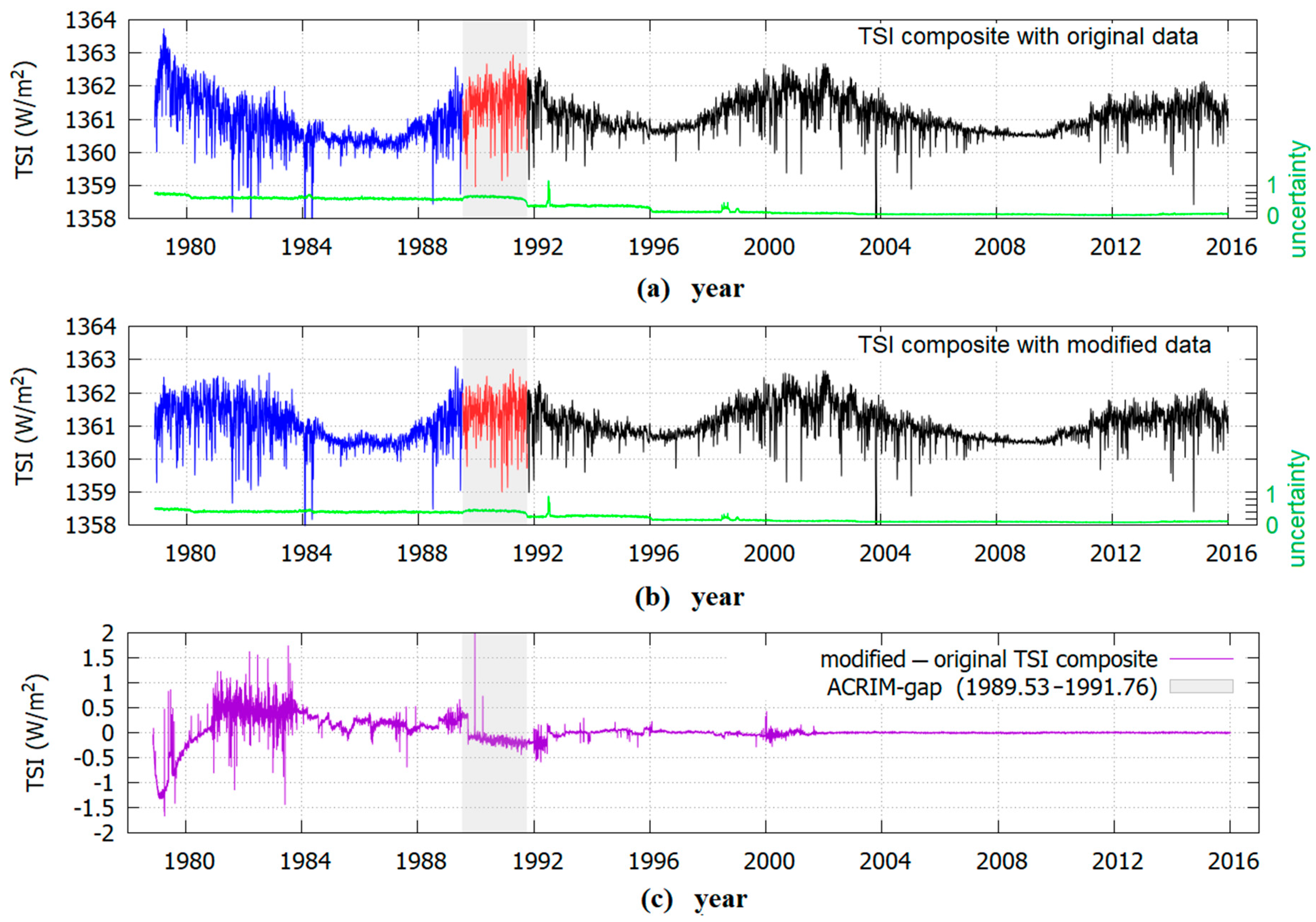
Finally, Dudok de Wit et al. [28] claimed that their TSI composites are affected by such large uncertainties (up to σ = 0.7 W/m² using the original TSI dataset, see Figure 4a, and up to σ = 0.4 W/m² using the modified TSI dataset, see Figure 4b) that it is impossible to discriminate between them or between the ACRIM and PMOD TSI records since 1981. Consequently, it would also be impossible to evaluate the TSI proxy models’ ability to reconstruct the quiet solar luminosity variability. However, a similar uncertainty issue was first noted and discussed in Scafetta [50] where it was determined that a large uncertainty curve originates when the cross-calibration of the TSI records uses very short overlapping intervals, like that used in the wavelet methodology by Dudok de Wit et al. [28]. Scafetta [50] determined the maximum possible composite uncertainty, which occurs using a point-to-point comparison of the various TSI datasets and obtained a similar, although slightly larger uncertainty curve. When all overlapping data are used at once, and one distinguishes between Nimbus7/ERB and ERBS/ERBE, the statistical uncertainty of the composites is greatly reduced because it scales with the root of the number of overlapping points [37]. Moreover, if we assume that the TSI uncertainty function evaluated in Dudok de Wit et al. [28] is meaningful, the comparison between their two proposed TSI composites should be made using some moving average smooth curve of the provided daily TSI records and the uncertainty range decreases with the root of the window size of the smoothing algorithm. For example, because the data have a daily resolution, the uncertainty associated with a 1–2 year moving average smooth curve (the statistical model proposed later by us will have approximately this resolution) would be about 20–27 times smaller than the daily uncertainty. Consequently, using a 1–2 year smoothed curve the uncertainty will be less than 0.035–0.025 W/m². This value is significantly smaller than the difference between the two TSI composites by Dudok de Wit et al. [28] (see

Table 1. TSI annual mean values in the 1986, 1996 and 2008 solar cycle minima and relative differences according to ACRIM, PMOD and the two TSI satellite composites proposed by Dudok de Wit et al. [28] using the original and the modified TSI satellite database.

TSI	Mean 1986 (W/m2)	Mean 1996 (W/m2)	Mean 2008 (W/m2)	Diff. 1996–1986 (W/m2)	Diff. 2008–1996 (W/m2)
ACRIM	1360.62 ± 0.01	1361.08 ± 0.01	1360.81 ± 0.01	+0.46 ± 0.01	–0.27 ± 0.01
PMOD	1360.59 ± 0.01	1360.54 ± 0.01	1360.41 ± 0.01	–0.05 ± 0.01	–0.13 ± 0.01
Original	1360.32 ± 0.03	1360.66 ± 0.01	1360.56 ± 0.01	+0.34 ± 0.04	–0.10 ± 0.02
Modified	1360.52 ± 0.02	1360.68 ± 0.01	1360.56 ± 0.01	+0.16 ± 0.03	–0.12 ± 0.02

) and it is up to 15–20 times smaller than the difference between ACRIM and PMOD TSI records from the TSI cycle minima in 1986 and 1996 (that is 0.45 + 0.08 = 0.53 W/m²). When these considerations are taken into account, the two TSI composites by Dudok de Wit et al. [28], as well as those proposed by ACRIM and PMOD are clearly distinguishable within their statistical uncertainty. Consequently, the various proposed solar models can be tested and evaluated against the data.

Dudok de Wit et al. [28] also noted that the variation functions among ACRIM3, VIRGO and SORCE-TIM from 2003–2013 appear equivalent to a 1/f red noise. Red noises are auto-regressive cumulative noises with long-range correlations. This result is likely due to the slight different sensitivity of the three experimental sensors [30]. It is difficult to assess which TSI record among the three better reproduced TSI data sets. However, it should be pointed out that VIRGO appears to be the most uncertain record because its main sensor (PMO6V-A) experienced an exceptionally large degradation of about 6 W/m² (nearly 4500 ppm) from 1996 to 2014, which has been corrected as discussed above [44]. VIRGO also experienced other satellite problems such as a failure of the PMO6V shutters at launch, which is responsible for their excessive degradation [26] (supplement). Both ACRIM3 and SORCE-TIM main sensors’ shutters worked properly and degraded much less by about 1000 and 200 ppm, respectively throughout their missions and therefore had self-calibration capabilities in space far more accurate than VIRGO’s [30,34]. The SORCE-TIM TSI record appears to have the least variability on the shortest observational timescales of the three experiments. This is most evident during the solar cycle minimum during 2008–2009: see Figure 2 [30] (Figure 4 and Figure 5). This is likely caused by the lower sensitivity of the TIM sensor. Between 2013 and 2014 SORCE-TIM also suffered a serious battery shutdown and failure that lasted about 7 months. Since 2003, both ACRIM3 and VIRGO show a more pronounced down-trending than SORCE-TIM [30]. The above considerations imply that among the three experiments ACRIM3 may better reproduce TSI variation until the first months of 2013.

While it is possible that any TSI measurements may be inaccurate because of some sensitivity issues, this possibility cannot be used to address the ACRIM-gap problem since we can only use ACRIM1 and ACRIM2 records. These two records do not overlap and, therefore, it is not possible to assess whether they deviate from each other according to a 1/f noise or anything else. Only random uncertainties can be assumed. On the contrary, any persistent bias between them and the proxy models needs to be ascribed to the inability of the latter to adequately reconstruct TSI variability in general, in particular during and around solar maxima [48]. In fact, proxy models frequently have significant differences from each as well. The challenge would be to find a way to reach a result convergence, as we will show below.

3. TSI Data and Models

We used the following observational TSI records: (1) ACRIM1 satellite TSI data [26,29] and (2) the recent TSI composites by Dudok de Wit et al. [28]. We compared them against the following TSI proxy records: (1) the recent TSI model proposed by Gueymard [24]; (2) the latest update of the SATIRE-S TSI model [16] and (3) the latest update of the NRLTSI2 model [15].

3.1. TSI Observations

The two TSI composites proposed by Dudok de Wit et al. [28] are herein adopted in place of the individual TSI satellite records produced by different science teams and their proposed TSI composites. This choice avoids a possible bias favoring a specific science group and its TSI products above the others. In fact, in reconstructing its TSI composites, ACRIM makes a preference for its own ACRIM1-2-3 satellite TSI records [30] while PMOD adopts its own VIRGO record since 1996 [33]. On the contrary, Dudok de Wit et al. [28] used time-varying weightings of all the available instrumental data whose uncertainties are also estimated in a systematic way yielding probably to a less-biased statistical approach for selecting instrumental weightings.

These authors proposed two TSI composites: one (Figure 4a) made with the original TSI database and the other (Figure 4b) with a database modified according to PMOD’s claims that some TSI satellite records need to be “corrected” in various different ways [27,35,40,41]. The two composites are nearly identical since 1992.5, as shown by their difference depicted in Figure 4c. They differ slightly from 1991.67 to 1992.5 because during this period PMOD modified the ACRIM2 record for a presumed uncorrected degradation, as described in Fröhlich (2004), which is disputed by ACRIM (see Appendix A). Finally, they differ significantly from 1978 to 1991.67 due to the heavy modifications implemented by PMOD to the Nimbus7/ERB record and to the ACRIM1 TSI satellite records from 1980 to 1984, as discussed in the Introduction.

Table 1 reports the TSI annual mean values during the 1986, 1996 and 2008 solar minima using the two proposed TSI composites by Dudok de Wit et al. [28]. As the table also reports, both TSI composites show a TSI increase between the TSI solar cycle minima in 1986 and 1996 (+0.34 ± 0.04 W/m² and +0.16 ± 0.03 W/m², respectively), and a slight decrease between the TSI solar cycle minima in 1996 and 2008 (–0.10 ± 0.02 W/m² and –0.12 ± 0.02 W/m², respectively).

As explained in the Introduction, some portions of the TSI satellite records are controversial. Thus, we made the choice to use in our following statistical algorithm only the likely most reliable TSI records in the following way:

(1) we used only the post ACRIM-gap portion of the TSI composites by Dudok de Wit et al. [28], which covered the period from 1991.76 to 2016;

(2) we ignored the Nimbus7/ERB record, which included the ACRIM-gap period and its contribution to TSI composite before 1989.53;

(3) We only used the ACRIM1 record after 1984.4 because from 1981 to 1984 ACRIM1 was affected by additional spin-mode solar pointing uncertainty caused by the failure of the precise solar pointing capability of the solar maximum mission satellite. In any case, despite this additional uncertainty during 1981–1984, ACRIM1 data are likely more reliable on the long scale than Nimbus7/ERB [26,29]. On the contrary, during the 1980–1984 period PMOD adopts a combination of Nimbus7/ERB and ACRIM1 records after modifying them with an empirical degradation model whose uncertainties are difficult to ascertain [27,41], see Figure 3.

Thus, the cross-scaling procedure proposed below in Section 4 used only the original ACRIM1 TSI record from 1984.4 to 1989.53 and the TSI composites by Dudok de Wit et al. [28] from 1991.76 to 2016, as depicted in the black curve of Figure 4a,b. The 1980–1981 ACRIM1 data did not have any known issue but it could not be included in the following analysis because it was relatively short and isolated.

3.2. TSI Proxy Models

Several daily resolution TSI models were proposed using alternative methodologies. The three TSI proxy models used in this study are shown in Figure 5.

Gueymard [24] proposed a TSI proxy model over the period 1976–2018 based on a non-linear combination of the daily sunspot number record, the daily radio flux at 10.7 cm (F107) record and the daily MgII index record, regressed against ACRIM, PMOD and SORCE-TIM records. Gueymard [24] also proposed a TSI composite, which can be downloaded from the journal website. His TSI composite should not be mistaken for his TSI proxy model, which is what we need to test (Gueymard, personal communication, June, 25, 2018). Gueymard’s TSI composite mostly uses the PMOD TSI record that, as explained, is made of modified TSI satellite data. Gueymard constructed his composite using his proxy model as a guide to cross-calibrate consecutive periods from 1976 to 2017 and to fill TSI missing daily data. In particular, from 1st October 1989 to 6^th March 2003 he only used PMOD (see his

Table 2. Linear scaling values of the scatter-plots depicted in Figure 6.

TSI Proxy	TSI-1 1981–1996	TSI-1 1996–2016	TSI-2 1981–1996	TSI-2 1996–2016
Gueymard	0.43 ± 0.01	0.66 ± 0.01	0.53 ± 0.01	0.67 ± 0.01
SATIRE-S	0.69 ± 0.01	0.92 ± 0.01	0.79 ± 0.01	0.93 ± 0.01
NRLTSI2	0.84 ± 0.01	0.96 ± 0.01	1.01 ± 0.01	0.97 ± 0.01

). This interval covers the controversial ACRIM-gap period too. Gueymard [24] justified his choice because his proxy model appeared more consistent with the PMOD lack of solar cycle minimum-to-minimum trending. However, this result could be explained by the fact that the TSI data modifications implemented by PMOD were originally guided by a TSI proxy model [35,40] similar to that adopted by Gueymard [24]. The problem is that Gueymard’s chosen TSI constructors, as well as those used in Fröhlich and Lean [35,40], do not show any significant solar cycle minimum-to-minimum trending because they are indicative of the solar active regions alone. Thus, by construction, those proxies cannot reproduce the solar cycle minimum-to-minimum trending of the ACRIM TSI composite and, therefore, they cannot be used to test whether such a trending exists or not.

Yeo et al. [16] proposed a SATIRE-S TSI model spanning from 1974 to 2013 based on full-disc observations from the KPVT, SoHO/MDI and SDO/HMI. This model ascribes variation in solar irradiance on timescales greater than a day to photospheric magnetism. This record can be considered as a semi-empirical model although herein we did not make any difference between semi-empirical and proxy models because in both cases they did not qualify as direct TSI measurements. We used an update of this model to 2018. Data available from http://www2.mps.mpg.de/projects/sun-climate/data/SATIRE-S_TSI_20180328.txt.

Coddington et al. [15] proposed a NRLTSI2 proxy model constructed using facular brightening and sunspot darkening features where the magnitude of the changes in TSI was determined from a linear regression of a proxy magnesium II (MgII) index and the sunspot area index against the approximately decade-long solar irradiance measurements of the solar radiation and climate experiment (SORCE). This TSI proxy model is an evolution of the model used in Fröhlich and Lean [35,40] to modify TSI experimental records. This model uses as constructors observables mostly indicative of the solar active regions alone as constructors and, therefore, cannot detect any significant change occurring in the quiet solar luminosity curve, as already explained above. We used an update of this model spanning from 1980 to 2018. Data available from https://catalog.data.gov/dataset/noaa-climate-data-record-cdr-of-total-solar-irradiance-tsi-nrltsi-version-2.

3.3. Direct Data Comparison

A common feature of the three TSI proxy models depicted in Figure 5 is that they show a very small to a slight decrease in the minimum-to-minimum TSI variability among the solar cycles 22 and 24 that occurred on September 1986, August 1996 and December 2008. Even assuming a ±0.2 W/m² uncertainty in their daily values [15], the uncertainty of the difference between two annual averages would be only ±0.015 W/m². Thus, the observed decadal trends in these TSI proxy models suggest that the TSI contribution from the quiet sun remained nearly constant or had slightly decreased during the last 40 years. This pattern more closely correlated with the multi-decadal trending shown by the PMOD TSI composite than with that of the ACRIM TSI composite. However, this 40-year downward trending appeared contradicted by the TSI solar cycle minimum-to-minimum trending shown by the two TSI composites proposed by Dudok de Wit et al. [28], as estimated above.

Differences between the TSI composites and the proxy models vary with time. Figure 6 compares smooth curves (based on a natural smoothing spline algorithm) of the two TSI composites proposed by Dudok de Wit et al. [28] and of the original SATIRE-S and NRLTSI2 TSI proxy models. Figure 6 highlights that the TSI composites and the proxy models agreed well for the period 1996–2016. However, they diverged significantly (by ~0.15 to ~0.7 W/m²) for the early period 1981–1996. This divergence was stronger for the SATIRE model. The TSI composite values for the period 1978–1981 could be disregarded because they were likely affected by a strong and uncorrected degradation of Nimbus7/ERB, which it was experiencing for the first time the high UV radiation of a solar cycle maximum [27,41].

The TSI observation-model differences were largely due to a scaling error that varied significantly between the early and later periods. Figure 7 compared scatter-plots between the two TSI composites by Dudok de Wit et al. [28] (right and left panels) and the three TSI proxy models in the periods 1981–1996 (red) and 1996–2016 (blue). Table 2 reports the various scaling factors.

The TSI proxy model proposed by Gueymard [24] shows a strong non-linear behavior versus the TSI composites, suggesting some limitations of the proxy model. Both SATIRE-S and NRLTSI2 model show a good linear behavior for the period 1996–2016 but for the period 1981–1996 a different scaling appeared together with some non-linearity. The most noticeable discrepancy in the TSI composites and the proxy models was the different scatter-plot slopes between the 1981–1996 and 1996–2016 periods. This slope divergence, or scaling error, was particularly evident for SATIRE-S.

NRLTSI2 appeared to perform better when compared against the second TSI composite by Dudok de Wit et al. [28] using the PMOD modified TSI database. However, this good behavior was likely due to mutual-calibration issues. In fact, NRLTSI2 was carefully calibrated against the SORCE/TIM (2003–present) TSI record [15] and, simultaneously, the PMOD modifications of the original TSI database before 2000 used in the second TSI composite were partially justified by a TSI proxy model using the same constructors of NRLTSI2 [35,40].

Due to these scaling and non-linearity errors, these proxy models could not accurately represent the original TSI observations. Even in the case of SATIRE-S and NRLTSI2, where their calibrations were made using TSI data from the period 1996–2016 (solar cycles 23 and 24), the scaling error yielded a poor reconstruction for the previous solar cycle 22 or the period 1981–1996.

4. Methods

Here we proposed to solve the differences highlighted in Table 1 and Table 2 by modeling the discrepancy between the TSI observation and the TSI proxy models using a polynomial regression function plus a Heaviside step function during the ACRIM-gap. The latter is necessary to optimally cross-calibrate the ACRIM1 record relative to the post ACRIM-gap TSI composite by Dudok de Wit et al. [28].

To bridge the nearly two-year ACRIM-gap period, the order of the polynomial function was chosen to be 17 since the regression period from 1984 to 2016 was 32 years long and a 2-year time resolution would be captured by a polynomial function with an order of 32/2+1 = 17, which had 17 nodes. The adoption of this order gives to the fitting function sufficient flexibility to capture the required 2-year time-scale variability while preventing any over-fitting. Thus, the model was made as:

$$f\left(t\right)={\displaystyle \sum }_{i=0}^{17}{a}_i{\left(t-2000\right)}^i+bH\left(1990.645-t\right)$$

(1)

where the variable “t” is measured in calendar year and 1990.645 and 2000 are calendar year dates. The Heaviside step function H(1990.645-t) is 1 for t < 1990.645 and 0 for t > 1990.645 and a₀, …, a₁₇ and b are the regression coefficients. The step date 1990.645 falls in the middle of the ACRIM-gap period, but this date can be substituted within the gap without altering the final result.

We used the nonlinear least-squares Marquardt–Levenberg algorithm to fit, using Equation (1), the residual records obtained by the difference between the TSI observations and the TSI proxy model predictions according to the equation:

$$TS{I}_{res}\left(t\right)=TS{I}_{obs}\left(t\right)-TS{I}_{mod}\left(t\right)$$

(2)

The fit precision limit was chosen to be 10⁻¹⁰.

The TSI mean value of the 1986 solar minimum in the original scale of the ACRIM1 record was 1367.01 W/m² (see Figure 2) [29], while the TSI mean value of the solar minimum of the year 1996 in the Dudok de Wit et al. [28] record was 1360.66 W/m²: the difference was 6.35 W/m². Thus, for visual and computational convenience we shifted the original TSI ACRIM1 record (http://www.acrim.com/) by 6.35 W/m² to align its 1986 solar cycle minimum with the 1996 one of the TSI composite of Dudok de Wit et al. [28]. This ACRIM1-Dudok de Wit combined record would constitute our TSI_obs(t). With this choice, the step function fit parameter b measured how much the ACRIM1 record must be shifted downward (if b > 0) to cross-calibrate it with the post 1991.76 TSI composite by Dudok de Wit et al. [28]. The polynomial function models the variation between the TSI observation and the TSI proxy model. Finally, the proxy model, TSI_mod(t), was empirically adjusted to optimally reproduce the data pattern within the chosen two-year timescale as the function TSI_corr(t), which is given by:

$$TS{I}_{corr}\left(t\right)=TS{I}_{mod}\left(t\right)+{\displaystyle \sum }_{i=0}^{17}{a}_i{\left(t-2000\right)}^i+bH\left(t-1990.645\right)$$

(3)

Note that the Heaviside step function has been inverted to simulate the evaluated scaling between ACRIM1 and the post ACRIM-gap TSI record.

We noted that the proposed methodology may be affected by boundary artifacts. However, they would be more pronounced before 1985 and after 2015 because these limits were open. However, the ACRIM-gap was bounded at both extremes. This period covered about 2 years, which is the resolution of the polynomial fit; this situation should greatly reduce the possible uncertainty of the model. In any case, in Section 5.3 we evaluated the statistical error of the fitting parameter b due to the 2-year data-gap using a Monte Carlo strategy.

5. Results

5.1. Using the TSI Composite Made of the Original Satellite Database

The TSI_res(t) functions referring to the three proxy models are shown in Figure 8. The TSI proxy model proposed by Gueymard [24] seriously underestimates the TSI solar cycle maximum 23 (1999–2003). The SATIRE-S [16] presents a significant downward trend relative to the observations, which is most evident from 1984 to 2000. The NRLTSI2 [15] presents an upward trend between 2005 and 2016. All three TSI proxy models have difficulty in properly simulate the TSI maxima, as Pap et al. [48] had already noted with earlier TSI proxy models regarding solar cycles 21 and 22. In particular, the three TSI proxy models herein analyzed underestimated the TSI rise observed in the ACRIM1 record from 1988 to 1989.53. The latter finding implies that the solar cycle minimum in 1986 was lower than what these proxy models predicted.

Regarding solar cycle 22, the regression model gives: b = 1.01 ± 0.14 W/m² using Gueymard [24]; b = 0.45 ± 0.06 W/m² using SATIRE and b = 0.38 ± 0.07 W/m² using NRLTSI2. Thus, TSI should have increased by ~0.4 W/m² from 1986 to 1996. For example, Figure 8 shows that these TSI proxy models underestimated the TSI rise occurred from 1987.5 to 1989.5 and slightly overestimated the TSI decrease from 1991.75 to 1994. The result was compatible with the cross-calibration between ACRIM1 and ACRIM2 TSI satellite record shown in the ACRIM TSI composite [38], which shows a 0.46 W/m² increase between these two TSI minima. Simultaneously, the same results contradicted the downward trend of the PMOD TSI composite between the two solar cycle minima from 1986 to 1996 (cf. Figure 3).

Figure 9 shows the three TSI proxy models after their modulation was corrected using Equation (3) from 1984.4 to 2016. The periods before 1984.9 and after 2015.5 were added without any modification but a simple cross-calibration based on the TSI means during the periods 1984.9–1985.4 and 2015.0–2015.5 for continuity. The three records, in particular, those depicted in the panels B and C, show a TSI solar minimum-to-minimum trending similar to the ACRIM TSI composite depicted in Figure 3.

5.2. Using the TSI Composite Made of the PMOD Modified Satellite Database

The calculations are now repeated using the second TSI composite of Dudok de Wit et al. [28] made using the TSI database modified with the PMOD correction hypotheses [27,35,40,41]. Figure 4b shows that from 1992.5 to 2016 this composite varies very little from the original one, but in the period from 1991.76 to 1992.5 is shifted down by ~0.2 W/m² mostly because of the PMOD modifications of the ACRIM2 record.

Figure 10 shows the analogous of Figure 8. We get: b = 1.54 ± 0.14 W/m² using Gueymard [24]; b = 0.98 ± 0.06 W/m² using SATIRE and b = 0.91 ± 0.07 W/m² using NRLTSI2. In this case, the TSI proxy models significantly underestimated the TSI rise from 1987.5 to 1989.5 and overestimated the TSI decrease from 1991.75 to 1994. Thus, we found a larger difference between the TSI composite made with the modified TSI database and the proxy models. In this case, the TSI rise between the solar cycle minima in 1986 and 1996 should be significantly greater than in the previous case. SATIRE and NRLTSI2 again appeared to perform better than the TSI model by Gueymard [24].

5.3. Evaluation of the Statistical Uncertainty of the Model

The significance of the above results should be evaluated against the null hypothesis that the residual function TSI_res(t), Equation (2), is made of Gaussian noise. In such an eventuality, the regression coefficient of Equation (1), a₀, a₁, …, a₁₇ were expected to be equal to 0 ± σ_i (for i = 0, 1, …, 17) while b was expected to be equal to 0 ± σ_b. The main issue was to evaluate whether the regression parameters b evaluated in Section 5.1 and Section 5.2, which measured the step size between the TSI cycle minima in 1986 and 1996, was significantly larger than its theoretical statistical error σ_b. In other words, we would like to determine whether the evaluated parameter b was positive despite its estimated error.

This was done using a Monte Carlo approach. A set of synthetic sequences of normalized Gaussian noise (σ_g = 1) as long as the data (10732 data) and showing the same ACRIM-gap period were generated. Equation (1) was applied to them to find that σ_b = 0.47 σ_g.

The standard deviation σ for the three TSI_res(t) records shown in Figure 8 was σ = 0.31 W/m², σ = 0.19 W/m² and σ = 0.17 W/m², respectively. These estimated uncertainties were compatible with the reported 20% uncertainty relative to the 11-year solar cycle amplitude of the facular and sunspot proxy indices [15] but appeared higher than the claimed 4% uncertainties of the pixel averaged magnetic flux density (<Bl>/μ) used in the SATIRE model [16]. Thus, the error associated to our model was about σ_b = 0.15 W/m², σ_b = 0.09 W/m² and σ_b = 0.08 W/m² for Gueymard [24], SATIRE and NRLTSI2, respectively.

By combining the fitting error of b estimated in Section 5.1 and Section 5.2 with σ_b, for the two TSI composite cases we got: b = 1.01 ± 0.2 W/m² and b = 1.54 ± 0.2 W/m² (using Gueymard [24]); b = 0.45 ± 0.1 W/m² and b = 0.98 ± 0.1 W/m² (using SATIRE-S) and b = 0.38 ± 0.1 W/m² and b = 0.91 ± 0.1 W/m² (using NRLTSI2). These values are listed also in

Table 3. Values of the step function parameter b used for the modified TSI models depicted in Figure 9, Figure 11 and Figure 12.

	Gueymard W/m2	SATIRE-S W/m2	NRLTSI2 W/m2
ACRIM1 and TSI-1	1.01 ± 0.2	0.45 ± 0.1	0.38 ± 0.1
ACRIM1 and TSI-2	1.54 ± 0.2	0.98 ± 0.1	0.91 ± 0.1

.

Since our values of b were more than three times larger than their statistical uncertainty σ, we concluded that they indicated that the TSI cycle minimum in 1986 was significantly below the TSI cycle minimum in 1996 by at least 0.4 ± 0.1 W/m² with a confidence larger than 99%.

The uncertainty between the TSI cycle minima in 1986 and 1996 estimated with our method (± 0.1 W/m²) was also significantly smaller than those estimated using the method by Dudok de Wit et al. [28]. From the TSI cycle minimum in 1996 to that in 1986, for the two TSI composites, the given uncertainty increased from 0.2 to 0.6 W/m² and 0.17 to 0.4 W/m², respectively.

6. Discussion

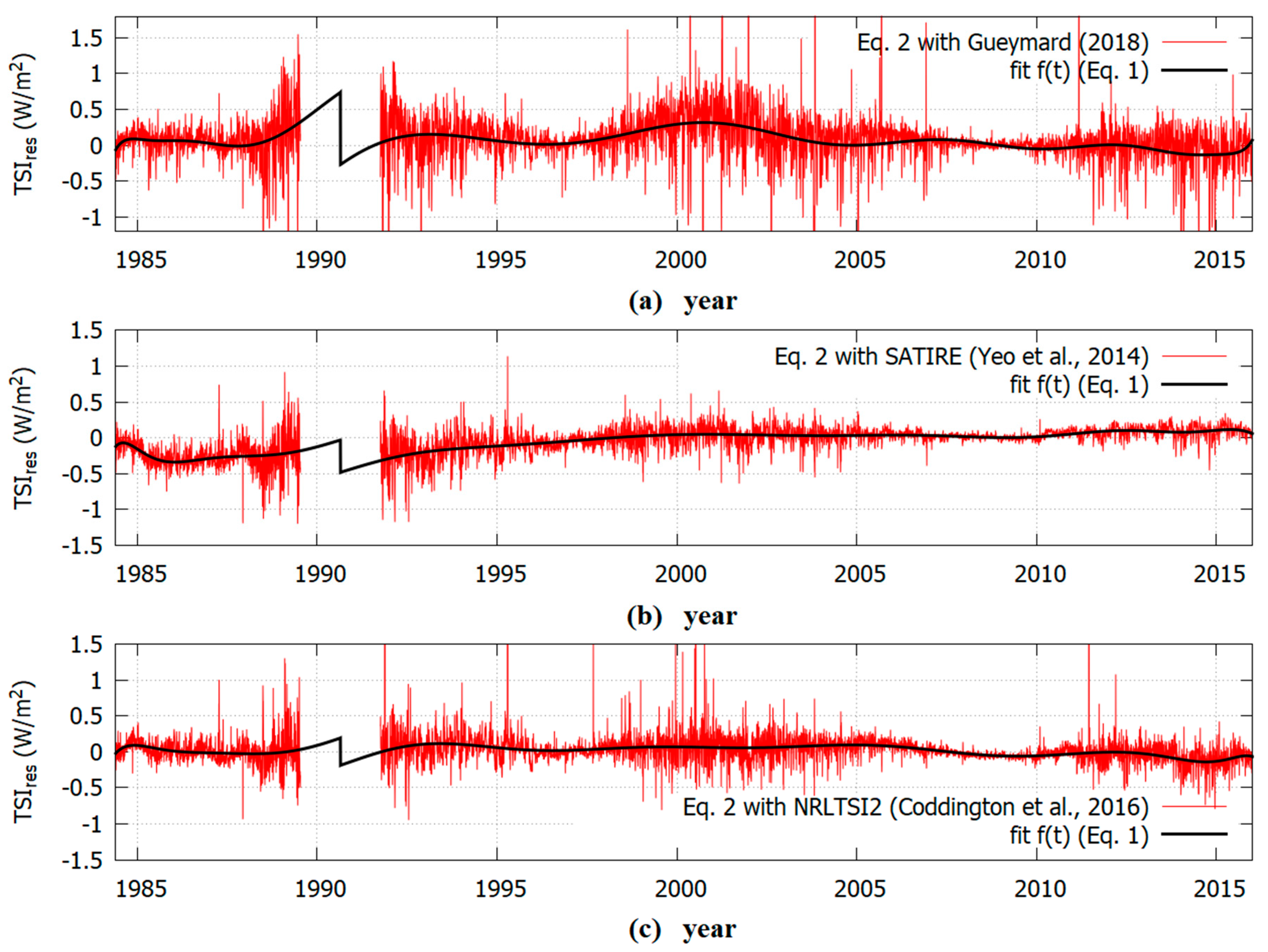
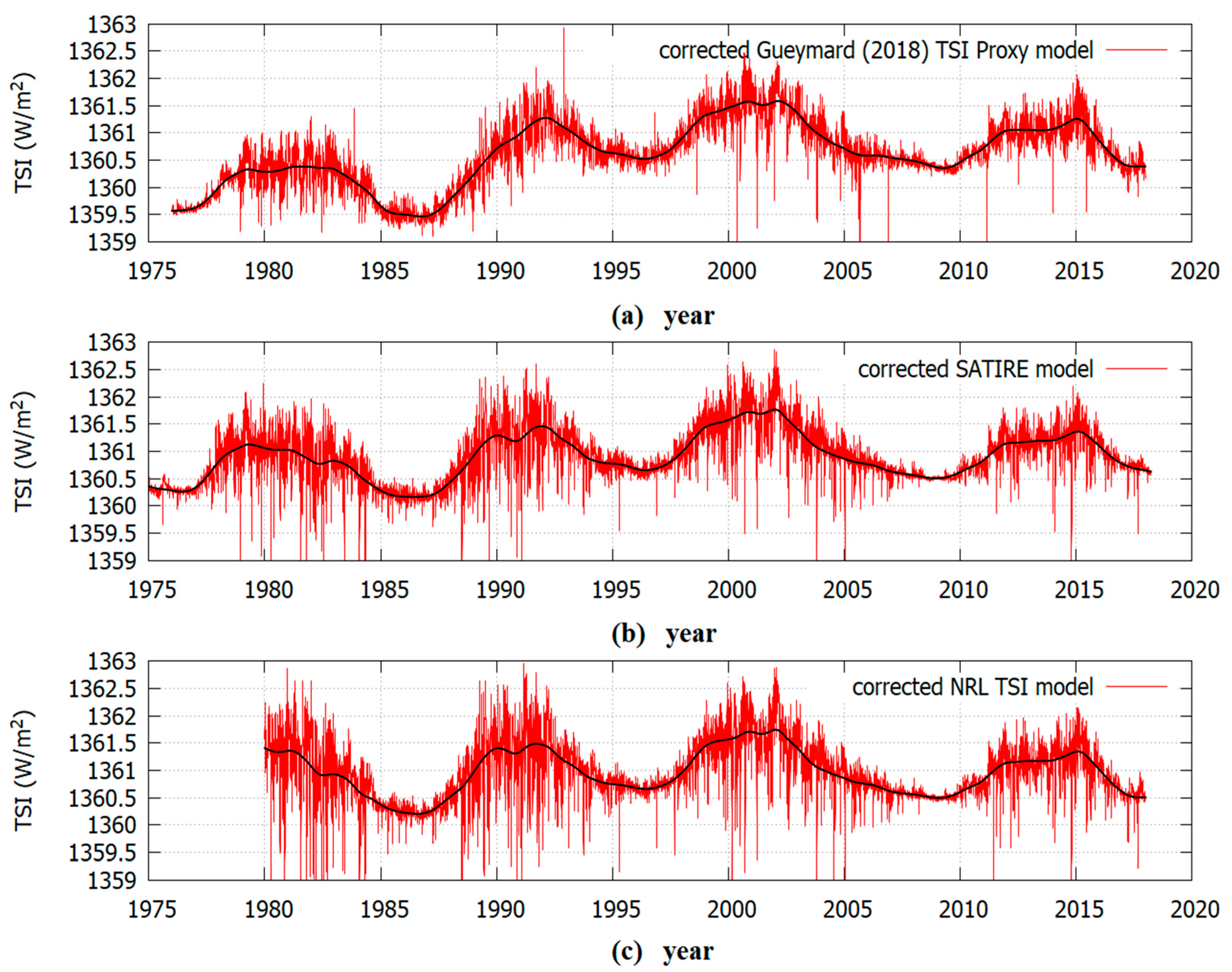
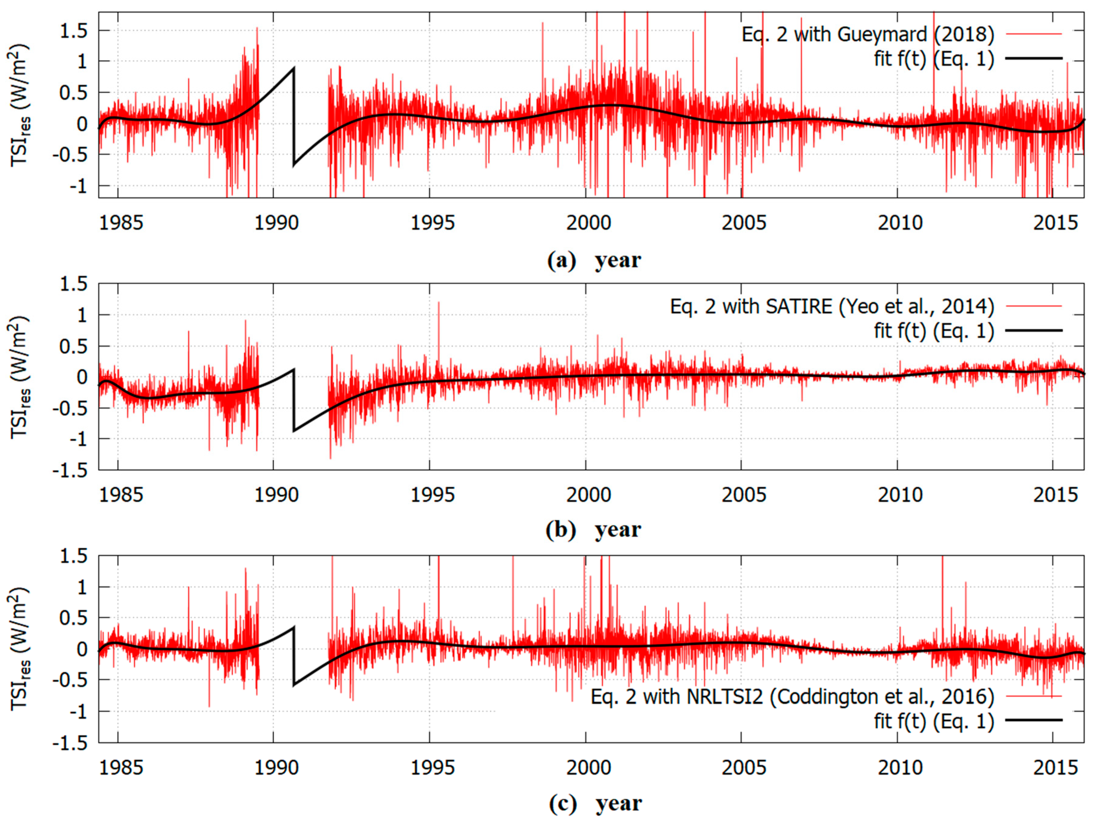
The above analysis suggests that the TSI proxy model proposed by Gueymard [24] was too unstable and, consequently, also the attempt to correct it using the regression methodology of Equation (1) could produce an unreliable result. On the contrary, the results obtained with the SATIRE and NRLTSI2 models were more consistent with each other.

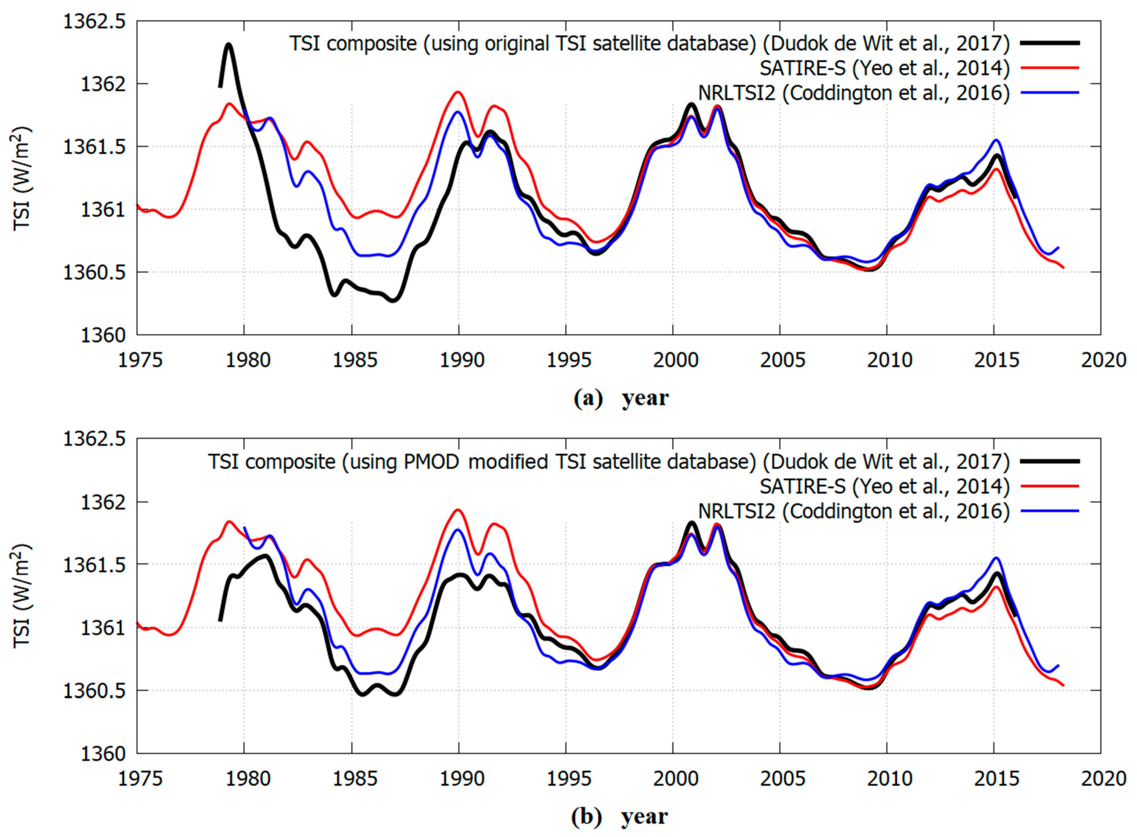
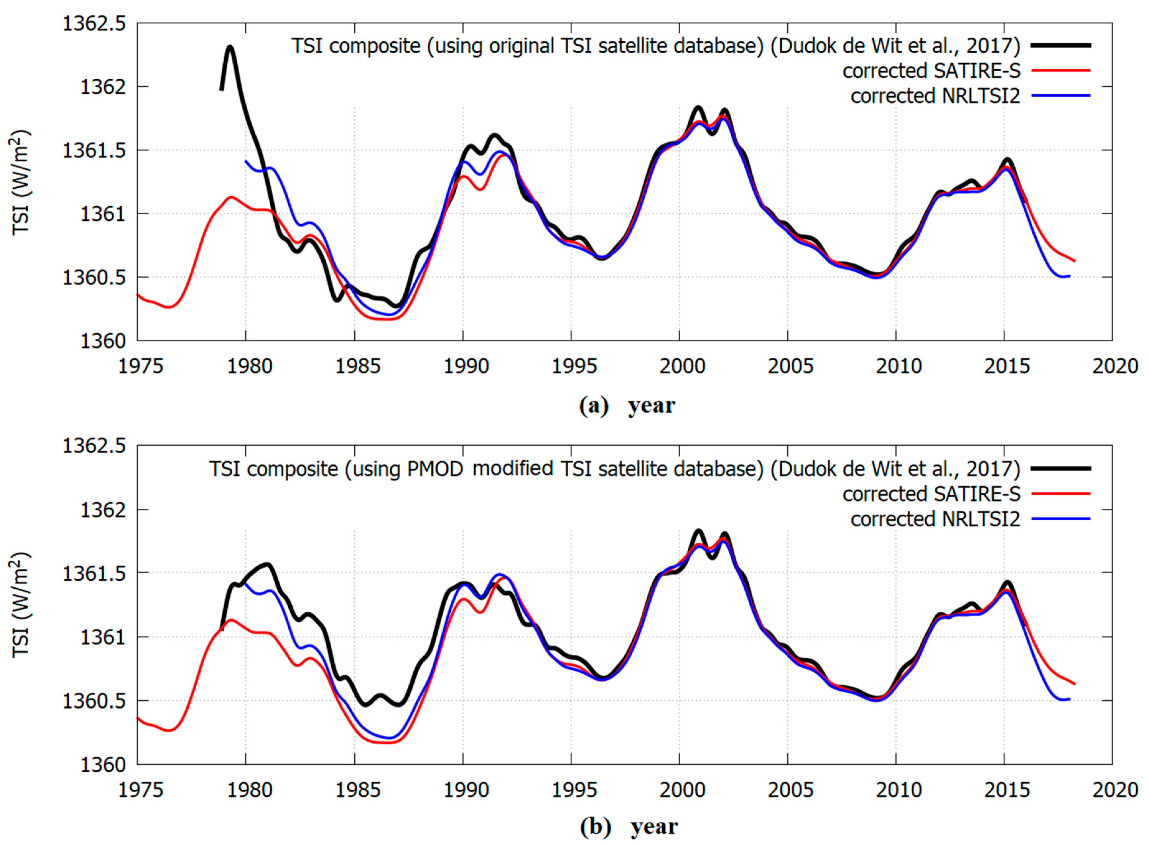
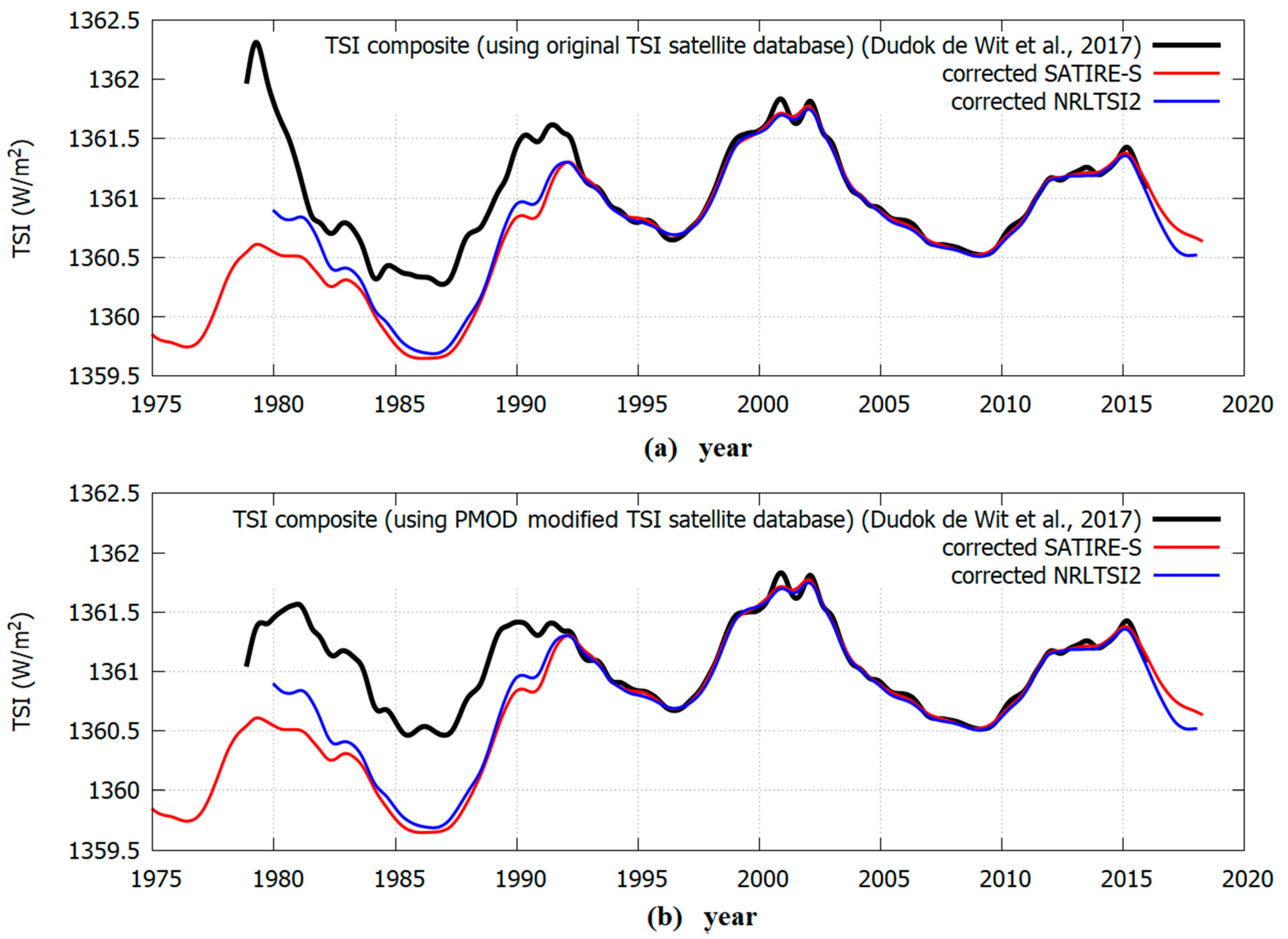
Figure 11 shows the modified SATIRE-S and NRLTSI2 TSI proxy models shown in Figure 9. It was observed that the two proxy models now agreed well with each other and with the TSI composite obtained using the original database within a 0.1 W/m² error for most of the overlapping period from 1981 to 2016: see Figure 11a. The significant discrepancy observed from 1978 to 1981 was caused by the uncorrected degradation of the Nimbus7/ERB record, as explained above.

A slightly better agreement for the period 1981–1992 between the modified TSI proxy model curves with the observations could possibly be obtained if the TSI composite would not use the ERBS/ERBE record, which was the one with the largest uncertainty and was affected by significant degradation from 1989 to 1992 during its first exposure to the high UV emissions during the maximum of the solar cycle 22. Not using the ERBS/ERBE record in the TSI composite should result in a slightly lower TSI minimum in 1986.

On the contrary, Figure 11b shows that there still persisted a significant discrepancy up to 0.3 W/m² with the TSI composite obtained using the PMOD’s modified TSI database. Thus, the evidence was that those modifications worsened the discrepancy with the proxy models and, therefore, they were likely incorrect.

Indeed, the good agreement between the two modified proxy models and the TSI composite from 1981 to 1992 using the original TSI database depicted in Figure 11a suggest that the result was consistent and robust. In fact, the SATIRE-S and the NRLTSI2 proxy models were independently constructed and the regression correction model proposed in Eqs. 1 and 2 did not use the TSI composite values prior to 1991.76.

Figure 12 is analogous to Figure 11 but now the TSI proxy models were modulated according to the results depicted in Figure 10 where the calibration used the second TSI composite by Dudok de Wit et al. [28] made with the PMOD modified TSI satellite database. The modified SATIRE-S and the NRLTSI2 proxy models were again highly correlated and show a TSI increase between the solar cycle minima in 1986 and 1996 of about 1 W/m². However, both models poorly correlated with both TSI composites by Dudok de Wit et al. [28] for the period 1980–1991.76.

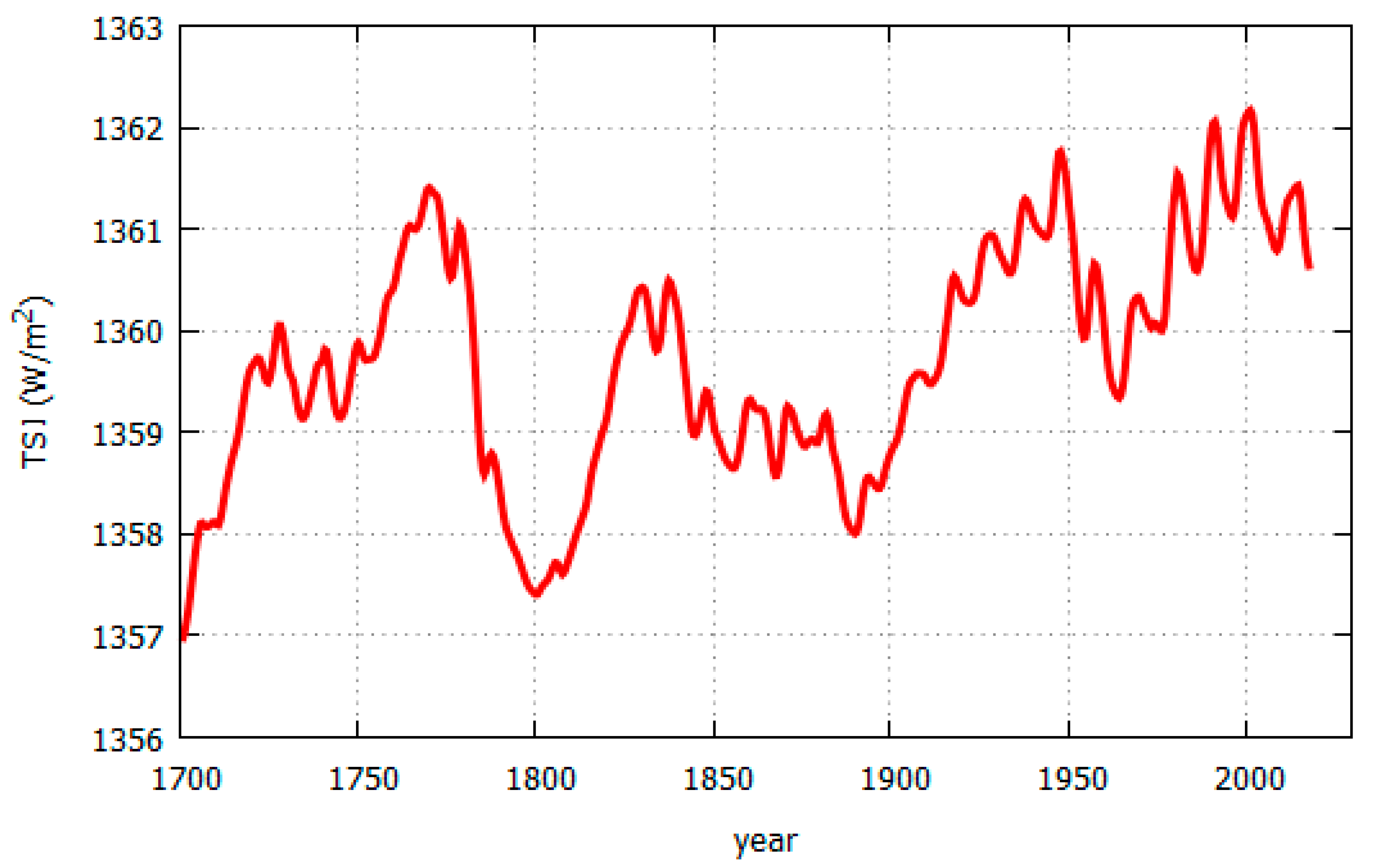
The modeled TSI pattern suggests that 2000–2002 could have been a grand solar maximum. Figure 13 shows a TSI evolutionary model that used the solar proxy model [1] that attempted to reconstruct the quiet solar luminosity variability based on Schwabe cycle length (rather than average solar cycle amplitude). This model was extended using the ACRIM composite since 1981 and an average between VIRGO and SORCE TIM since 2013. This particular TSI model appeared to correlate well with the Earth’s global surface temperature records since 1700 [1,20,21,51].

The TSI data from 1978 to 1981 appeared too corrupted because of uncorrected degradation of the Nimbus7/ERB sensors during the solar maximum of cycle 21. For this reason, it was more appropriate to dismiss the data from this period because modifying TSI data using proxy models, as done by PMOD, would be arbitrary. We proposed that any reliable TSI composite should begin from late 1980 with the ACRIM1 record.

The currently proposed TSI proxy models, such as SATIRE and NRLTSI2, appeared to be more reliable in reconstructing the fast fluctuations of TSI variability but failed to properly model longer low-frequency timescales. In particular, they were found to best agree with the TSI composites after 1996. However, a progressive divergence was observed for the early period (e.g., 1981–1996). This suggests that the relation between TSI and its used proxies was not stationary but varied in time. Probably their scaling errors also evolved in time. Due to the non-stationary uncertainties in the observations, these proxy models were likely missing a slowly varying TSI component that needed to be non-linearly coupled with the typical adopted solar proxies (SSN and SSA, MgII, F106, etc.), which were more indicative of the active solar regions. Therefore, there was a need to develop better quiet sun luminosity models as the proposed evidence indicates that TSI background levels may vary significantly from cycle to cycle.

An increase in solar activity from 1970 to 2000 is predicted by alternative solar theoretical models. One model predicting such a TSI increase between 1986 and 1996 was based on the negative correlation found between solar cycle length and solar and climate variability on century timescales [1,51,52]. This model predicted the recent TSI increase because solar cycle 22 (1986–1996) was 9.9-year long and was significantly shorter than the 11-year Schwabe solar cycle length mean and shorter than both solar cycle 21 (1976–1986, 10.5 year) and solar cycle 23 (1996–2008, 12.3 year). According to this model, the shortness of cycles 21 and 22 should have progressively stressed the solar dynamo and increased the quiet solar luminosity variability from the 1970s to 2000. During the maximum of solar cycle 22 this TSI behavior would be confirmed by the upward trending observed in the Nimbus7/ERB TSI record and in other solar magnetic activity records during the ACRIM-gap [38]. The decrease of solar activity observed since 2000 may have been caused by the solar dynamo slowdown of cycle 23 that would likely persist for solar cycle 24 as well. It should be noticed that a negative correlation was also found between the Earth’s global surface temperature and the Earth’s length of the day (LOD) record, suggesting a direct link between the surface temperature of a celestial body and overall circulation patterns of its atmosphere [53].

The multi-decadal to millennial solar activity oscillations could be interpreted and reconstructed by using also the astronomical resonances of the solar system. In fact, they appear to drive and synchronize the main solar oscillations [54,55,56]. More specifically, a TSI peak in the 1940s, its following decrease until around 1970 and again its increase from 1970 to 2000 and decrease afterward (cf. Figure 13) would be part of a 60-year oscillation. This is one of the typical oscillations commonly observed in climate ([20,21,57]; and references therein) and solar records [58,59,60] based on actual observations. Scafetta’s [54] harmonic solar model predicted several decadal to millennial solar and climate oscillations throughout the entire Holocene and even during the Marine Interglacial Stage 9.3 that occurred 325–336 kyear ago [56,61]. According to this interpretation, the 2000–2002 TSI peak was caused by the maximum of the gravitational pull of Jupiter and Saturn on the sun that reached its 60-year cycle maximum around 2000. This gravitational pull could have increased solar luminosity production by a tidal forcing [55]. Other interpretations involving an electromagnetic coupling between the sun and the planets may be also possible [62,63]. The same harmonic solar model suggests that the sun may now be heading toward a new grand solar minimum in the 2030–2040 time frame.

Final evidence that TSI may have increased from 1980 to 2000 comes from Earth’s climate studies. Secular climate records correlate well with TSI curves such as the one depicted in Figure 13 and on longer ones covering the entire Holocene [1,23,60,64]. In particular, the warming observed from 1970 to 2000, followed by a temperature standstill since 2000, is a good fit for a natural 60-year cycle prediction superimposed to other contributions [20]. This pattern correlates better with a TSI evolution similar to the ACRIM composite [17,18,19,20,21,62,65] than with the CMIP5 general circulation climate model predictions of continuous anthropogenic warming [22]. The CMIP5 climate models use a high climate sensitivity to CO₂ forcing and low secular TSI variability proxy models, such as the one proposed in [3], which was calibrated using the PMOD TSI composite model after 1980.

7. Conclusions

Herein we reviewed the ACRIM-PMOD controversy regarding whether TSI increased from 1980 to 2000 and proposed an alternative solution. Solving this issue is crucial to understand how the quiet solar luminosity varies and it is important for climate change studies. This controversy can be reduced to the issue of the appropriateness of modifying TSI observations using TSI proxy model predictions. Our finding was that the disagreements between TSI observations and proxy model predictions were primarily caused by flaws in the models, indicating that the relationships between solar physical models and TSI variability was not yet well-understood.

We noted that Pap et al. [48] came also to the conclusion that the disagreement between data and proxy models “seems to be more of a problem with the models than with the instruments”. Yet only a few years later, despite this finding, TSI proxy models were used to empirically “correct” TSI observations to produce the PMOD TSI composites [35,40]. The approach adopted by Fröhlich and Lean [35,40] involved no work with the original observational data or in-depth consultation with the TSI satellite experiment teams. Yet, the PMOD composite was favored by part of the scientific community [22,28] despite objections from the original TSI experiment teams who could find no experimental issues to justify the satellite data modifications proposed by Frohlich and Lean. See Willson and Mordvinov [26] and Hoyt’s statement in Scafetta and Willson [38] that is partially reproduced in Appendix A.

Here we reversed the PMOD approach. We used the uncontroversial TSI observations before and after the ACRIM-gap period (1989.53–1991.67) to empirically adjust the low-frequency component of the TSI proxy models in an attempt to bridge the gap. This approach explicitly allows the possibility that those proposed models could be missing a slow varying solar luminosity component of the quiet sun regions. In brief, we attempted to solve the ACRIM-gap problem by ignoring both Nimbus/ERBS and ERBS/ERBE, lower quality TSI records than ACRIM1 and ACRIM2, and evaluated how the modified proxy models reconstruct the rising and declining periods of solar cycle 22, just before and after the gap, respectively. Our statistical methodology modeled the biannual trending of the TSI record from 1978 to date and bridged the ACRIM-gap. Although the proposed regression methodology works best when the records do not have gaps, it may still be reliable for bridging minor gaps in the data by reconstructing its optimal geometry as suggested by the entire record.

We found that the models underestimated the TSI cycle 22 rising trend and overestimated the solar cycle 22 declining trend. Problems in properly reconstructing solar cycles 23 and 24 maxima were also observed. Such divergences have been typically observed and are likely due to solar effects not taken into account in the models [66]. After empirically adjusting the models for these biases, our best result appeared to be the one shown in Figure 11A where we found consistency between the adjusted proxy models and the TSI composite proposed by Dudok de Wit et al. [28] constructed with the unmodified TSI database since about 1981. This composite shows better agreement with the ACRIM composite than with PMOD.

Our method provides a new TSI data record showing TSI increased by at least 0.4 W/m² from the 1986 to the 1996 solar cycle minimum and twice as much from 1980 to 2002. It decreased since 2002 by ~0.15 W/m² from the 1996 to the 2009 solar cycle minimum. The ACRIM TSI composite shows a very similar pattern with a slightly larger increase of about 0.46 W/m² between 1996 and 2008 and a decrease of about 0.27 W/m² between 1996 and 2009. The PMOD TSI record shows an incompatible pattern with a slight decrease of ~0.05 W/m² from 1986 to 1996 followed by an additional decrease of ~0.13 W/m² between 1996 and 2009.

The above result was consistent with those already shown in Scafetta and Willson [38,47] using other TSI models. Scafetta and Willson [47] bridged the ACRIM-gap using the SATIRE-T model proposed by Krivova et al. [67], which was labeled KBS07 and showed that the resulting ACRIM-KBS07 and PMOD-KBS07 constructions confirmed the ACRIM composite trend. Krivova et al. [68] critiqued the result claiming that their SATIRE-T model was not supposed to accurately reconstruct TSI changes on the monthly time scales but only on the decadal-scale and above. However, Scafetta and Willson [38] showed that during the ACRIM-gap PMOD diverged also from the TSI models of Wenzler et al. [69] and Ball et al. [70]. Moreover, it was shown that the divergences between the SATIRE-T model and the data on a decadal time scale provided a confirmation of the trending shown by the ACRIM TSI composite. The SATIRE-S model was also analyzed and the result was still the same: the divergence between the data and the model confirmed a TSI upward trend during the ACRIM-gap and, therefore, the ACRIM TSI satellite composite trending. Thus, the claimed agreement between PMOD and several TSI models appeared coincidental because it seemed due simply to the inability of these models to properly reconstruct the quiet solar luminosity variability.

A reliable assessment of the quiet solar luminosity variation depends on continuous and accurately calibrated TSI measurements. The Total and Spectral Solar Irradiance Sensor-1 (TSIS-1) on the International Space Station began measuring TSI since 2018 to extend the 40 years of TSI observations. The Total Solar Irradiance Monitor (TSIM) onboard the Chinese Feng Yun-3C (FY-3C) satellite is also measuring TSI from space since 2013 [71,72]. The importance of the long term TSI measurement database cannot be overemphasized for understanding the TSI variability on decadal to millennial timescales in the past, to assess the TSI variability impact on climate change in the future.

References

1. Hoyt, D.V.; Schatten, K.H. A discussion of plausible solar irradiance variations, 1700–1992. J. Geophys. Res. 1993, 98, 895–906. [Google Scholar] [CrossRef]
2. Lean, J.; Beer, J.; Bradley, R. Reconstruction of solar irradiance since 1610: Implications for climate change. Geophys. Res. Lett. 1995, 22, 3195–3198. [Google Scholar] [CrossRef] [Green Version]
3. Wang, Y.-M.; Lean, J.L.; Sheeley, N.R.J. Modeling the Sun’s magnetic field and irradiance since 1713. Astrophys. J. 2005, 625, 522. [Google Scholar] [CrossRef]
4. Tapping, K.F.; Boteler, D.; Charbonneau, P.; Crouch AManson, A.; Paquette, H. Solar magnetic activity and total irradiance since the Maunder minimum. Sol. Phys. 2007, 246, 309–326. [Google Scholar] [CrossRef]
5. Steinhilber, F.; Beer, J.; Fröhlich, C. Total solar irradiance during the Holocene. Geophys. Res. Lett. 2009, 36, L19704. [Google Scholar] [CrossRef]
6. Krivova, N.A.; Vieira, L.E.A.; Solanki, S.K. Reconstruction of solar spectral irradiance since the Maunder minimum. J. Geophys. Res. 2010, 115, a12112. [Google Scholar] [CrossRef]
7. Vieira, L.E.A.; Solanki, S.K.; Krivova, N.A.; Usoskin, I. Evolution of the solar irradiance during the Holocene. A&A 2011, 531, A6. [Google Scholar] [Green Version]
8. Shapiro, A.I.; Schmutz, W.; Rozanov, E.; Schoell, M.; Haberreiter, M.; Shapiro, A.V.; Nyeki, S. A new approach to the long-term reconstruction of the solar irradiance leads to large historical solar forcing. A&A 2011, 529, A67. [Google Scholar] [Green Version]
9. Solanki, S.K.; Krivova, N.A.; Haigh, J.D. Solar irradiance variability and climate. Annu. Rev. Astron. Astrophys. 2013, 51, 311–351. [Google Scholar] [CrossRef]
10. Kopp, G. Magnitudes and timescales of total solar irradiance variability. J. Space Weather Space Clim. 2016, 6, A30. [Google Scholar] [CrossRef] [Green Version]
11. Matthes, K.; Funke, B.; Andersson, M.E.; Barnard, L.; Beer, J.; Charbonneau, P.; Clilverd, M.; Dudok de Wit, T.; Haberreiter, M.; Hendry, A.; et al. Solar forcing for CMIP6 (v3.2). Geosci. Model Dev. 2017, 10, 2247–2302. [Google Scholar] [CrossRef] [Green Version]
12. Egorova, T.; Schmutz, W.; Rozanov, E.; Shapiro, A.I.; Usoskin, I.; Beer, J.; Tagirov, R.V.; Pete, T. Revised historical solar irradiance forcing Revised historical solar irradiance forcing. A&A 2018, 615, A85. [Google Scholar]
13. Beer, J.; Tobias, S.; Weiss, N. An Active Sun Throughout the Maunder Minimum. Sol. Phys. 1998, 181, 237–249. [Google Scholar] [CrossRef] [Green Version]
14. Owens, M.J.; Usoskin, I.; Lockwood, M. Heliospheric modulation of galactic cosmic rays during grand solar minima: Past and future variations. Geophys. Res. Lett. 2012, 39, L19102. [Google Scholar] [CrossRef]
15. Coddington, O.; Lean, J.; Pilewskie, P.; Snow, M.; Lindholm, D. A solar irradiance climate data record. Bull. Am. Meteorol. Soc. 2016, 97, 1265–1282. [Google Scholar] [CrossRef]
16. Yeo, K.L.; Krivova, N.A.; Solanki, S.K.; Glassmeier, K.H. Reconstruction of total and spectral solar irradiance from 1974 to 2013 based on KPVT, SoHO/MDI and SDO/HMI observations. Astron. Astrophys. 2014, 570, A85. [Google Scholar] [CrossRef]
17. Scafetta, N.; West, B.J. Estimated solar contribution to the global surface warming using the ACRIM TSI satellite composite. Geophys. Res. Lett. 2005, 32, L18713. [Google Scholar] [CrossRef]
18. Scafetta, N.; West, B.J. Phenomenological solar signature in 400 years of reconstructed Northern Hemisphere temperature record. Geophys. Res. Lett. 2006, 33, L17718. [Google Scholar] [CrossRef]
19. Scafetta, N. Empirical analysis of the solar contribution to global mean air surface temperature change. Atmos. Sol. Terrest. Phys. 2009, 71, 1916–1923. [Google Scholar] [CrossRef] [Green Version]
20. Scafetta, N. Discussion on climate oscillations: CMIP5 general circulation models versus a semiempirical harmonic model based on astronomical cycles. Earth Sci. Rev. 2013, 126, 321–357. [Google Scholar] [CrossRef]
21. Scafetta, N. Solar and planetary oscillation control on climate change: Hind-cast, forecast and a comparison with the CMIP5 GCMS. Energy Environ. 2013, 24, 455–496. [Google Scholar] [CrossRef]
22. IPCC. Climate Change 2013: The Physical Science Basis. Contribution of Working Group I to the Fifth Assessment Report of the Intergovernmental Panel on Climate Change; Stocker, T.F., Qin, D., Plattner, G.-K., Tignor, M., Allen, S.K., Boschung, J., Nauels, A., Xia, Y., Bex, V., Midgley, P.M., Eds.; Cambridge University Press: Cambridge, UK; New York, NY, USA, 2013; p. 1535. [Google Scholar] [CrossRef]
23. Soon, W.; Connolly, R.; Connolly, M. Re-evaluating the role of solar variability on Northern Hemisphere temperature trends since the 19th century. Earth-Sci. Rev. 2015, 150, 409–452. [Google Scholar] [CrossRef]
24. Gueymard, C.A. A reevaluation of the solar constant based on a 42-year total solar irradiance time series and a reconciliation of spaceborne observations. Sol. Energy 2018, 168, 2–9. [Google Scholar] [CrossRef]
25. Foukal, P.A.; Lean, J.L. An empirical model of total solar irradiance variation between 1874 and 1988. Science 1990, 247, 556–558. [Google Scholar] [CrossRef]
26. Willson, R.C.; Mordvinov, A.V. Secular total solar irradiance trend during solar cycles 21–23. Geophys. Res. Lett. 2003, 30, 1199–1203. [Google Scholar] [CrossRef]
27. Fröhlich, C. Solar irradiance variability since 1978. Space Sci. Rev. 2006, 125, 53–65. [Google Scholar] [CrossRef]
28. Dudok de Wit, T.; Kopp, G.; Fröhlich, C.; Schöll, M. Methodology to create a new total solar irradiance record: Making a composite out of multiple data records. Geophys. Res. Lett. 2017, 44, 1196–1203. [Google Scholar] [CrossRef] [Green Version]
29. Willson, R.C. Total solar irradiance trend during solar cycles 21 and 22. Science 1997, 277, 1963–1965. [Google Scholar] [CrossRef]
30. Willson, R.C. ACRIMSAT/ACRIM3 update and the Total Solar Irradiance databases. Astrophys. Space Sci. 2014, 352, 341–352. [Google Scholar] [CrossRef]
31. Hoyt, D.V.; Kyle, H.L.; Hickey, J.R.; Maschhoff, R.H. The Nimbus 7 solar total irradiance: A new algorithm for its derivation. J. Geophys. Res. 1992, 97, 51–63. [Google Scholar] [CrossRef]
32. Lee, R.B., 3rd; Gibson, M.A.; Wilson, R.S.; Thomas, S. Long-term total solar irradiance variability during sunspot cycle 22. J. Geophys. Res. 1995, 100, 1667–1675. [Google Scholar] [CrossRef]
33. Fröhlich, C. Total solar irradiance observation. Surv. Geophys. 2012, 33, 453–473. [Google Scholar] [CrossRef]
34. Kopp, G. An assessment of the solar irradiance record for climate studies. J. Space Weather Space Clim. 2014, 4, A14. [Google Scholar] [CrossRef] [Green Version]
35. Fröhlich, C.; Lean, J. The Sun’s total irradiance: Cycles, trends and related climate change uncertainties since 1976. Geophys. Res. Lett. 1998, 25, 4377–4380. [Google Scholar] [CrossRef]
36. Dewitte, S.; Nevens, S. The total solar irradiance climate data record. Astroph. J. 2016, 830, 25. [Google Scholar] [CrossRef]
37. Scafetta, N. Total Solar Irradiance Satellite Composites and their Phenomenological Effect on Climate. In Evidence-Based Climate Science; Easterbrook, D., Ed.; Elsevier: Amsterdam, The Netherlands, 2011; Volume 12, pp. 289–316. [Google Scholar]
38. Scafetta, N.; Willson, R.C. ACRIM total solar irradiance satellite composite validation versus TSI proxy models. Astrophys. Space Sci. 2014, 350, 421–442. [Google Scholar] [CrossRef] [Green Version]
39. Chapman, G.A.; Cookson, A.M.; Dobias, J.J. Variations in total solar irradiance during solar cycle 22. J. Geophys. Res. 1996, 101, 13541–13548. [Google Scholar] [CrossRef]
40. Fröhlich, C.; Lean, J. Solar radiative output and its variability: Evidence and mechanisms. Astron. Astrophys. Rev. 2004, 12, 273–320. [Google Scholar] [CrossRef]
41. Fröhlich, C. Solar irradiance variability. In Geophysical Monograph 141: Solar Variability and its Effect on Climate; Chapt. 2: Solar Energy Flux Variations; American Geophysical Union: Washington, DC, USA, 2004; pp. 97–110. [Google Scholar]
42. Scafetta, N.; Willson, R.C. Comparison of Decadal Trends among Total Solar Irradiance Composites of Satellite Observations. Adv. Astron. 2019, 2019, 1214896. [Google Scholar] [CrossRef]
43. Willson, R.C. Measurements of solar total irradiance and its variability_SSR 1984. Space Sci. Rev. 1984, 38, 203–242. [Google Scholar] [CrossRef]
44. Fröhlich, C. Degradation of Radiometers in Space: Application to VIRGO TSI. 2014. Available online: ftp://ftp.pmodwrc.ch/pub/Claus/VIRGO-TSI/VIRGO_TSI-vers64.pdf (accessed on 9 January 2019).
45. Fröhlich, C. Observations of irradiance variations. Space Sci. Rev. 2000, 94, 15–24. [Google Scholar] [CrossRef]
46. Fröhlich, C. Total Solar Irradiance: What Have We Learned from the Last Three Cycles and the Recent Minimum? Space Sci. Rev. 2013, 176, 237–252. [Google Scholar] [CrossRef]
47. Scafetta, N.; Willson, R.C. TSI trend issue resolved using a surface magnetic flux TSI proxy model, ACRIM-gap and TSI trend issue resolved using a surface magnetic flux TSI proxy model. Geophys. Res. Lett. 2009, 36, L05701. [Google Scholar] [CrossRef]
48. Pap, J.; Willson, R.C.; Frohlich, C.; Donnely, R.D.; Puga, L. Long-term variations in total solar irradiance. Solar Phys. 1994, 152, 13–21. [Google Scholar] [CrossRef]
49. Lockwood, M.; Fröhlich, C. Recent oppositely-directed trends in solar climate forcings and the global mean surface air temperature. Proc. R. Soc. A 2007, 463, 2447–2460. [Google Scholar] [CrossRef]
50. Scafetta, N.A. Critical Review of Models of Composite Total Solar Irradiance. Available online: http://abstractsearch.agu.org/meetings/2005/SM/SH23B-05.html (accessed on 9 January 2019).
51. Thejll, P.; Lassen, K. Solar forcing of the northern hemisphere land air temperature: New data. J. Atmos. Sol. Terrest. Phys. 2000, 62, 1207–1213. [Google Scholar] [CrossRef]
52. Loehle, C.; Scafetta, N. Climate Change Attribution Using Empirical Decomposition of Climatic Data. Open Atmos. Sci. J. 2011, 5, 74–86. [Google Scholar] [CrossRef] [Green Version]
53. Mazzarella, A.; Scafetta, N. The Little Ice Age was 1.0–1.5 °C cooler than current warm period according to LOD and NAO. Clim. Dyn. 2018, 51, 3957–3968. [Google Scholar] [CrossRef]
54. Scafetta, N. Multi-scale harmonic model for solar and climate cyclical variation throughout the Holocene based on Jupiter-Saturn tidal frequencies plus the 11-year solar dynamo cycle. J. Atmos. Sol. Terrest. Phys. 2012, 80, 296–311. [Google Scholar] [CrossRef]
55. Scafetta, N. Does the Sun work as a nuclear fusion amplifier of planetary tidal forcing? A proposal for a physical mechanism based on the mass-luminosity relation. J. Atmos. Sol. Terrest. Phys. 2012, 81–82, 27–40. [Google Scholar] [CrossRef]
56. Scafetta, N.; Milani, F.; Bianchini, A.; Ortolani, S. On the astronomical origin of the Hallstatt oscillation found in radiocarbon and climate records throughout the Holocene. Earth Sci. Rev. 2016, 162, 24–43. [Google Scholar] [CrossRef] [Green Version]
57. Gervais, F. Anthropogenic CO2 warming challenged by 60-year cycle. Earth Sci. Rev. 2016, 155, 129–135. [Google Scholar] [CrossRef]
58. Ogurtsov, M.G.; Nagovitsyn, Y.A.; Kocharov, G.E.; Jungner, H. Long-period cycles of the sun’s activity recorded in direct solar data and proxies. Sol. Phys. 2002, 211, 371–394. [Google Scholar] [CrossRef]
59. Vaquero, J.M.; Gallego, M.C.; Garcia, J.A. A 250-year cycle in naked-eye observations of sunspots. Geophys. Res. Lett. 2002, 29, 1997. [Google Scholar] [CrossRef]
60. Scafetta, N.; Willson, R.C. Planetary harmonics in the historical Hungarian aurora record (1523–1960). Planet. Space Sci. 2013, 78, 38–44. [Google Scholar] [CrossRef]
61. Scafetta, N. Discussion on the spectral coherence between planetary, solar and climate oscillations: A reply to some critiques. Astrophys. Space Sci. 2014, 354, 275–299. [Google Scholar] [CrossRef]
62. Scafetta, N. Empirical evidence for a celestial origin of the climate oscillations and its implications. J. Atmos. Sol. Terrest. Phys. 2010, 72, 951–970. [Google Scholar] [CrossRef] [Green Version]
63. Scafetta, N.; Willson, R.C. Empirical evidences for a planetary modulation of total solar irradiance and the TSI signature of the 1.09-year Earth-Jupiter conjunction cycle. Astrophys. Space Sci. 2013, 348, 25–39. [Google Scholar] [CrossRef] [Green Version]
64. Steinhilber, F.; Abreu, J.A.; Beer, J.; Brunner, I.; Christl, M.; Fischer, H.; Heikkilä, U.; Kubik, P.W.; Mann, M.; McCracken, K.G.; et al. 9400 years of cosmic radiation and solar activity from ice cores and tree rings. PNAS 2012, 109, 5967–5971. [Google Scholar] [CrossRef]
65. Scafetta, N. On the reliability of computer-based climate models. Ital. J. Eng. Geol. Environ. 2019, 1, 49–70. [Google Scholar]
66. Baranyi, T.; Pap, J.M. Active region properties and irradiance variations. Adv. Space Res. 2012, 50, 676–682. [Google Scholar] [CrossRef]
67. Krivova, N.A.; Balmaceda, L.; Solanki, S.K. Reconstruction of solar total irradiance since 1700 from the surface magnetic flux. Astron. Astrophys. 2007, 467, 335–346. [Google Scholar] [CrossRef] [Green Version]
68. Krivova, N.A.; Solanki, S.K.; Wenzler, T. ACRIM gap and total solar irradiance revisited: Is there a secular trend between 1986 and 1996? Geophys. Res. Lett. 2009, 36, L20101. [Google Scholar] [CrossRef]
69. Wenzler, T.; Solanki, S.K.; Krivova, N.A.; Fröhlich, C. Reconstruction of solar irradiance variations in cycles 21–23 based on surface magnetic fields. Astron. Astrophys. 2006, 460, 583–595. [Google Scholar] [CrossRef]
70. Ball, W.T.; Unruh, Y.C.; Krivova, N.A.; Solanki, S.; Wenzler, T.; Mortlock, D.J.; Jaffe, A.H. Reconstruction of total solar irradiance 1974–2009. Astron. Astrophys. 2012, 541, A27. [Google Scholar] [CrossRef]
71. Wang, H.; Wang, Y.; Ye, X.; Yang, D.; Wang, K.; Li, H.; Fang, W. Instrument Description: The Total Solar Irradiance Monitor on the FY-3C Satellite, an Instrument with a Pointing System. Sol. Phys. 2017, 289, 8. [Google Scholar] [CrossRef]
72. Wang, H.; Qi, J.; Huiduan, H.; Fang, L. Initial In-flight Results: The Total Solar Irradiance Monitor on the FY-3C Satellite, an Instrument with a Pointing System. Sol. Phys. 2017, 292, 9. [Google Scholar] [CrossRef]
Figure 1. Examples of the proposed total solar irradiance (TSI) models characterized by a low (a) or a high (b)quiet solar luminosity variability (adapted from Soon et al. [23]).
Remotesensing 11 02569 g001
Figure 2. TSI satellite database from 1978 to 2018.
Remotesensing 11 02569 g002
Figure 3. (a) Active cavity radiometer irradiance monitor (ACRIM) TSI composite [38]. (b) Physikalisch-meteorologisches observatorium davos (PMOD) TSI composite (v. 42.65.1702). Both data sets are calibrated on the total irradiance monitor/solar radiation and climate experiment (TIM/SORCE) scale [33]. Data from Nimbus7/Earth radiation budget (ERB; brown), ACRIM1, ACRIM2 and ACRIM3 (cyan) and variability of solar irradiance and gravity oscillations (VIRGO; orange).
Remotesensing 11 02569 g003
Figure 4. (a) TSI composite by Dudok de Wit et al. [28] produced using the original TSI database (blue 1978.90–1989.53, red 1959.53–1991.76, black 1991.76–2016.00) with relative daily uncertainty (green). (b) The same using PMOD modified TSI satellite database. (c) Difference between the TSI composites A and B.
Remotesensing 11 02569 g004
Figure 5. Updates of the TSI proxy models from Gueymard [24], Yeo et al. [16] and Coddington et al. [15]. (a) TSI Proxy. (b) SATIRE-S TSI Proxy. (c) NRL-TSL Proxy.
Remotesensing 11 02569 g005
Figure 6. Comparison between the two TSI composites proposed by Dudok de Wit et al. [28] and of the original spectral and total irradiance reconstructions-S (SATIRE-S) and naval research laboratory total solar irradiance 2 (NRLTSI2) TSI proxy models. The records are processed with an acsplines smooth algorithm. (a) TSI composite (using original TSI satellite database). (b)TSI composite (using PMOD modified TSL satellite database).
Remotesensing 11 02569 g006
Figure 7. Scatter-plots between the two TSI composites by Dudok de Wit et al. [28] and TSI proxy models in the periods 1981–1996 (red) and 1996–2016 (blue). TSI-1 and TSI-2 refer to the first and second TSI composite, respectively.
Remotesensing 11 02569 g007
Figure 8. Residual function TSIres(t) using the TSI observations versus the TSI proxy models from (a) Gueymard [24], (b) Yeo et al. [16] and (c) Coddington et al. [15].
Remotesensing 11 02569 g008
Figure 9. TSI proxy models corrected using Equation (3). (a) Corrected Gueymard (2018) TSI Proxy model. (b) Corrected SATIRE model (c) Corrected NRL TSL model.
Remotesensing 11 02569 g009
Figure 10. Residual function TSIres(t) using the TSI PMOD modified observations versus the TSI proxy models from (a) Gueymard [24], (b) Yeo et al. [16] and (c) Coddington et al. [15].
Remotesensing 11 02569 g010
Figure 11. Comparison between the two TSI composites proposed by Dudok de Wit et al. [28] and of the modified SATIRE-S and NRLTSI2 TSI proxy models shown in Figure 9. The records are processed with an acsplines smooth algorithm. (a) TSI composite (using original TSI satellite database). (b)TSI composite (using PMOD modified TSL satellite database).
Remotesensing 11 02569 g011
Figure 12. Comparison between the two TSI composites proposed by Dudok de Wit et al. (2017) and of the modified SATIRE-S and NRLTSI2 TSI proxy models according to the residual model of Figure 10. The records are processed with an acsplines smooth algorithm. (a) TSI composite (using original TSI satellite database). (b)TSI composite (using PMOD modified TSL satellite database).
Remotesensing 11 02569 g012
Figure 13. Annual reconstruction of TSI variability using the TSI proxy model proposed by Hoyt and Schatten [1] merged with the ACRIM TSI composite since 1981, which was then merged with the average between VIRGO and SORCE TIM since 2013.
Remotesensing 11 02569 g013