Letter

A Global Sensitivity Analysis of Commonly Used Satellite-Derived Vegetation Indices for Homogeneous Canopies Based on Model Simulation and Random Forest Learning

1
Beijing Institute of Spacecraft System Engineering, China Academy of Space Technology, Beijing 100094, China
2
Institute of Remote Sensing and Digital Earth, Chinese Academy of Sciences, Beijing 100101, China
3
University of Chinese Academy of Sciences, Beijing 100049, China
4
Key Laboratory of Oasis-Eco Agriculture, Xinjiang Production and Construction Group, Shihezi University, Shihezi 832003, China
*
Author to whom correspondence should be addressed.
Remote Sens. 2019, 11(21), 2547; https://doi.org/10.3390/rs11212547
Submission received: 15 September 2019 / Revised: 25 October 2019 / Accepted: 27 October 2019 / Published: 30 October 2019

Abstract

:
Remote sensing (RS) provides operational monitoring of terrestrial vegetation. For optical RS, vegetation information is generally derived from surface reflectance (ρ). More generally, vegetation indices (VIs) are built on the basis of ρ as proxies for vegetation traits. At canopy level, ρ can be affected by a variety of factors, including leaf constituents, canopy structure, background reflectivity, and sun-sensor geometry. Consequently, VIs are mixtures of different information. In this study, a global sensitivity analysis (GSA) is made for several commonly used satellite-derived VIs in order to better understand the application of these VIs at large scales. The sensitivities of VIs to different parameters are analyzed on the basis of PROSPECT-SAIL (PROSAIL) radiative transfer model simulations, which apply for homogeneous canopies, and random forest (RF) learning. Specifically, combined factors such as canopy chlorophyll content (CCC) and canopy water content (CWC) are introduced in the RF-based GSA. We find that for most VIs, the leaf area index is the most influential factor, while the broad-band sensor-derived enhanced VI (EVI) exhibits a strong sensitivity to CCC, and the universal normalized VI (UNVI) is sensitive to CWC. The potential and uncertainty for the application of all the considered VIs are analyzed according to the GSA results. The results can help to improve the use of VIs in different contexts, and the RF-based GSA method can be further applied in more sophisticated situations.

Graphical Abstract

1. Introduction

Satellite remote sensing (RS) uniquely provides dynamic monitoring of terrestrial vegetation at a variety of spatial-temporal scales. For optical RS, land surface information is generally derived from atmospherically corrected spectral reflectance (ρ). Through algebraic combinations of ρ at different wavelengths or spectral space-projected features, vegetation indices (VIs) are created to enhance vegetation visibility in RS images [1,2]. Based on the fact that canopy radiance is the product of the integrated process of within-canopy and canopy–soil interactive radiative transfer, satellite-derived ρ can be affected by a variety of factors, including leaf constituents, canopy structure, background reflectivity, and sun-sensor geometry [3,4]. Therefore, ρ and consequently VIs are almost never related to a single variable of interest.
Over the last decades, many VIs have been proposed with different original purposes. As a double-edged sword, the potential diverse sensitivity of VIs makes VIs useful in a variety of contexts but results in uncertainties in different situations as well. The applications of VIs can be roughly categorized into two classes: i) estimating bio-physical parameters and ii) being integrated into ecological models as proxies for vegetation traits. For the first class of application, i.e., retrieving certain bio-physical parameters (e.g., leaf chlorophyll a+b content, Cab, leaf water content, Cw, and leaf area index, LAI), the additional sensitivity of the used VI to confounding factors beyond the parameter of interest can induce uncertainties to the empirically established regression model. For example, the sensitivity of Cab-sensitive VIs to LAI should be suppressed when they are used to estimate Cab [5]. Recently, a comprehensive global sensitivity analysis (GSA) for Cab-, LAI- and Cw-sensitive VIs has been made on the basis of radiative transfer model (RTM) simulations to evaluate the robustness of VIs with respect to corresponding sensitive parameters [6]. While results in [6] provide a good guidance for applying VIs in parameter retrieval, for the second class of applications, i.e., using VIs to represent vegetation traits at large scales, the sensitivity of VIs to a single parameter is not always concerned, but rather VIs are sometimes expected to be sensitive to combined parameters. For example, for agricultural drought monitoring, an ideal VI could be related to both vegetation greenness and canopy water content (CWC) [7]. For representing photosynthetic capacity, a VI that is more closely related to canopy chlorophyll content (CCC) might be a better choice [8,9]. Therefore, a GSA of VIs considering combined parameters such as CWC and CCC that have clear physical meaning is of primary importance for understanding the potential and uncertainty of applying VIs at large scales.
Typically, GSA can be based on RTM simulations and a variance-based method [3,6,10,11], but some limitations exist for a variance-based GSA for VIs. A variance-based GSA uses certain mathematical techniques to decompose the variance of the output to different inputs [11,12]. Therefore, it has a relatively complex, computational cost and cannot provide the sensitivity of VIs to combined parameters with clear ecological meaning (e.g., CCC and CWC), which is often concerned in VI applications. In this study, we perform a GSA for several satellite-derived VIs that have been used at large scales on the basis of the PROSAIL RTM and random forest (RF) learning. Specifically, CWC and CCC are introduced in the GSA through the application of the RF learning. By providing influential factors of these commonly used satellite-derived VIs, we aim to help guide the application of VIs in different situations and understand the uncertainty and potential of the applications of these VIs at regional to global scales.

2. Materials and Methods

In this study, a GSA is based on a simulated dataset. The PROSAIL RTM [13] implemented in the automated radiative transfer models operator (ARTMO) graphic user interface (GUI) [14] is used to simulate canopy ρ. Different combinations of leaf constituents, canopy structure, soil reflectivity, and sun-sensor geometry are given by a pre-defined look-up table (LUT) as Table 1. In general, Table 1 is adapted from previously used LUTs [3,5,6,10], but small Cab values (0–10 ug/cm2) are excluded in order to avoid potential biased sensitivity resulting from unrealistic scenarios. Because the size of the LUT grows dramatically with increasing LUT variables, we use the full random sampling method provided by ARTMO GUI, which samples the LUT uniformly to generate a random subset with each variable ranging within given boundaries. The size of the subset is set to 100,000. It should be noted that full random sampling is performed three times for each sensor, and results are cross-validated to avoid a potential sampling bias.
We use the ARTMO’s sensor tool to simulate spaceborne-sensor-like ρ data. The ARTMO’s sensor tool spectrally samples original 1 nm ρ data into broader channels according to designed spectral response functions of the selected sensor. Spectral sampling is made before model simulations to avoid potential mismatches between canopy and soil spectra range. It should be noted that the spectral convolution is conducted at reflectance level for convenience. This may induce an inconsistency between simulated and remotely sensed data, because spectral response happens at radiance level, and canopy ρ is obtained through atmosphere correction in RS situations [1].
In this study, we consider four widely used operational multi-spectral spaceborne sensors, including MODIS (Moderate Resolution Imaging Spectrometer), Landsat-8 OLI (Operational Land Imager), Sentinel-2 MSI (Multi-Spectral Instrument), and Sentinel-3 OLCI (Ocean Land Color Instrument). Seven VIs that have been used at large scales, including the normalized difference VI (NDVI), enhanced VI (EVI), MERIS terrestrial chlorophyll index (MTCI, derived from Sentinel-2 MSI and Sentinel-3 OLCI), universal normalized VI (UNVI, derived from MODIS and Landsat-8 OLI) [15], near-infrared reflectance of vegetation (NIRv, the product of NDVI and NIR R) [16], photochemical reflectance index (PRI, derived only from MODIS), and tasseled cap transformation greenness (TCTG, derived only from OLI) [17], are calculated from simulated satellite data. Sensor-VI combinations and references are listed in Table 2. Specifically, UNVI and TCTG are calculated on the basis of band-transformation. UNVI is developed on the basis of the universal pattern decomposition method (UPDM), which takes the idea of spectral unmixing, projecting the observed spectrum to spectral space defined by standard components of vegetation, soil, water, and others (typically a spectrum of yellow leaf). It should be noted that spectral response functions are used to calculate sensor-specific standard components. Once the coefficients of standard components are derived, UNVI can be calculated using the formula given in Table 2. TCTG is another band transformation-derived index. TCT transforms original spectra into orthogonal axes with physical meaning, and TCTG represents the derived vegetation greenness in an RS image. TCTG is calculated using greenness coefficients provided by [17], which are determined to make OLI keep a continuity to its predecessor, the Landsat thematic mapper (TM).
In this study, we use RF regression to identify the sensitivity of VIs [21]. In RF training, the mean prediction error of each sample can be estimated by only using decision trees that do not include that sample during bootstrap sampling, which is called out-of-bag (OOB) error. By comparing the OOB error of the training dataset before and after adding a noise to a predictor, the importance of that predictor in the model can be evaluated. The relative importance score of each predictor therefore indicates the sensitivity of the VI to the corresponding input variable [22]. Compared to the variance-based method, an RF-based GSA is result-based and straightforward, which is simplified and can indicate a clear ecological meaning based on the introduction of combined predictors. Data are split by 9:1 into train and test datasets. RF settings are default, because similar GSA results are observed when RF parameters are optimized through grid searching. Figure 1 shows the technical diagram of this study.

3. Results and Discussion

Similar results are found for each three subsets generated by full random sampling and, hence, we only show results for the first subset. Figure 2 shows feature importance scores of considered predictors given by RF for commonly used sensor VIs (results for MODIS-PRI and OLI-TCTG are shown later). It is shown that for most cases, MODIS-derived VIs show similar sensitivities to those of VIs derived from OLI, while VIs derived from the Sentinel family exhibit consistent sensitivities. This is because compared to MODIS and OLI, MSI and OLCI are narrow-band sensors and have relatively similar band settings. For almost all VIs, LAI is the most influential predictor. LAI is one of the key parameters describing canopy structure. In general, LAI determines the chance that incident solar photons interact with a leaf. For photosynthetically active radiation (PAR) bands and water absorption bands, a large LAI can induce strong canopy absorption of radiation and result in very low canopy ρ. For weak absorption bands, such as NIR, solar photons are strongly scattered by the leaves in a dense canopy with a large LAI, which can result in significant anisotropic canopy ρ [23]. Therefore, LAI has a large influence on canopy ρ at all bands, especially for longer wavelengths. Accordingly, all the VIs are sensitive to LAI.
The special case is EVI derived from MODIS and OLI, which is more sensitive to CCC (MTCI will be discussed later). Because CCC is the product of total LAI and Cab, EVI is considered to be more sensitive to green LAI. Based on the fact that photosynthesis is mainly driven by chlorophyll, EVI might be more representative for photosynthesis-related greenness than other VIs (especially NDVI) due to its stronger sensitivity to CCC. The usefulness of MODIS- and Landsat-derived EVI (and two-band EVI, EVI2) in gross primary production (GPP) estimation has been demonstrated by several studies at both ecosystem [24,25,26] and global scales [8,27,28]. The strong sensitivity of EVI to CCC shown in Figure 2 can be a reason for the good performance of EVI in indicating photosynthetic capacity. However, it is noted that LAI is still the dominating parameter for EVI derived from MSI and OLCI. Compared to OLI and MODIS, the main difference is that these two sensors are designed with narrow red and NIR channels. Because chlorophyll does not directly affect NIR reflectance, the potentially stronger sensitivity of broad red band canopy ρ to CCC is supposed to be the reason for the observed stronger sensitivity of broad-band EVI to CCC. Different GSA results for EVI from broad- and narrow-band sensors indicate that band settings (central wavelength and full width at half maximum, FWHM) may change the sensitivity of a VI and should be considered for applications with multi-sensor analysis and future spaceborne sensor design [29].
For all four sensors, the sensitivity of NDVI is dominated by LAI, and far behind is CCC as the second influential factor. Generally, LAI can be retrieved from canopy ρ at red and NIR bands on the basis of the RT theory [30]. Therefore, a direct relationship can be established between NDVI and LAI, although NDVI can saturate when LAI is high. In this sense, NDVI, which is probably the most ever-used VI, mainly represents variations of LAI across time and space. In addition, compared to EVI, NDVI exhibits a relatively stronger soil sensitivity. This is because a soil adjustment parameter (L) is introduced into EVI, which makes EVI more resistant against canopy background changes. Yet, constant L also gives EVI additional sensitivity to NIR band ρ, especially in dense canopy cases where blue and red band ρ are close to zero. A similar situation applies for NIRv, whose variation is mainly driven by NIR ρ when NDVI saturates in dense canopy cases. For NIR bands, solar photons are strongly scattered by leaves and are weakly absorbed by non-photosynthetic constituents [31]. The way that NIR photons are scattered depends on canopy structure (represented by LAI and leaf inclination angle, LIA, for homogeneous canopies) and the direction of incident light (represented by solar zenith angle, SZA), while absorption is dominated by brown elements (represented by brown pigment content, Cbrown and dry matter content, Cdm) [3]. Therefore, the strong sensitivity of EVI and NIRv to NIR band ρ makes them exhibit relatively strong sensitivities to LAI, LIA, Cdm, and SZA. The sensitivity of EVI and NIRv to canopy structure and non-photosynthetically related parameters should be considered when applied at large scales across different ecosystems with different canopy architectures.
UNVI is calculated for MODIS and OLI, and MTCI is calculated for the other two sensors. UNVI was proposed on the basis of the universal pattern decomposition method (UPDM), which takes the spectral response function of the sensor into account to alleviate sensor dependency and projects the observed spectra into spectral space defined by universal patterns [32]. UNVI is therefore expected to contain all-band information and is less sensor-dependent. It is shown that UNVI derived from MODIS and OLI exhibits a sensor-consistent sensitivity and shows a relatively strong sensitivity to canopy water content (CWC). The sensor independency of the predecessor of UNVI, i.e., VIUPD (VI based on UPDM), has been demonstrated in a previous study [33]. Recent studies have demonstrated the advantage of VIUPD with respect to NDVI in agricultural drought monitoring, which may benefit from its sensitivity to CWC [34,35]. These characteristics may make UNVI perform better than traditional VIs in sophisticated land surface models that require all-band information and multi-sensor data as input. Unsurprisingly, MTCI exhibits strongest sensitivity to Cab. Cab is important for quantifying leaf photosynthesis and physiological status. It alters the shape of the red edge and can be typically estimated from red edge-based VIs. The strong sensitivity of MTCI to Cab indicates great potential of Sentinel-derived red-edge VIs for Cab estimation. However, in RS cases, the additional sensitivity of these VIs to other influential parameters (e.g., leaf structure parameter, N, and LAI) should be appropriately modeled [5].
Figure 3 shows the sensitivity of MODIS-derived PRI and OLI-derived TCTG and scatter plots between predicted and true values for the two VIs. We use MODIS band 11 (531 nm) and band 4 (green, 555 nm) to derive PRI. Correspondingly, Car and Cab, which affect leaf reflectance at 531 nm and 555 nm a lot, respectively, are two of the most influential parameters for PRI. Leaf Car is important for modeling leaf environmental stress. On the basis of the strong sensitivity of PRI to Car, the potential of PRI for modelling non-photochemical quenching (NPQ) and light-use efficiency (LUE) has been widely discussed [36,37]. When applied at seasonal or regional to global scales, the sensitivity of PRI to Cab should also be modeled. For OLI-derived TCTG, the most influential parameter is LAI, which is similar to most other VIs. Compared to UNVI, which also takes all-band information, TCTG shows a stronger sensitivity to NIR-sensitive parameters such as Cdm, LIA, and SZA, while exhibiting a weaker sensitivity to CWC. Therefore, TCTG might be more appropriate to indicate biomass or greenness rather than overall healthiness of canopy. It is also interpreted that both PRI and TCTG are well predicted by RF learning, with a high coefficient of determination and very low bias.

4. Conclusions and Outlooks

In this study, a GSA was made for several commonly used satellite-derived VIs based on homogeneous-canopy RTM simulations and RF learning. With combined parameters of CCC and CWC introduced by the RF-based GSA, we obtained the following main findings:
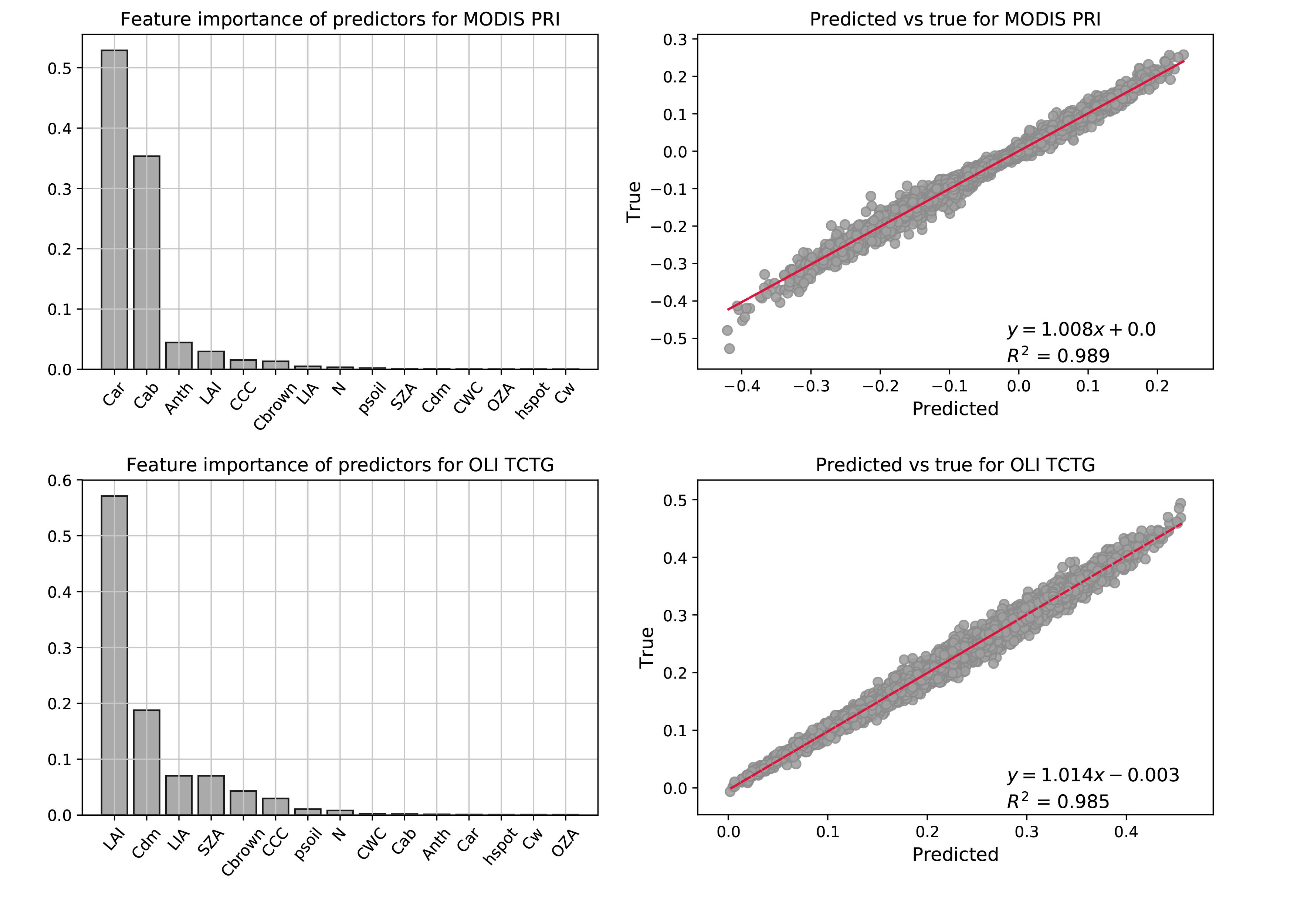
  • For most VIs, LAI is the most influential parameter, indicating that most VI variations are driven by LAI changes.
  • MODIS- and OLI-derived EVI is most sensitive to CCC, i.e., the product of Cab and LAI, but Sentinel-derived EVI is still most sensitive to LAI. This finding seems to support the previous conclusion that MODIS- and/or OLI–EVI are more appropriate for modeling GPP. In addition, it can be also concluded that the sensitivity of a VI depends on band settings of the used sensor.
  • EVI and NIRv are sensitive to Cdm, LIA, Cbrown, and SZA due to their sensitivity to NIR reflectance. Therefore, special attention should be paid when these two VIs are used across biomes with different canopy architecture and dry matter content.
  • Although both UNVI and TCTG are derived from all-band information, UNVI shows a stronger sensitivity to CWC. UNVI is therefore expected to perform better in agricultural drought monitoring models.
  • PRI and MTCI are most sensitive to Car and Cab, respectively.
Some uncertainties still exist for the GSA results in this study. A primary uncertainty is the limitation of the PROSAIL model. Because this is a case study based on the PROSAIL model, the results only apply for homogeneous canopies. For non-homogeneous canopies, such as forests, VIs can exhibit stronger anisotropy and show additional sensitivity to structural parameters, such as stem density, crown size, and fractional crown coverage [38]. Appropriate radiative transfer models for forest canopies exist, such as DART [39] and INFORM [40], but are not studied in our research, which focuses on homogeneous canopies. For example, a recent paper [6] shows large differences between the sensitivity of PROSAIL (for agricultural crops) and that of INFORM (for forests) to various canopy traits, demonstrating that our study needs to be extended to also cover those vegetation types. This seems even more important when considering the relatively large footprint of sensors such as OLCI and MODIS, as those sensors usually mix the signal stemming from several cover types. It should be also noted that for a model-based GSA, the results can be dependent on the design of the input parameters in the LUT. In this study, the range of Cab was set from 10 to 80 ug/cm2 on the basis of the fact that crop leaves have relatively high chlorophyll concentration. Therefore, the sensitivity of VIs to Cab is relatively weak compared to that in a recently published paper [6]. The boundaries of input parameters and the corresponding influences on GSA results should be further studied in future works. Sensor noise and the process of atmospheric correction were also neglected for the sake of convenience. A GSA based on canopy–atmosphere integrated RTM simulations may provide more realistic results [10]. With regard to the RF-based GSA method, although RF has been widely used to identify influential factors in situations without a physical model, its potential for GSA should be further studied, especially compared to variance-based methods. It should be noted that the RF-based method also supports a result-based GSA. Therefore, future studies can validate the GSA results with in situ data.
This study shows the sensitivities of several satellite-derived VIs that were used at relatively large scales based on PROSAIL simulation and RF-based GSA method. Combined variables, CWC and CCC, were introduced in the RTM-based GSA. The results may help to improve our understanding of the variability of these VIs across time and space. As an increasing number of studies is starting to use VIs at regional and global scales [8,16], the results presented here may help to understand the performances, sometimes unexpected, of VIs in different situations.

Author Contributions

S.W. designed the study and wrote the manuscript. D.Y., Z.L., L.L., C.H., and L.Z. provided useful suggestions during the preparation of the manuscript.

Funding

This research was funded by the National Key Research and Development program (2016YFB0500502), the Major Science and Technology Projects of XPCC (2018AA00402), the Innovation Team of XCPP’s Key Area (2018CB004) and the Key Research Program of Frontier Sciences, CAS (ZDBS-LY-DQC012).

Acknowledgments

The authors would like to thank anonymous reviewers and the academic editor for their constructive comments, which greatly improve the manuscript. The authors would like to thank Dr. J.Verrelst for the contribution of the ARTMO GUI tool.

Conflicts of Interest

The authors declare no conflict of interest.

References

  1. She, X.; Zhang, L.; Cen, Y.; Wu, T.; Huang, C.; Baig, M. Comparison of the Continuity of Vegetation Indices Derived from Landsat 8 OLI and Landsat 7 ETM+ Data among Different Vegetation Types. Remote Sens. 2015, 7, 13485–13506. [Google Scholar] [CrossRef] [Green Version]
  2. Huete, A.; Didan, K.; Miura, T.; Rodriguez, E.P.; Gao, X.; Ferreira, L.G. Overview of the radiometric and biophysical performance of the MODIS vegetation indices. Remote Sens. Environ. 2002, 83, 195–213. [Google Scholar] [CrossRef]
  3. Verrelst, J.; Rivera, J.P.; van der Tol, C.; Magnani, F.; Mohammed, G.; Moreno, J. Global sensitivity analysis of the SCOPE model: What drives simulated canopy-leaving sun-induced fluorescence? Remote Sens. Environ. 2015, 166, 8–21. [Google Scholar] [CrossRef]
  4. Ollinger, S.V. Sources of variability in canopy reflectance and the convergent properties of plants. New Phytol. 2011, 189, 375–394. [Google Scholar] [CrossRef]
  5. Xu, M.; Liu, R.; Chen, J.M.; Liu, Y.; Shang, R.; Ju, W.; Wu, C.; Huang, W. Retrieving leaf chlorophyll content using a matrix-based vegetation index combination approach. Remote Sens. Environ. 2019, 224, 60–73. [Google Scholar] [CrossRef]
  6. Morcillo-Pallarés, P.; Rivera-Caicedo, J.P.; Belda, S.; De Grave, C.; Burriel, H.; Moreno, J.; Verrelst, J. Quantifying the Robustness of Vegetation Indices through Global Sensitivity Analysis of Homogeneous and Forest Leaf-Canopy Radiative Transfer Models. Remote Sens. 2019, 11, 2418. [Google Scholar] [CrossRef]
  7. Zhang, L.; Jiao, W.; Zhang, H.; Huang, C.; Tong, Q. Studying drought phenomena in the Continental United States in 2011 and 2012 using various drought indices. Remote Sens. Environ. 2017, 190, 96–106. [Google Scholar] [CrossRef]
  8. Zhang, Y.; Xiao, X.; Wolf, S.; Wu, J.; Wu, X.; Gioli, B.; Wohlfahrt, G.; Cescatti, A.; van der Tol, C.; Zhou, S. Spatio-temporal Convergence of Maximum Daily Light-Use Efficiency Based on Radiation Absorption by Canopy Chlorophyll. Geophys. Res. Lett. 2018. [Google Scholar] [CrossRef]
  9. Gitelson, A.A.; Peng, Y.; Viña, A.; Arkebauer, T.; Schepers, J.S. Efficiency of chlorophyll in gross primary productivity: A proof of concept and application in crops. J. Plant Physiol. 2016, 201, 101–110. [Google Scholar] [CrossRef] [Green Version]
  10. Verrelst, J.; Vicent, J.; Rivera-Caicedo, J.P.; Lumbierres, M.; Morcillo-Pallarés, P.; Moreno, J. Global Sensitivity Analysis of Leaf-Canopy-Atmosphere RTMs: Implications for Biophysical Variables Retrieval from Top-of-Atmosphere Radiance Data. Remote Sens. 2019, 11, 1923. [Google Scholar] [CrossRef]
  11. Mousivand, A.; Menenti, M.; Gorte, B.; Verhoef, W. Global sensitivity analysis of the spectral radiance of a soil–vegetation system. Remote Sens. Environ. 2014, 145, 131–144. [Google Scholar] [CrossRef]
  12. Cannavó, F. Sensitivity analysis for volcanic source modeling quality assessment and model selection. Comput. Geosci. 2012, 44, 52–59. [Google Scholar] [CrossRef]
  13. Van der Tol, C.; Verhoef, W.; Timmermans, J.; Verhoef, A.; Su, Z. An integrated model of soil-canopy spectral radiances, photosynthesis, fluorescence, temperature and energy balance. Biogeosciences 2009, 6, 3109–3129. [Google Scholar] [CrossRef] [Green Version]
  14. Verrelst, J.; Malenovský, Z.; Van der Tol, C.; Camps-Valls, G.; Gastellu-Etchegorry, J.-P.; Lewis, P.; North, P.; Moreno, J. Quantifying Vegetation Biophysical Variables from Imaging Spectroscopy Data: A Review on Retrieval Methods. Surv. Geophys. 2018. [Google Scholar] [CrossRef]
  15. Zhang, L.; Qiao, N.; Baig, M.H.A.; Huang, C.; Lv, X.; Sun, X.; Zhang, Z. Monitoring vegetation dynamics using the universal normalized vegetation index (UNVI): An optimized vegetation index-VIUPD. Remote Sens. Lett. 2019, 10, 629–638. [Google Scholar] [CrossRef]
  16. Badgley, G.; Field, C.B.; Berry, J.A. Canopy near-infrared reflectance and terrestrial photosynthesis. Sci. Adv. 2017, 3, e1602244. [Google Scholar] [CrossRef]
  17. Baig, M.H.A.; Zhang, L.; Shuai, T.; Tong, Q. Derivation of a tasselled cap transformation based on Landsat 8 at-satellite reflectance. Remote Sens. Lett. 2014, 5, 423–431. [Google Scholar] [CrossRef]
  18. Tucker, C.J. Red and photographic infrared linear combinations for monitoring vegetation. Remote Sens. Environ. 1979, 8, 127–150. [Google Scholar] [CrossRef] [Green Version]
  19. Dash, J.; Curran, P.J. The MERIS terrestrial chlorophyll index. Int. J. Remote Sens. 2004, 25, 5403–5413. [Google Scholar] [CrossRef]
  20. Gamon, J.; Penuelas, J.; Field, C. A narrow-waveband spectral index that tracks diurnal changes in photosynthetic efficiency. Remote Sens. Environ. 1992, 41, 35–44. [Google Scholar] [CrossRef]
  21. Breiman, L. Random forests. Mach. Learn. 2001, 45, 5–32. [Google Scholar] [CrossRef]
  22. Liu, X.; Guanter, L.; Liu, L.; Damm, A.; Malenovský, Z.; Rascher, U.; Peng, D.; Du, S.; Gastellu-Etchegorry, J.-P. Downscaling of solar-induced chlorophyll fluorescence from canopy level to photosystem level using a random forest model. Remote Sens. Environ. 2018. [Google Scholar] [CrossRef]
  23. Peng, D.; Zhang, H.; Yu, L.; Wu, M.; Wang, F.; Huang, W.; Liu, L.; Sun, R.; Li, C.; Wang, D.; et al. Assessing spectral indices to estimate the fraction of photosynthetically active radiation absorbed by the vegetation canopy. Int. J. Remote Sens. 2018, 1–19. [Google Scholar] [CrossRef]
  24. Wu, C.; Niu, Z.; Gao, S. Gross primary production estimation from MODIS data with vegetation index and photosynthetically active radiation in maize. J. Geophys. Res. 2010, 115. [Google Scholar] [CrossRef] [Green Version]
  25. Peng, Y.; Gitelson, A.A. Remote estimation of gross primary productivity in soybean and maize based on total crop chlorophyll content. Remote Sens. Environ. 2012, 117, 440–448. [Google Scholar] [CrossRef]
  26. Gitelson, A.A.; Peng, Y.; Masek, J.G.; Rundquist, D.C.; Verma, S.; Suyker, A.; Baker, J.M.; Hatfield, J.L.; Meyers, T. Remote estimation of crop gross primary production with Landsat data. Remote Sens. Environ. 2012, 121, 404–414. [Google Scholar] [CrossRef] [Green Version]
  27. Zhang, Y.; Xiao, X.; Wu, X.; Zhou, S.; Zhang, G.; Qin, Y.; Dong, J. A global moderate resolution dataset of gross primary production of vegetation for 2000–2016. Sci. Data 2017, 4, 170165. [Google Scholar] [CrossRef]
  28. Xiao, X.; Hollinger, D.; Aber, J.; Goltz, M.; Davidson, E.A.; Zhang, Q.; Moore, B. Satellite-based modeling of gross primary production in an evergreen needleleaf forest. Remote Sens. Environ. 2004, 89, 519–534. [Google Scholar] [CrossRef]
  29. Berger, K.; Atzberger, C.; Danner, M.; Wocher, M.; Mauser, W.; Hank, T. Model-Based Optimization of Spectral Sampling for the Retrieval of Crop Variables with the PROSAIL Model. Remote Sens. 2018, 10, 2063. [Google Scholar] [CrossRef]
  30. Knyazikhin, Y.; Martonchik, J.; Diner, D.; Myneni, R.; Verstraete, M.; Pinty, B.; Gobron, N. Estimation of vegetation canopy leaf area index and fraction of absorbed photosynthetically active radiation from atmosphere-corrected MISR data. J. Geophys. Res. Atmos. 1998, 103, 32239–32256. [Google Scholar] [CrossRef] [Green Version]
  31. Knyazikhin, Y.; Schull, M.A.; Stenberg, P.; Mõttus, M.; Rautiainen, M.; Yang, Y.; Marshak, A.; Carmona, P.L.; Kaufmann, R.K.; Lewis, P. Hyperspectral remote sensing of foliar nitrogen content. Proc. Natl. Acad. Sci. USA 2013, 110, E185–E192. [Google Scholar] [CrossRef] [PubMed]
  32. Zhang, L.; Furumi, S.; Muramatsu, K.; Fujiwara, N.; Daigo, M.; Zhang, L. A new vegetation index based on the universal pattern decomposition method. Int. J. Remote Sens. 2007, 28, 107–124. [Google Scholar] [CrossRef]
  33. Zhang, L.; Liu, B.; Zhang, B.; Tong, Q. An evaluation of the effect of the spectral response function of satellite sensors on the precision of the universal pattern decomposition method. Int. J. Remote Sens. 2010, 31, 2083–2090. [Google Scholar] [CrossRef]
  34. Jiao, W.; Tian, C.; Chang, Q.; Novick, K.A.; Wang, L. A new multi-sensor integrated index for drought monitoring. Agric. For. Meteorol. 2019, 268, 74–85. [Google Scholar] [CrossRef] [Green Version]
  35. Jiao, W.; Zhang, L.; Chang, Q.; Fu, D.; Cen, Y.; Tong, Q. Evaluating an Enhanced Vegetation Condition Index (VCI) Based on VIUPD for Drought Monitoring in the Continental United States. Remote Sens. 2016, 8, 224. [Google Scholar] [CrossRef]
  36. Chou, S.; Chen, J.; Yu, H.; Chen, B.; Zhang, X.; Croft, H.; Khalid, S.; Li, M.; Shi, Q. Canopy-Level Photochemical Reflectance Index from Hyperspectral Remote Sensing and Leaf-Level Non-Photochemical Quenching as Early Indicators of Water Stress in Maize. Remote Sens. 2017, 9, 794. [Google Scholar] [CrossRef]
  37. Schickling, A.; Matveeva, M.; Damm, A.; Schween, J.; Wahner, A.; Graf, A.; Crewell, S.; Rascher, U. Combining Sun-Induced Chlorophyll Fluorescence and Photochemical Reflectance Index Improves Diurnal Modeling of Gross Primary Productivity. Remote Sens. 2016, 8, 574. [Google Scholar] [CrossRef]
  38. Widlowski, J.-L.; Mio, C.; Disney, M.; Adams, J.; Andredakis, I.; Atzberger, C.; Brennan, J.; Busetto, L.; Chelle, M.; Ceccherini, G. The fourth phase of the radiative transfer model intercomparison (RAMI) exercise: Actual canopy scenarios and conformity testing. Remote Sens. Environ. 2015, 169, 418–437. [Google Scholar] [CrossRef]
  39. Gastellu-Etchegorry, J.P.; Martin, E.; Gascon, F. DART: A 3D model for simulating satellite images and studying surface radiation budget. Int. J. Remote Sens. 2004, 25, 73–96. [Google Scholar] [CrossRef]
  40. Schlerf, M.; Atzberger, C. Inversion of a forest reflectance model to estimate structural canopy variables from hyperspectral remote sensing data. Remote Sens. Environ. 2006, 100, 281–294. [Google Scholar] [CrossRef]
Figure 1. Flow diagram showing the method of global sensitivity analysis of VIs used in this study. ARTMO: automated radiative transfer models operator.
Remotesensing 11 02547 g001
Figure 2. Feature importance scores of considered predictors given by random forest (RF) training. VIs are more sensitive to parameters with higher feature importance scores. It should be noted that UNVI and MTCI are shown in the same column because they are calculated, respectively, for two sensors.
Remotesensing 11 02547 g002
Figure 3. Feature importance scores and scatter plots between true and predicted values for MODIS-derived PRI and OLI-derived TCTG.
Remotesensing 11 02547 g003
Table 1. Designed look-up table of input variables of the PROSAIL radiative transfer model.
4SAILValues ([min, max])
Leaf are index (LAI) [m2/m2][0.1,8]
Hot spot parameter[0,0.5]
Leaf inclination angle (LIA) [degree][0,90]
Solar zenith angle (SZA) [degree)[20,70]
View zenith angle (VZA) [degree][−30,30]
Soil brightness parameter (psoil)[0.1]
PROSPECT-D
Anthocyanin content (Anth)[0,10]
Leaf structure parameter (N)[1,3]
Chlorophyll a+b content (Cab) [ug/cm2][10,80]
Carotenoid content (Car) [ug/cm2][0,20]
Dry matter content (Cdm) [g/cm2][0,0.02]
Water content (Cw) [cm][0,0.01]
Brown pigment content (Cbrown)[0,1]
Combined PredictorsCalculation
Canopy chlorophyll content (CCC)Cab × LAI
Canopy water content (CWC)Cw × LAI
Sampling method: Full Random Sampling
Table 2. Sensor–vegetation index (VI) combinations included in this study. Commonly used VIs considered in this study include the normalized difference VI (NDVI), enhanced VI (EVI), MERIS terrestrial chlorophyll index (MTCI), universal normalized VI (UNVI), near-infrared reflectance of vegetation (NIRv), photochemical reflectance index (PRI) and tasseled cap transformation greenness (TCTG). Formula and references of the considered VIs are also listed.
VIFormulaSensorReference
MODISOLIMSIOLCI
NDVI R NIR R R R NIR + R R [18]
EVI G R NIR R R R NIR + C 1 × R R C 2 × R B + L 1[2]
MTCI R NIR R RE R RE R R 2 [19]
UNVI C V a × C S C 4 C W + C V + C s 3 [15]
NIRv R NIR R R R NIR + R R × R NIR [16]
PRI R 531 R ref . R 531 + R ref . 4 [20]
TCTG R B 2 B 7 · C o e f . TCTG 5 [17]
1 Constant parameters for MODIS are used, with G = 2.5, C1 = 6, C2 = 7.5, and L = 1. 2 RRE stands for red-edge band reflectance, which corresponds to band5 (705 nm) and band11 (708.75 nm) of Multi-Spectral Instrument (MSI) and Ocean Land Color Instrument (OLCI), respectively. 3 Cv, Cs, Cw, and C4 stand for coefficients of vegetation, soil, water, and supplementary spectra. See [11] for detailed derivation. 4 MODIS band4 (555 nm) is used as a reference band. 5 RB2-B7 and Coef.TCTG stand for reflectance and TCTG coefficients vectors, respectively.

