Abstract
Color segmentation is one of the most thoroughly studied problems in agricultural applications of remote image capture systems, since it is the key step in several different tasks, such as crop harvesting, site specific spraying, and targeted disease control under natural light. This paper studies and compares five methods to segment plum fruit images under ambient conditions at 12 different light intensities, and an ensemble method combining them. In these methods, several color features in different color spaces are first extracted for each pixel, and then the most effective features are selected using a hybrid approach of artificial neural networks and the cultural algorithm (ANN-CA). The features selected among the 38 defined channels were the b* channel of L*a*b*, and the color purity index, C*, from L*C*h. Next, fruit/background segmentation is performed using five classifiers: artificial neural network-imperialist competitive algorithm (ANN-ICA); hybrid artificial neural network-harmony search (ANN-HS); support vector machines (SVM); k nearest neighbors (kNN); and linear discriminant analysis (LDA). In the ensemble method, the final class for each pixel is determined using the majority voting method. The experiments showed that the correct classification rate for the majority voting method excluding LDA was 98.59%, outperforming the results of the constituent methods.
1. Introduction
It is a well-known fact that agricultural engineering is one of the main areas of application for remote sensing technologies [1]. These can include spaceborne, airborne and terrestrial platforms, with applications in crop monitoring, water management, fertigation, harvesting, and decision making in general. In particular, using automated or semi-automated harvesting methods is not only economically cost effective, but also more efficient than traditional methods, and significantly reduces the harvest time, as observed in some of the early works on automated harvesting [2]. There are currently several methods of automated harvesting using different remote image capture techniques. The most common are based on the use of harvesting robots using image-processing modules [3,4,5,6,7]. Since farming robots need to work in uncontrolled environments, both natural lighting conditions and complex background have to be considered, making segmentation particularly sensitive and complicated. Direct sunlight causes images and frames to be extremely intense in the sunny areas and poorly lit in the shaded areas. This could make the segmentation system to be confused [8]. Moreover, other factors, such as complex background, partial occlusion, and poor capture quality [9], must also be considered.
Regarding these applications, Miao et al. [10] captured 380 RGB images in three morning, noon and evening lighting conditions for farmland recognition and classification, with a resolution of 2576 × 1932 pixels. Then, from each image, eight features were extracted that include the three components of the HSL color space, the second and third components of HSV, and the three components of HSI. The dimensionality of the data was reduced using 5 eigenvectors extracted with principal components analysis. Finally, images were classified using a radial basis function neural network. The results showed that this classification system was able to classify images in sunny and cloudy days with an accuracy of 84.58% and 68.11%, respectively. However, this classification accuracy is not enough for a practical use in machine vision systems, as it would result in many errors.
Zhao et al. [11] proposed a method for detecting immature green citrus fruits in orchards. This method was a combination of color features and the sum of the absolute conversion differences. To develop the detection algorithm on natural conditions, 126 images were taken in Florida, USA, at several different times of the day. The resulting images had a very high resolution of 3636 × 2736 pixels. From these images, 58 were used for training and the other 68 for a support vector machine (SVM) classification test. A comparative chromatic red and blue map was created and combined with the hue image extracted after the histogram alignment. Next, to identify potential fruit pixels, the sum of the absolute conversion difference and a block matching method were used. Finally, the results showed that the proposed algorithm had a detection accuracy of 83%.
Another interesting method for litchi fruit segmentation in stereo images under different lighting conditions has been proposed by Wang et al. [12]. This method involved the use of advanced wavelet transform to normalize object surface lighting. The Retinex-based image enhancement algorithm [13] was then used to highlight the fruit object from the normal brightness image. Finally, the fruit image was analyzed using k-means clustering. The results obtained indicated that this algorithm can be efficient in dealing with different light effects. Also, Sabzi et al. [14] proposed an apple segmentation algorithm under direct sunlight in garden conditions. To find the appropriate color space to perform part of the segmentation, 17 color spaces containing 51 color channels were examined. The main goal was to find the color space with the least number of colors to apply the threshold. One of the most important parts of this research was the arrangement of different segmentation steps. By applying color segmentation, texture analysis, and intensity conversion, a large number of background pixels were removed and apples were segmented in the images. The accuracy achieved by the segmentation algorithm was 98.92%.
Since shadows are problematic for segmentation, Weiyue et al. [15] presented a new algorithm for identifying and removing shadows in a system for apple segmentation. They combined group pixels and edge maps to produce hyper-pixel blocks with precise boundaries. A correlation matrix was used to obtain the ultra-metric counter map for shadow detection; a relative method for shadow removal was then used. Results showed that the mean square error decreased from 7.9% to 6.4% when using the edge probability map. Using this shadow removal algorithm, the segmentation accuracy was improved by 10%. The average processing time was 0.59 s, so the proposed algorithm was efficient to detect apples in orchards under natural light conditions. Finally, it is also worth mentioning the work by Sengupta and Lee [16], who developed an algorithm for identifying green tangerines under natural conditions. The shape and texture features were two integral parts of the algorithm. The shape attribute was used to identify as many fruits as possible. Tissue classification was also used to remove false positives. The reported fruit recognition rate was 80.4%.
More recently, Wang et al. [6] proposed an improvement in the methods of fruit localization for harvesting robots using binocular stereo images. The proposed method uses the Faster region-based convolutional neural network (R-CNN), which is able to achieve a recognition rate of 96.33% in six different conditions. Then, the window zooming method was applied to match detections in the stereo par, obtaining a 93.44% of correct matches, allowing the computation of the 3D position of the fruits. This is a breakthrough compared to other previous works of the authors, such as [17] for the detection of grape clusters in vineyards, [18] for green grape, and [19,20] for the case of litchi fruits. An interesting description of other current research works in fruit detection and localization can be found in [6].
As can be seen, segmentation is a very important step in many machine vision systems of remote imaging in agriculture. This step must be performed with high precision because the subsequent steps of the system depend on the accuracy of segmentation. For this reason, the purpose of the present study is to compare different pixel-by-pixel segmentation methods and their combination in an ensemble with a majority voting rule. The ensemble consists of different heterogeneous classifiers: hybrid artificial neural network-imperialist competitive algorithm (ANN-ICA); hybrid artificial neural network-harmony search (ANN-HS); support vector machines (SVM); and k nearest neighbors (kNN); and linear discriminant analysis (LDA), which can also be considered a baseline method. By using different classification techniques, the individual effectivity of these methods can be analyzed and compared. The system is applied to the segmentation of plum fruits in orchards in different ripeness stages under natural conditions.
2. Materials and Methods
The system proposed in this paper is based on color analysis, pixel-by-pixel segmentation, and an ensemble of classifiers. Figure 1 presents a diagram of main stages of the system. The key aspects are the definition of the color features to be extracted, the selection of the most effective features, the individual classification with the five basic classifiers, and the combination using a voting method. All of these operations are applied at a pixel-level. Previously, a training/test set of pixels has been obtained by a human expert, dividing them into two groups: plum fruit pixels, and background pixels. Therefore, we have a binary classification problem.
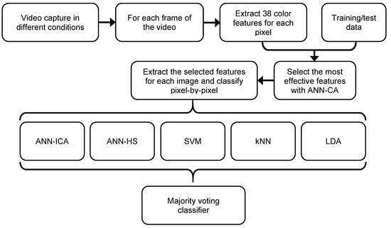
Figure 1.
Diagram of the steps of the original approach for plum fruits segmentation.
2.1. Video Recording and Data Collection
The first step of the research process is to capture the videos in different environmental conditions. For this purpose, during the years 2018 and 2019, a total of 12 videos were recorded under different natural light intensities at different stages of plum fruit growth. The videos were produced from different fruit gardens in Kermanshah province, Iran (34°18′48.87″N, 47°4′6.92″E) using a color GigE industrial camera model DFK 23GM021 (Imaging Source Europe GmbH, Bremen, Germany), with a 1/3 inch Aptina CMOS MT9M021 sensor (ON Semiconductor, Aurora, CO, USA) and a spatial resolution of 1280 × 960 pixels. The mounted lens was model H0514-MP2 (Computar CBC Group, Tokyo, Japan), with f = 5 mm and F1.4. They were captured manually, simulating the route of a terrestrial harvesting robot.
Figure 2 shows eight image samples displaying different fruit growth conditions, as well as different light intensities. On the other hand, Table 1 shows the main characteristics of these videos. Finally, 49,347 pixels were manually extracted and classified from different frames by a human operator, classifying them in plum or background class. Of these, 34,543 pixels (70% of the data) were used to train the proposed algorithm, and the remaining 14,804 pixels (30% of the data) to test and validate the system.
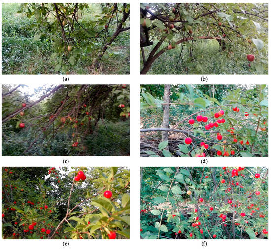
Figure 2.
Different frames extracted from the recorded videos from different orchards. These frames correspond to the videos described in Table 1 with light intensities: (a) 826 lux; (b) 593 lux; (c) 342 lux; (d) 467 lux; (e) 1563 lux; (f) 1963 lux; (g) 639 lux; (h) 287 lux.

Table 1.
Characteristics of the videos taken from the plum orchards under different conditions.
Since the purpose of the current research is to compare different segmentation algorithms under natural conditions, the appearance and complexity of the background is very important. Some of these backgrounds include leaves, branches, leaf tail, clear sky, cloudy sky, green vegetation, yellow plants, dense leaves and soil. Due to the variations in background objects, it is difficult to develop a comprehensive segmentation algorithm; but if the development of such an algorithm is achieved, many operations related to machine vision systems operating in different environmental conditions can be performed with high precision.
2.2. Selection of the Most Effective Color Features
The proposed method is based on color, as a powerful and effective feature widely applied to computer vision in agriculture [21]. Different color spaces, including RGB, HSV, HSL, HSI, L*a*b*, L*u*v*, XYZ, YCbCr, YUV, YIQ, CMY and L*C*h, were used to extract the different color properties of the pixels. The first, second and third components were extracted for all these color spaces; so, since there are 12 color spaces, 36 color features were extracted from each pixel.
C* channel is also defined as the color purity index, and it was introduced by Clerici et al. in [22]. Observe that texture features were not included in the system, since the plums typically appear with a small size and there is no characteristic texture on them.
Since the purpose of the segmentation algorithm is to be used by a robot in real-time, the computational efficiency is a key parameter. It is not feasible to use all the predefined features, even if it does not interfere with the algorithm’s performance, since computing these 38 properties for each pixel would be time consuming. To solve this problem, the most effective color features must be chosen. In this regard, a hybrid method of artificial neural networks (ANNs) and the cultural algorithm (CA) was used to select the most effective color properties. Table 2 shows the parameters used in the multilayer perceptron ANN to select these properties.
Table 2.
Definition of the color models used in the present research. The equations to obtain these channels from the original RGB values are shown.
The CA metaheuristic, like the genetic algorithms (GA) [23,24,25,26], performs the control of an optimization process. GA considers natural and biological evolution, while CA considers cultural evolution and the impact of cultural and social conditions that ultimately lead to a model for solving a problem. In a society, everyone who is most considered will directly and indirectly have the most impact on cultural evolution. In fact, these people will influence the way society speaks, walks, dresses, and so on. Thus, the ultimate goal of this algorithm is to find and develop these elites for cultural evolution [27].
The procedure of the hybrid approach ANN-CA is as follows. All the color features extracted for each pixel are considered. The process selects small vectors of properties, for example, vectors with two, three, or four features, with the corresponding output class, fruit or background. For each selection of properties, the vectors are sent to a multilayer perceptron ANN with the hidden layer properties shown in Table 3. The method divides the inputs in 70% for training, 15% for validation, and 15% for testing. The mean squared error (MSE) of each input vector is recorded, obtaining the average MSE of each selection of features. Finally, the vector with the least MSE is selected as the optimal vector, and the corresponding properties are selected as the most effective color features. The task of the CA metaheuristic is to generate the different combinations of features in a controlled way.
Table 3.
Parameters used in the multilayer perceptron artificial neural network (ANN) to select the most effective features.
2.3. Underlying Color Classifiers
As depicted in Figure 1, the proposed segmentation method is based on an ensemble of different classifiers, which are then combined with a majority voting step. That is, each pixel is first classified with the five underlying methods, and the final class is obtained with the majority rule. For example, if three of the classifiers consider a pixel as fruit and the other two consider it as background, the final class of the pixel is fruit. This procedure has the additional advantage that it allows us to compare the accuracy obtained by each basic classifier. These are explained in the following subsections.
2.3.1. Hybrid Artificial Neural Network-Imperialist Competitive Algorithm (ANN-ICA)
The imperialist competitive algorithm (ICA) is a metaheuristic algorithm based on cultural, social and political evolution. In this algorithm, all countries are looking for a general optimal point to solve the optimization problem [28]. In our case, the task of ICA is to determine the optimal values of the multilayer perceptron ANN parameters. This network has 5 customizable hyperparameters that define the structure of the network and influence its performance: the number of hidden layers; the number of neurons per layer; the transfer function of each layer; the back-propagation network training function; and the weight/bias-back-propagation learning function.
The range of neurons selected was between 0 and 25 for each hidden layer, meaning a 0 that there is no hidden layer. The number of hidden layers is between 1 and 3. For each layer, a transfer function is required. In this study, this transfer function will be selected from the 13 transfer functions available in MATLAB neural network toolbox (MathWorks) [29], such as tangent sigmoid, log-sigmoid or linear. The next hyperparameter for the ICA is the function of the back-propagation network training; this will be selected from the 19 functions available also in the cited toolbox. Finally, the weight/bias backpropagation learning function was selected from 15 different available functions.
The procedure is that, initially, the ICA algorithm considers a vector with the same number of parameters as a vector with a minimum of 4 and a maximum of 8 members. Each member represents a parameter. For example, a vector of the form x = {19, radbas, trainscg, learnsomb} indicates that the ANN under study has one hidden layer with 19 neurons, with radial basis transfer function, scaled conjugate gradient backpropagation training function, and self-organizing map weight learning function. The obtained average MSE determines the performance of the ANN for each of the vectors transmitted, so that the vector with the least average MSE is selected as the optimal vector to adjust the ANN parameters. As in the other methods, the input samples are divided in 70% for training, 15% for validation, and 15% for testing.
2.3.2. Hybrid Artificial Neural Network-Harmony Search (ANN-HS)
This method is also a hybrid approach where a meta-heuristic algorithm is used to find the optimal hyperparameters of an ANN. In this case, the harmony search (HS) procedure imitates the natural process of music optimization. In the making of a song, the beauty of the song determines the step of each musical device; in other words, each device must be optimized. Therefore, the value of the objective function is determined by the values of the problem variables [30]. The process to optimize the ANN hyperparameters is very similar to the process described in the previous subsection, with the only difference in the order in which the vectors are selected by the algorithm. The maximum number of hidden layers, neurons per layer, and the available functions are the same as in ANN-ICA.
2.3.3. Support Vector Machines (SVM) Classifier
Support vector machines [31] are one of the most popular supervised learning methods used for regression and classification problems. This method performs classification operations using linear classification of data. This way, it attempts to find the hyperplane of maximum separability of the samples of the two classes. Using a kernel function, the input data is implicitly mapped into a high-dimensional space, thus allowing not linear decision boundaries.
In the experiments, the kernel function for the SVM classifier was a simple dot product. The soft margin parameter, or C value, was selected to 1. These values were empirically obtained through a series of experiments with the same dataset, where the kernel functions tested were: dot product, polynomial, radial basis function (RBF) and sigmoid. The values tested for C were: 0.01, 0.1, 1 and 10.
2.3.4. k-Nearest Neighbors (kNN) Classifier
k-nearest neighbors is another non-parametric method used for classification [32,33]. Similar to SVM, it is also a sample-based method. This algorithm classifies each new sample based on the closest properties of other samples in its neighborhood. In short, this method works as follows, given a parameter k indicating the number of neighbors to be considered:
1. Calculate the distance between the input sample and all the training samples. This distance is usually measured in terms of the Euclidean distance. If X1 = (X11, X12 … X1n) and X2 = (X21, X22 … X2n) are two given tuples, then the Euclidean distance between them is calculated as:
2. Sort the training samples in ascending order of the distance, selecting the k nearest samples.
3. The class with the greatest number of neighbors in the previous set of k samples is assigned to the input sample.
Although, in theory, this method requires the distance to all the training samples to be computed, the process can be optimized to reduce the computational time required, such as using the condensed nearest neighbor rule [34]. In our case, considering the low dimensionality of the input vectors and the large number of training samples, the value of k was selected to 5 in the experiments. This value was empirically obtained in a trial and error process, testing different odd values from 1 to 11.
2.3.5. Linear Discriminant Analysis (LDA) Classifier
The last method used in the ensemble classifier is LDA, which is another well-known technique. LDA tries to find a hyperplane to separate the samples of both classes, considering the mean and variance of them. The method of LDA can be performed in three ways: direct, hierarchical and stepwise. The step-by-step approach is more widely used by researchers because it incorporates independent variables based on predictive power. Therefore, the stepwise method was used in this study [35].
In our research, LDA is used as a baseline method for the comparison of the other more advanced techniques. For this reason, the color features used in the LDA space are the same as in the other classifiers, instead of selecting different features for each classifier. It has been observed in some of our previous research that many non-linear decision boundaries appear in low dimensional color spaces, especially when a complex and varied background is considered [21]. Thus, LDA is not expected to achieve great results, but it is interesting to compare its accuracy.
2.4. Combination of the Ensemble Classifier
In an ensemble of classifiers, each input sample is processed by the constituent classifiers, and then their results are combined according to a predefined rule. In our case, the outputs of the basic classifiers are combined using a majority voting method. This means that a pixel is assigned to a certain class when a half or more classifiers produced that class. Other combination techniques have been proposed in the literature, such as the variation of weighted voting [36], although they were not considered adequate for the present application.
2.5. Performance Evaluation Parameters of the Classifiers
2.5.1. Performance Parameters Based on the Confusion Matrix
The confusion matrix is a table that relates the real and predicted instances achieved by a classifier. It is a square matrix with a row and column for each existing class; in our case, it is 2 × 2. The matrix itself is useful for analyzing the performance of the classifier. In addition, using this matrix, different metrics can be defined and applied, as discussed below:
Sensitivity or Recall. Percent of the correct samples that have been correctly identified:
Accuracy or correct classification rate or overall accuracy. Total percentage of the correct system responses:
Specificity. Percentage of negative samples that are correctly identified:
Precision. Percentage of correctly identified outputs that are actually true:
F_measure. Harmonic mean of the recall and the precision:
Here, the positive class is the fruit (the object of interest) and the negative class is the background. Therefore, TP is equal to the number of samples of plum fruit that are correctly classified; TN is the number of samples of the background class that are correctly classified; FN is the number of fruit pixels misclassified as background; and FP is the number of background pixels misclassified as fruit. It has to be noted that some measures should not be analyzed by themselves. For example, a naïve system that always says true would have a recall of 100%, while a system that always says false would have a specificity of 100%.
2.5.2. Receiver Operating Characteristic
Receiver operating characteristic (ROC) charts are used to evaluate the performance of classification systems. These charts are plotted in a coordinate system with two axes, the horizontal axis being the FP rate, and the vertical axis being the TP rate achieved by the classifier. The number of graphs is the number of classes available, although in the case of two classes both curves are equivalent. An ideal ROC curve would be a single point with FP = 0 and TP = 1, indicating perfect classification accuracy. Therefore, a diagram looking like orthogonal indicates a higher performance [37]. The points of the ROC represent the different configurations of the classifier, from the most restrictive (near the point with TP = 0, FP = 0) to the most permissive (point TP = 1, FP = 1). If the classification method cannot be configured, it would only have a working point, so the ROC would consist of two straight segments. This happens, for example, with SVM and kNN classifiers.
A useful criterion that summarizes the performance of segmentation based on the ROC chart is the area under the curve (AUC), which is the integral of the ROC curve. The minimum value for this criterion is 0.5 (a random classifier) and the maximum is 1 (a perfect classifier).
3. Results and Discussion
This section describes the experimental results obtained, and discusses the main findings from these experiments. First the partial results of the intermediate steps are presented, that is, the selection of the most effective color features and the configuration of the ANNs with ICA and HS metaheuristic algorithms. Then, the accuracy of the basic classifiers and the ensemble method are analyzed using the evaluation parameters previously described. Finally, the results obtained are compared with other state-of-the-art methods available in the literature.
3.1. Selection of the Color Features and Configuration of ANN-ICA and ANN-HS
As described in Section 2.2, the first step of the process is to select the most effective color features for the problem of interest, among the 38 available color channels. This is done with a hybrid approach ANN-CA, which tests different combinations of channels. Finally, the most effective features automatically selected were channel b* in the L*a*b* color space, and the color purity index, C*, from the L*C*h space, which is also derived from a* and b* channels (see Table 1). This predominance of the L*a*b* color space has also been reported in other applications of computer vision in agriculture [38]. However, it should be noted that these results may depend on the specific application domain.
Another interesting result to discuss is that the process ends with the selection of only 2 color features. Observe that this number is not fixed a priori. The ANN-CA process tests different combinations between one and six channels. However, only two channels are selected as the optimal configuration. This could indicate that a greater number of channels is prone to produce overfitting, thus leading to poor classification results. This conclusion is consistent with [38], where all the combinations of one, two, and three channels in nine standard color spaces for a problem of plant/soil segmentation are tested; the reported results indicate that the optimal selection consists of the channels L* and a* in L*a*b*. Therefore, a reduced number of features is enough for an effective use of color in segmentation problems. This limitation is also very useful to achieve good computational efficiency in the algorithms.
The other applications of hybrid approaches are in the configuration of the hyperparameters of the ANNs for classification, with ANN-ICA and ANN-HS, using the two features mentioned. The optimal configurations for ANN-ICA and ANN-HS are shown in Table 4 and Table 5, respectively.
Table 4.
Optimal values of ANN parameters determined by imperialist competitive algorithm (ICA).
Table 5.
Optimal values of ANN parameters determined by harmony search (HS) algorithm.
In both cases, the optimal configuration of the ANNs consists of only two hidden layers with a similar number of neurons, although the process tests bigger sizes. This result may be related to the fact that the input tuples consist of only two values, so the necessary decision boundaries can be created with only 2 layers between 10 and 24 neurons per layer.
3.2. Classification Results of the Ensemble Method and the Basic Classifiers
In order to evaluate the reliability of the classifiers, 275 repetitions were performed for each method, that is, 275 independent executions of the training/testing process. The proposed ensemble method originally consisted of the 5 classifiers presented: ANN-ICA; ANN-HS; SVM; kNN; and LDA. However, it was observed that the poor results of LDA (as presented below) seriously affected the global performance of the ensemble. Therefore, we decided to include a new majority voting method removing LDA from the ensemble.
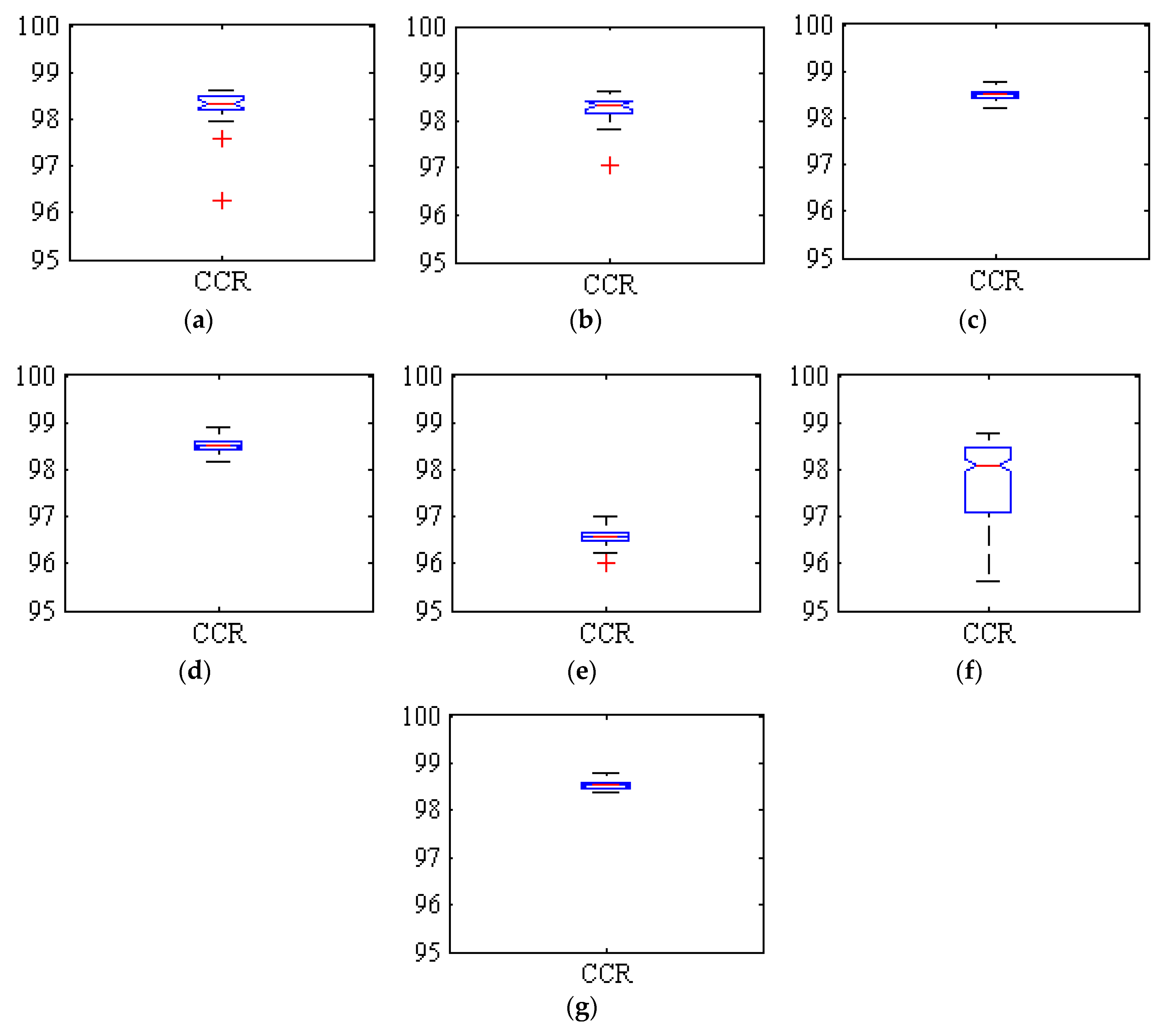
Figure 3 shows boxplots of the correct classification rates (CCR), or overall accuracy, achieved by all the classifiers in the fruit/background segmentation for the 275 executions. The red crosses indicate exceptionally low or high execution results.
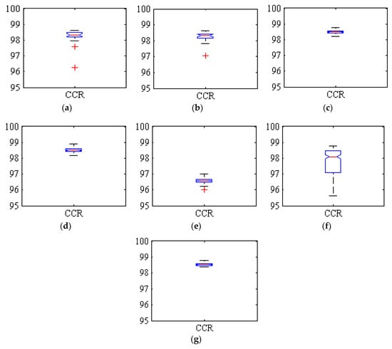
Figure 3.
Boxplots of the correct classification rate (CCR) obtained by the classifiers for the 275 executions. (a) Hybrid ANN-ICA; (b) Hybrid ANN-HS; (c) SVM; (d) kNN; (e) LDA; (f) Voting method with LDA; (g) Voting method without LDA.
In all cases, the accuracy achieved was always above 96%, with best average results above 98%. Some methods were more consistent in these good results (i.e., the variance between executions is very small), such as SVM, kNN and specially the ensemble method, while the results of LDA were also consistent but significantly lower, below 97%. This compactness of the boxplots indicates the close proximity of the values in different executions, and consequently the high reliability of the classification. The two hybrid methods based on ANN (i.e., ANN-ICA and ANN-HS) also produced good results, but with a bigger variance between executions. On the other hand, the original ensemble classifier including LDA was clearly affected by the errors of the poorest methods; it had an average accuracy of only 97.68%, and the variance was larger than that of all the basic classifiers. However, removing LDA from the ensemble, the method is able to improve the results of the constituent classifiers, both achieving a good average accuracy of 98.59%, and a very low variance.
Table 6 presents the confusion matrices and the error rates per class for the test data in the 275 repetitions for all the classifiers. Since there are 14,804 test samples and 275 iterations performed, the total accumulated is equivalent to 4,071,100 samples (32.6% of the fruit class, and 67.4% background).
Table 6.
Confusion matrices, rates of error by class, and CCR for all the classifiers and the 275 repetitions.
These matrices allow a deeper insight into the results. Since the number of background samples is bigger than fruit samples, all the methods tend to over-classify the new inputs into the background class, producing higher error rates for this class, i.e., the number of FP and FN samples are not balanced. This is especially prominent in the LDA method, where the error in the fruit class is 31 times bigger. Only the SVM classifier exhibits a balanced accuracy, with 1.99% error in the fruit class and 1.28% in the background. The CCR of SVM (98.49%) is lower than that kNN (98.50%), but the difference is not significant. The imbalance in the results of the ensemble without LDA is relatively small (as compared, for example, with the two ANN methods), and it also outperforms the CCR of the constituent methods.
The imbalance observed in the accuracies for the different classes is most probably due to the imbalance in the dataset between the fruit and background samples. In our case of study, the plums only represent about 2% of the whole images. Thus, the plum class has been oversampled, with 33% and 67% samples of the fruit and background classes, respectively. But although the imbalance of the samples has been reduced, there are still twice as many samples of the background class. It would be interesting to perform an additional subsampling of the background class, using for example half of the samples. However, while this could reduce the classification bias, the overall classification accuracy of the images would be smaller, since they contain about 98% of background.
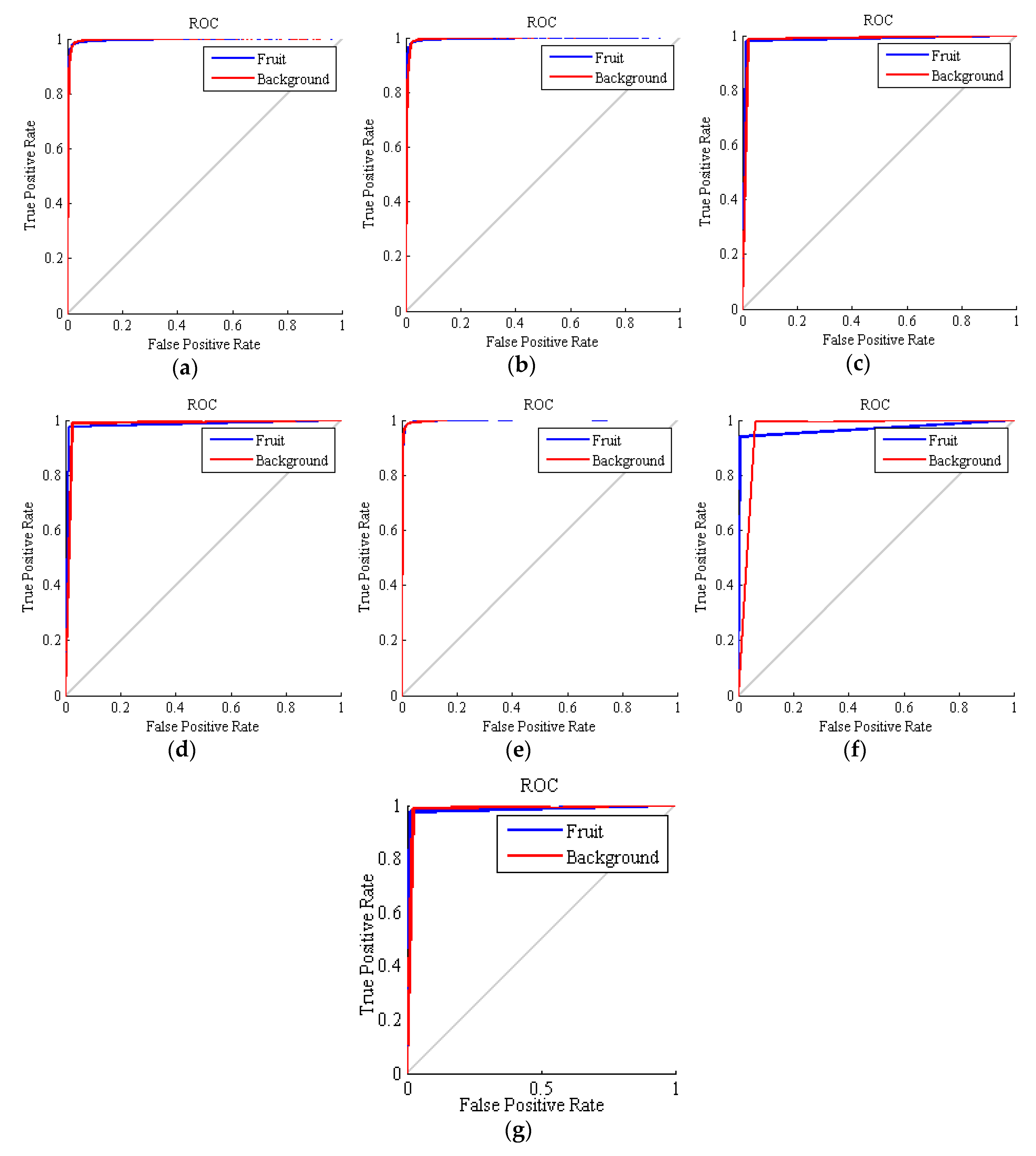
The ROC curves obtained for all the methods are depicted in Figure 4. In these curves, the closer the curve is to the vertical, the higher the performance. In general, all the ROCs exhibit good results, but the accuracy of SVM is again the best of all the basic methods. As mentioned above, the curves of SVM, kNN and the ensemble classifiers are piecewise linear, since these techniques cannot be adjusted to be more or less restrictive. This fact makes that, even that these methods achieve a good accuracy, the AUC parameter is degenerated since it loses its original meaning of measuring different configurations of the classifier.
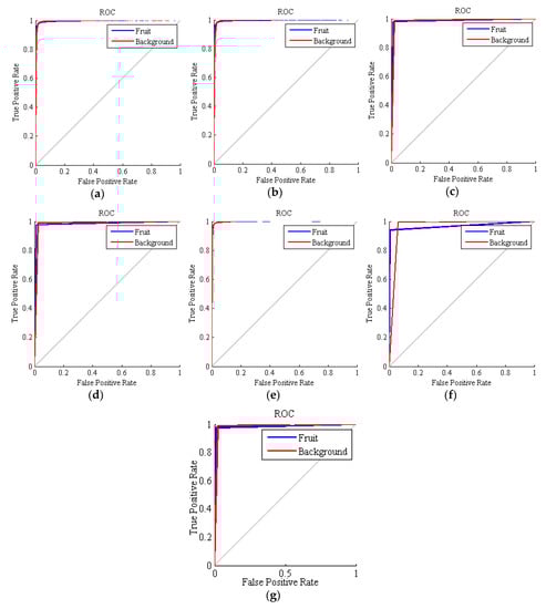
Figure 4.
Receiver operating characteristic (ROC) curves obtained by the classifiers for the 275 executions. (a) hybrid ANN-ICA; (b) hybrid ANN-HS; (c) support vector machines (SVM); (d) k nearest neighbors (kNN); (e) linear discriminant analysis (LDA); (f) voting method with LDA; (g) voting method without LDA.
Finally, Table 7 contains the six performance evaluation criteria obtained in the experiments. As can be seen, except for the LDA classifier and the original voting method, all the values were above 96%, indicating high performance in the fruit/background classification in general. The high recall value of LDA is due to the fact that it tends to overclassify in the background class; so this cannot be considered a good result, when considering its low specificity. Since LDA performs a simple linear separation of the samples, its poor results indicate that the samples cannot be classified with a linear decision boundary. This fact seriously affects the results of the voting method with LDA. The two ANN methods also present a certain tendency to overclassify in the background class, which was evident from their low precision. However, the majority voting method without LDA is able to reduce this bias; it achieves high results for recall and precision, which are transformed in an F_measure of 98.95%.
Table 7.
Performance evaluation criteria of the classifiers and the 275 executions.
As a concluding remark, it is evident that the ensemble method without LDA is able to improve significantly the accuracy of the constituent methods. It exhibits a better overall accuracy and greatly reduces the over-classification tendency of the ANN methods. The standard deviation of the accuracy also indicates a great consistency in these good results, as previously mentioned. The LDA is the worst of all the methods, and the accuracy obtained was only 96.57%. This fact justifies that LDA should be removed from the ensemble, since it only worsens the final result, producing also a standard deviation nearly ±2.
Another interesting aspect to consider is that the application of the proposed ensemble method without LDA requires the execution of all four classifiers that compose it. It is still unclear whether the computational cost of the ensemble and the majority voting rule is or is not beneficial, taking into account the small increment in the accuracy of only 0.1%. Alternatively, the SVM classifier also achieves good results, with low standard deviation, and is computationally more efficient. This is another advantage with respect to the kNN, which requires storing and processing all the training samples in the classification, while the SVM only stores the selected support vectors. In any case, the bottleneck of the process is most probably the color space conversion; since all the methods rely on L*a*b*, the application of the ensemble method could be justified. More experiments concerning the computational efficiency, which are outside the scope of this paper, would be needed.
3.3. Final Proposed Method and Comparison with the State-of-the-Art
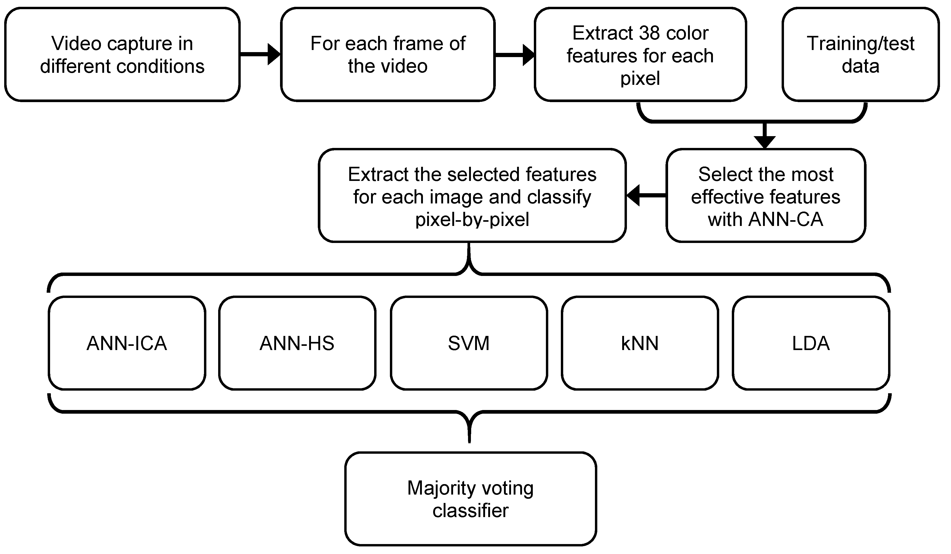
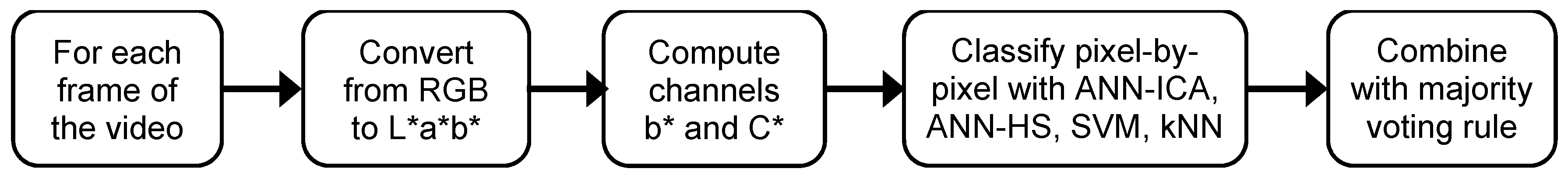
After examining the experimental results, the final algorithm for the segmentation of plum fruits from the background in the videos of plum orchards is illustrated in Figure 5. As previously explained, this method is based on the ensemble of the four classifiers excluding LDA, which is the most accurate and reliable method, and with a good balance in the accuracy per class. This scheme assumes that the basic classifiers have been trained, so it only contains the steps for the classification of a new frame.
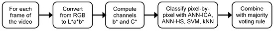
Figure 5.
Diagram of the proposed algorithm for plum fruits segmentation. A sample video of the results can be accessed in: https://youtu.be/PoSrkz5PSJI.
Table 8 contains a comparison of the correct detection rate of the proposed method with other methods presented by different researchers in the literature. According to this table, the proposed method is more accurate than those proposed by the other works. However, this conclusion should be taken with caution. A direct comparison of the results is not possible, because the application domain is different, the input images are also different, and in some cases the problem is not exactly the same.
Table 8.
Comparison of the accuracy of the segmentation algorithms reported in different works.
4. Conclusions
This study has addressed the segmentation of plum fruits in videos recorded under natural lighting conditions, for application in remote sensing problems. The method works at a pixel level, using color features. Five basic classifiers have been analyzed, and the combination of four of them using a majority voting rule. Two methods are hybrids of ANN and metaheuristics (ANN-ICA and ANN-HS), two methods are non-parametric sample-based methods (SVM and kNN), and the last method is based on linear discriminant analysis (LDA), which was not included in the ensemble due to its poor results.
Pixel-by-pixel analysis is highly efficient, because it measures the color properties of each pixel. The selection of the most effective color features has shown that a reduced number of parameters can be useful to obtain an accurate result. In our case, channel b* of L*a*b* and the color purity, C*, from L*C*h were found to be the optimal color properties.
The single methods were able to achieve very accurate results. SVM and kNN are the optimal selections, being able to produce 98.49% and 98.50% correct classification. The methods based on ANN also obtained good results, above 98.2%, but suffered from a certain imbalance in the accuracies per class. All of these methods were outperformed by the ensemble method without LDA, which removes this imbalance and achieves an overall accuracy of 98.59%.
An interesting aspect to consider in future research is the trade-off between accuracy and computational efficiency. While the proposed ensemble technique is able to improve the results of the constituent methods, it also accumulates the cost of all of them. The particular characteristics of the hardware, the minimum image resolution, and the required speed should be taken into account. Another promising future line of work is the comparison with other ensemble techniques, such as random forests, that has been successfully applied to similar problems, and the inclusion of other basic methods, such as logistic regression and feature weighting. Post-processing techniques could also be applied to improve the results of the pixel-by-pixel segmentation.
Author Contributions
Conceptualization, R.P. and S.S.; Methodology, R.P., S.S., M.H.-H., J.L.H.-H. and G.G.-M.; Software, S.S.; Validation, R.P., S.S., M.H.-H., D.K. and J.M.M.-M.; Formal Analysis, R.P., S.S. and G.G.-M.; Investigation, R.P., S.S., M.H.-H., J.L.H.-H., D.K., G.G.-M. and J.M.M.-M.; Resources, R.P. and S.S.; Writing—Original Draft Preparation, R.P. and S.S.; Writing—Review & Editing, M.H.-H., J.L.H.-H., D.K., G.G.-M. and J.M.M.-M.; Supervision, R.P.; Project Administration, R.P., G.G.-M. and J.M.M.-M.; Funding Acquisition, M.H.-H., J.L.H.-H., G.G.-M., D.K. and J.M.M.-M.
Funding
This research was funded by the Spanish MICINN, as well as European Commission FEDER funds, under grant RTI2018-098156-B-C53. This project has also been supported by the European Union (EU) under Erasmus+ project entitled “Fostering Internationalization in Agricultural Engineering in Iran and Russia” [FARmER] with grant number 585596-EPP-1-2017-1-DE-EPPKA2-CBHE-JP.
Conflicts of Interest
The authors declare no conflict of interest. The funders had no role in the design of the study; in the collection, analyses, or interpretation of data; in the writing of the manuscript, or in the decision to publish the results.
References
- Atzberger, C. Advances in remote sensing of agriculture: Context description, existing operational monitoring systems and major information needs. Remote Sens. 2013, 5, 949–981. [Google Scholar] [CrossRef]
- Jiménez, A.R.; Ceres, R.; Pons, J.L. A survey of computer vision methods for locating fruit on trees. Trans. Am. Soc. Agric. Eng. 2000, 43, 1911–1920. [Google Scholar] [CrossRef]
- Yu, Y.; Zhang, K.; Yang, L.; Zhang, D. Fruit detection for strawberry harvesting robot in non-structural environment based on Mask-RCNN. Comput. Electron. Agric. 2019, 163, 104846. [Google Scholar] [CrossRef]
- Fu, L.; Tola, E.; Al-Mallahi, A.; Li, R.; Cui, Y. A novel image processing algorithm to separate linearly clustered kiwifruits. Biosyst. Eng. 2019, 183, 184–195. [Google Scholar] [CrossRef]
- Li, Z.; Miao, F.; Yang, Z.; Chai, P.; Yang, S. Factors affecting human hand grasp type in tomato fruit-picking: A statistical investigation for ergonomic development of harvesting robot. Comput. Electron. Agric. 2019, 157, 90–97. [Google Scholar] [CrossRef]
- Wang, C.; Luo, T.; Zhao, L.; Tang, Y.; Zou, X. Window Zooming–Based Localization Algorithm of Fruit and Vegetable for Harvesting Robot. IEEE Access 2019, 7, 103639–103649. [Google Scholar] [CrossRef]
- Wang, Y.; Zhu, X.; Ji, C. Machine Vision Based Cotton Recognition for Cotton Harvesting Robot. In Computer And Computing Technologies in Agriculture, Volume II; Li, D., Ed.; CCTA 2007. The International Federation for Information Processing; Springer: Boston, MA, USA, 2008; Volumn 259. [Google Scholar]
- Sun, L.; Meng, X.; Xu, J.; Tian, Y. An image segmentation method using an active contour model based on improved SPF and LIF. Appl. Sci. 2018, 8, 2576. [Google Scholar] [CrossRef]
- Sabzi, S.; Abbaspour-Gilandeh, Y.; García-Mateos, G.; Ruiz-Canales, A.; Molina-Martínez, J.M. Segmentation of apples in aerial images under sixteen different lighting conditions using color and texture for optimal irrigation. Water 2018, 10, 1634. [Google Scholar] [CrossRef]
- Miao, R.H.; Tang, J.L.; Chen, X.Q. Classification of farmland images based on color features. J. Vis. Commun. Image Represent. 2015, 29, 138–146. [Google Scholar] [CrossRef]
- Zhao, C.; Lee, W.S.; He, D. Immature green citrus detection based on colour feature and sum of absolute transformed difference (SATD) using colour images in the citrus grove. Comput. Electron. Agric. 2016, 124, 243–253. [Google Scholar] [CrossRef]
- Wang, C.; Tang, Y.; Zou, X.; SiTu, W.; Feng, W. A robust fruit image segmentation algorithm against varying illumination for vision system of fruit harvesting robot. Optik 2017, 131, 626–631. [Google Scholar] [CrossRef]
- Meylan, L.; Süsstrunk, S. Color image enhancement using a Retinex-based adaptive filter. In Proceedings of the CGIV 2004-Second European Conference on Color in Graphics, Imaging, and Vision and Sixth International Symposium on Multispectral Color Science, Aachen, Germany, 5–6 April 2004. [Google Scholar]
- Sabzi, S.; Abbaspour-Gilandeh, Y.; Hernandez-Hernandez, J.L.; Azadshahraki, F.; Karimzadeh, R. The use of the combination of texture, color and intensity transformation features for segmentation in the outdoors with emphasis on video processing. Agriculture 2019, 9, 104. [Google Scholar] [CrossRef]
- Xu, W.; Chen, H.; Su, Q.; Ji, C.; Xu, W.; Memon, M.S.; Zhou, J. Shadow detection and removal in apple image segmentation under natural light conditions using an ultrametric contour map. Biosyst. Eng. 2019, 184, 142–154. [Google Scholar] [CrossRef]
- Sengupta, S.; Lee, W.S. Identification and determination of the number of immature green citrus fruit in a canopy under different ambient light conditions. Biosyst. Eng. 2014, 117, 51–61. [Google Scholar] [CrossRef]
- Luo, L.; Tang, Y.; Zou, X.; Wang, C.; Zhang, P.; Feng, W. Robust Grape Cluster Detection in a Vineyard by Combining the AdaBoost Framework and Multiple Color Components. Sensors 2016, 16, 2098. [Google Scholar] [CrossRef] [PubMed]
- Xiong, J.; Liu, Z.; Lin, R.; Bu, R.; He, Z.; Yang, Z.; Liang, C. Green grape detection and picking-point calculation in a night-time natural environment using a charge-coupled device (CCD) vision sensor with artificial illumination. Sensors 2018, 18, 969. [Google Scholar] [CrossRef] [PubMed]
- Wang, C.; Tang, Y.; Zou, X.; Luo, L.; Chen, X. Recognition and matching of clustered mature litchi fruits using binocular charge-coupled device (CCD) color cameras. Sensors 2017, 17, 2564. [Google Scholar] [CrossRef]
- Wang, C.; Zou, X.; Tang, Y.; Luo, L.; Feng, W. Localisation of litchi in an unstructured environment using binocular stereo vision. Biosyst. Eng. 2016, 145, 39–51. [Google Scholar] [CrossRef]
- Hernández-Hernández, J.L.; García-Mateos, G.; González-Esquiva, J.M.; Escarabajal-Henarejos, D.; Ruiz-Canales, A.; Molina-Martínez, J.M. Optimal color space selection method for plant/soil segmentation in agriculture. Comput. Electron. Agric. 2016, 122, 124–132. [Google Scholar] [CrossRef]
- Clerici, M.T.P.S.; Kallmann, C.; Gaspi, F.O.G.; Morgano, M.A.; Martinez-Bustos, F.; Chang, Y.K. Physical, chemical and technological characteristics of Solanum lycocarpum A. St.-HILL (Solanaceae) fruit flour and starch. Food Res. Int. 2011, 44, 2143–2150. [Google Scholar] [CrossRef]
- Goldberg, D.E.; Holland, J.H. Genetic Algorithms and Machine Learning. Mach. Learn. 1988, 3, 95–99. [Google Scholar] [CrossRef]
- Goldberg, D. Real-coded genetic algorithms, virtual alphabets, and blocking. Complex. Syst. 1991, 5, 139–167. [Google Scholar]
- Mitchell, M. An Introduction to Genetic Algorithms (Complex. Adaptive Systems); MIT Press: Cambridge, MA, USA, 1998. [Google Scholar]
- Montana, D.J.; Davis, L. Training Feedforward Neural Networks Using Genetic Algorithms. In Proceedings of the Eleventh International Joint Conference on Artificial Intelligence, Detroit, MI, USA, 20–25 August 1989. [Google Scholar]
- Ali, M.Z.; Awad, N.H.; Suganthan, P.N.; Duwairi, R.M.; Reynolds, R.G. A novel hybrid Cultural Algorithms framework with trajectory-based search for global numerical optimization. Inf. Sci. 2016, 334, 219–249. [Google Scholar] [CrossRef]
- Atashpaz-Gargari, E.; Lucas, C. Imperialist competitive algorithm: An algorithm for optimization inspired by imperialistic competition. In Proceedings of the 2007 IEEE Congress on Evolutionary Computation, CEC, Singapore, 25–28 September 2007. [Google Scholar]
- Sabzi, S.; Abbaspour-Gilandeh, Y.; García-Mateos, G. A fast and accurate expert system for weed identification in potato crops using metaheuristic algorithms. Comput. Ind. 2018, 98, 80–89. [Google Scholar] [CrossRef]
- Lee, K.S.; Geem, Z.W. A new meta-heuristic algorithm for continuous engineering optimization: Harmony search theory and practice. Comput. Methods Appl. Mech. Eng. 2005, 194, 3902–3933. [Google Scholar] [CrossRef]
- Cortes, C.; Vapnik, V. Support-Vector Networks. Mach. Learn. 1995, 20, 273–297. [Google Scholar] [CrossRef]
- Altman, N.S. An introduction to kernel and nearest-neighbor nonparametric regression. Am. Stat. 1992, 43, 175–185. [Google Scholar]
- Fix, E.; Hodges, J.L., Jr. Discriminatory Analysis-Nonparametric Discrimination: Consistency Properties; University of California: Berkeley, CA, USA, 1951. [Google Scholar]
- Hart, P. The condensed nearest neighbor rule. IEEE Trans. Inf. Theory 1968, 18, 515–516. [Google Scholar] [CrossRef]
- Kemsley, E.K. Discriminant analysis of high-dimensional data: A comparison of principal components analysis and partial least squares data reduction methods. Chemom. Intell. Lab. Syst. 1996, 33, 47–61. [Google Scholar] [CrossRef]
- Carrillo-De-Gea, J.M.; García-Mateos, G. Detection of normality/pathology on chest radiographs using LBP. In Proceedings of the BIOINFORMATICS 2010-Proceedings of the 1st International Conference on Bioinformatics, Valencia, Spain, 20–23 January 2010. [Google Scholar]
- Guijarro, M.; Riomoros, I.; Pajares, G.; Zitinski, P. Discrete wavelets transform for improving greenness image segmentation in agricultural images. Comput. Electron. Agric. 2015, 118, 396–407. [Google Scholar] [CrossRef]
- Hernández-Hernández, J.L.; Ruiz-Hernández, J.; García-Mateos, G.; González-Esquiva, J.M.; Ruiz-Canales, A.; Molina-Martínez, J.M. A new portable application for automatic segmentation of plants in agriculture. Agric. Water Manag. 2017, 183, 146–157. [Google Scholar] [CrossRef]
- Aquino, A.; Diago, M.P.; Millán, B.; Tardáguila, J. A new methodology for estimating the grapevine-berry number per cluster using image analysis. Biosyst. Eng. 2017, 156, 80–95. [Google Scholar] [CrossRef]
- Tang, J.L.; Chen, X.Q.; Miao, R.H.; Wang, D. Weed detection using image processing under different illumination for site-specific areas spraying. Comput. Electron. Agric. 2016, 122, 103–111. [Google Scholar] [CrossRef]


© 2019 by the authors. Licensee MDPI, Basel, Switzerland. This article is an open access article distributed under the terms and conditions of the Creative Commons Attribution (CC BY) license (http://creativecommons.org/licenses/by/4.0/).