Leaf Segmentation Based on k-Means Algorithm to Obtain Leaf Angle Distribution Using Terrestrial LiDAR

Abstract

It is critical to take the variability of leaf angle distribution into account in a remote sensing analysis of a canopy system. Due to the physical limitations of field measurements, it is difficult to obtain leaf angles quickly and accurately, especially with a complicated canopy structure. An application of terrestrial LiDAR (Light Detection and Ranging) is a common solution for the purposes of leaf angle estimation, and it allows for the measurement and reconstruction of 3D canopy models with an arbitrary volume of leaves. However, in most cases, the leaf angle is estimated incorrectly due to inaccurate leaf segmentation. Therefore, the objective of this study was an emphasis on the development of efficient segmentation algorithms for accurate leaf angle estimation. Our study demonstrates a leaf segmentation approach based on a k-means algorithm coupled with an octree structure and the subsequent application of plane-fitting to estimate the leaf angle. Furthermore, the accuracy of the segmentation and leaf angle estimation was verified. The results showed average segmentation accuracies of 95% and 90% and absolute angular errors of 3° and 6° in the leaves sampled from mochi and Japanese camellia trees, respectively. It is our conclusion that our method of leaf angle estimation has high potential and is expected to make a significant contribution to future plant and forest research.

1. Introduction

A canopy structure not only reveals the leaf investment strategies in its growth and development but also influences ambient environmental factors, such as water balance, wind speed, carbon balance, and microclimates [1,2].

Leaf angle distribution (LAD) is considered to be an important canopy structural parameter and has been extensively studied to understand its impact on light transmission within the canopy and the biophysical process of its roles [3,4,5,6,7]. Specifically, LAD is an important parameter used in the radiative transfer model for indirect estimations of the leaf area index [3,4,5], predictions of plant productivity, and estimations of energy balance [6,7].

In situ, LAD is manually measured with a protractor and compass [8]. However, because it is dynamic and varies with a time scale, the task of LAD acquisition through manual measurement is difficult [9]. Moreover, manual measurement is costly, labor-intensive, and limited in its ability to acquire and reproduce data from a tall tree [10].

Several theoretical simulations have also attempted to calculate the angular distribution of leaves by assuming the randomness of leaf arrangement and a regular shape distribution [11,12,13]. Such model-based approaches have greatly minimized the requirement of field measurements; however, the models were based on unclear reasoning, and there was insufficient field experimental verification. On the other hand, LAD measurement simulated by leveled digital photograph techniques has shown great potential, but it is susceptible to the direction in which the camera is facing the target [14,15].

Recently, there has been attention on using terrestrial LiDAR (Light Detection and Ranging) to capture canopy structural details down to millimeter-level resolutions [16]. Terrestrial LiDAR achieves a high resolution of distance measurements or object structures by illuminating the target with a laser and measuring the reflected pulse phase difference or the round-trip time of the pulse (time of flight). Terrestrial LiDAR has great potential for accurately obtaining canopy structure details, which are widely used to estimate vegetation structure parameters such as tree height [17], leaf area index [17,18,19,20], leaf area density [10,21,22], and leaf angle distribution [10,16]. In mathematical parlance, the leaf angle is typically described by the normal vector of the leaf surface. In short, it seems likely that the calculation of the normal vector should be an important task for obtaining accurate leaf angle estimates. Point cloud data (PCDs), a form of LiDAR-derived data, can reconstruct a 3D model of a leaf. Through 3D leaf models, the structure of leaf PCDs has been recognized and the leaf angle calculated by employing the plane-fitting method, which follows the same pattern as the least-squares method [16,19,22,23].

As a necessary process for obtaining appropriate leaf segments to fit the surface, leaf angles estimated from the fitted plane of the leaf PCDs have been manually extracted from entire LiDAR-derived PCDs [22,23]. Yet, the process of manual segmentation of leaf PCD is time-consuming. In most cases, manual segmentation is not recommended for complicated canopy structures, while automatic segmentation still presents challenges. An algorithm that automatically separates LiDAR-derived PCDs into acceptable clusters has been reported. In the reported method, the LiDAR-derived PCDs were regularly segmented into clusters using sequence cubic grids [24]. Moreover, neighboring points of center were repetitively selected to group the clusters within a certain Chebyshev distance (e.g., 1 cm) [25] as well as triangular intersect regions [10]. Similarly, the application of a k-nearest-neighbor algorithm (KNN) is an option that groups points based on the distance of the k-number [16]. In addition, classification with a mixed Gaussian model and an expectation/maximization (EM) algorithm also show great potential [26].

Improper segmentation leads to the same grouped segment containing points from different leaves, especially at adjacent points on the leaf edge. Unfortunately, the above-mentioned methods cannot prevent false segmentation because a grouping method based on the selection of PCDs within a specific distance from the centroid is inelastic [10,24,25], resulting in the inability to group PCDs that are not evenly distributed; further, sometimes the performance of the results is data-dependent [16,24]. On the other hand, the k-means method is more elastic in terms of grouping, with flexibility in choosing the cluster sizes. In addition, in most studies, the discussion and verification of segmentation accuracy, which affects the cumulative accuracy of LAD calculations, have been omitted. Therefore, this study aimed to develop a method for developing resilience in region segmentation to achieve a higher leaf angle and LAD estimation accuracy based on the k-means method using LiDAR-derived PCDs. In addition, two standardization procedures are provided: (1) verifying the segmentation accuracy to check whether the leaf clusters are correctly segmented; and (2) verifying that the verified leaf angles match the actual leaf angles.

2. Materials and Methods

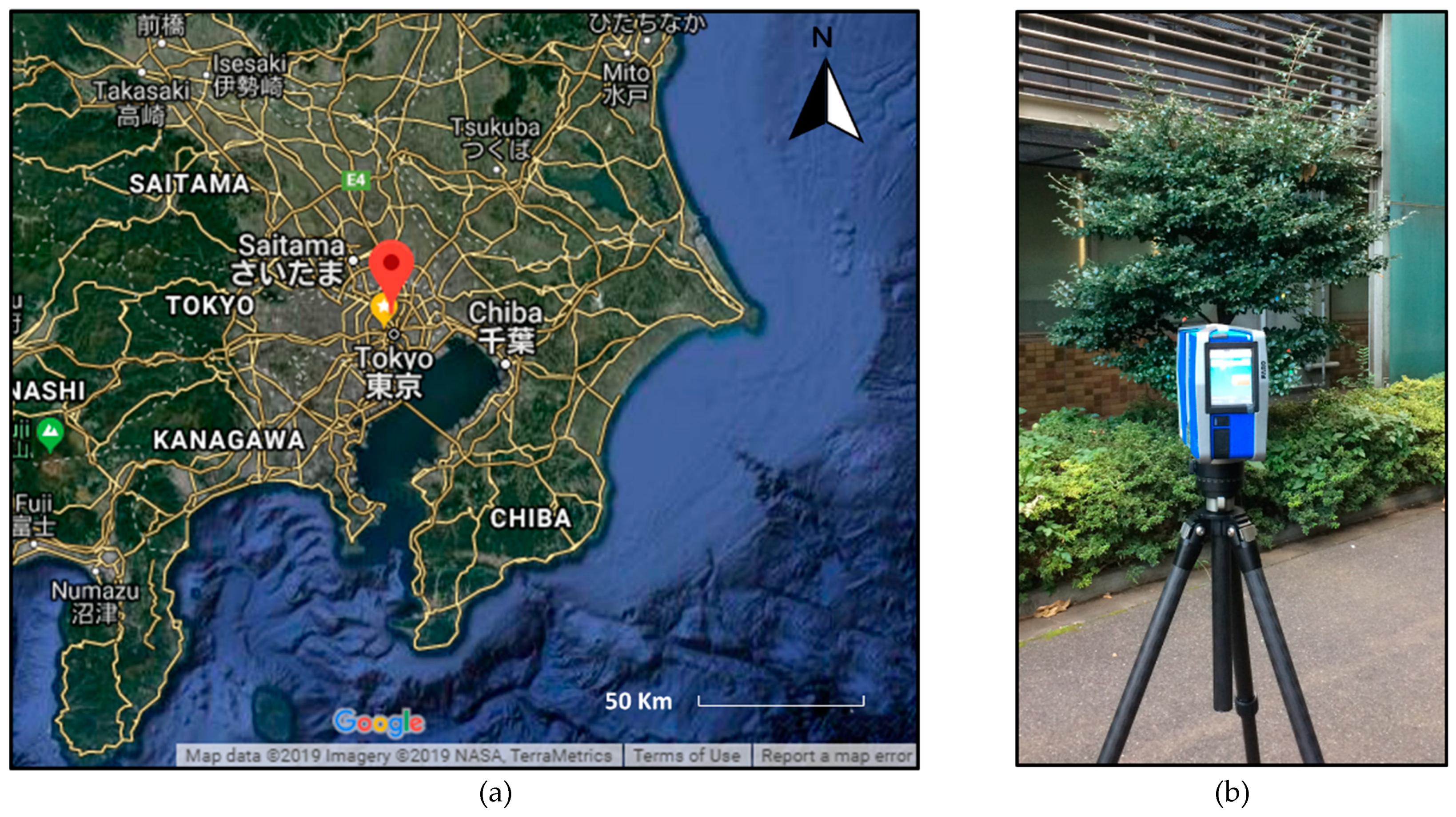
2.1. Study Site and Materials

The terrestrial LiDAR (Light Detection and Ranging) used in this study was a Focus3D X330 (FARO, FL, USA) weighing 5.2 kg with a vertical field of view of 300° and a horizontal field of view of 360°. The measurement speed was 122 to 976 kpts/sec (kpts: thousands of points), with a scan range between 0.6 m and 330 m, a wavelength of 1550 nm, a distance ranging error of ±1 mm, and an angular resolution of 0.009° for each angular scan. The field trial was conducted at the University of Tokyo (Figure 1a), which is located at 35°43’03.1”N 139°45’43.4”E, on 12 November 2018, and the day was windless and sunny. The sampled species included the mochi tree (Ilex integra) and the Japanese camellia (Camellia japonica), which were well isolated and themselves surrounded by the same species. The leaf lengths of the mochi and Japanese camellia tree were approximately 12 and 4 cm, respectively, and the tree heights were 4.5 and 3 m, respectively.

2.2. Data Collection/Preprocessing

The scanner was mounted on a 1.5-m-high tripod and placed 3 m in front of the target (Figure 1b). Before scanning, 10 sampling leaves from both of the species were marked using colored tape. The leaf angle was measured with a protractor for subsequent validation purposes [23,24,25]. In order to prevent unreliable data from being taken from the measurement of the leaf angle, the measurements of leaf angle in each leaf sample were performed cautiously in a windless state and were repeated three times to obtain an average value. Each scanning angular resolution was 0.009, and the scanner spent approximately 15 min completing each scan. After scanning, PCDs were collected, and the target leaf PCD parts were manually extracted using CloudCompare software. Except for the leaf PCDs, the nonphotosynthetic parts, such as wood trunks and branches in the canopy, were pre-deleted by grouping the images based on established classification methods for estimating the leaf angle without effects from untargeted materials [26]. Research studies use either geometric- or intensity-based classification methods to group leaf and wood PCDs, but the methods are slightly complicated in terms of procedures [27,28,29]. In contrast, considering that the recently developed laser scanner had its own digital camera, color information could also be used as a basis for classification. In fact, the color components of wood and leaves are intuitively different; therefore, it is not difficult to distinguish between them and classify them according to color difference.

The digital number (DN) in the RGB channel (for red, blue, green three colors) shows the absolute magnitude of the color component in each channel. However, if only the DN is considered, the classification between wood and leaf PCDs is not always successful. We could not guarantee that the DN of leaves in the green channel would always be higher than that of wood even though the leaves looked greener, because the wood material could maintain a higher “brightness”, resulting in a higher wood DN in the green channel. However, if compared under the same brightness conditions, the DN of the wood PCDs in the green channel is relatively lower than the leaf. Therefore, the DN of the PCDs was rescaled via normalization to allow for a comparison under the same brightness conditions. A simple method of doing this is to obtain the value in the target channel and divide it by the sum of the DNs in the R, G, and B channels [20]. However, in this study, another simple way was proposed to emphasize the comparison in the green channel by converting the RGB color space into an L*a*b* color space (is the color space defined by International Commission on Illumination), which contained three representative values: L* for brightness from black (0) to white (100), a* for green (-) to red (+), and b* for blue (-) to yellow (+). Generally, the leaf is greener, which results in mostly negative a* values in the L*a*b* color space, while the a* value of wood is positive. Thus, a threshold a* value was defined to classify the wood and leaf PCDs by averaging the a* values of randomly selected PCDs. Then, the wood PCDs were removed according to the classification results. The accuracy of removal classification was calculated as given in Reference [27]:

$$Accurac{y}_r=\frac{\mathrm{Tw}+\mathrm{Tl}}{\mathrm{Tw}+\mathrm{Tl}+\mathrm{Fw}+\mathrm{Fl}} .$$

(1)

Here, T_w is the number of points correctly classified as wood, F_w is the number of points incorrectly classified as wood, T_l is the number of points correctly classified as a leaf, and T_w is the number of points incorrectly classified as a leaf.

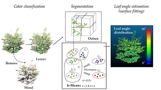
2.3. Leaf Segmentation

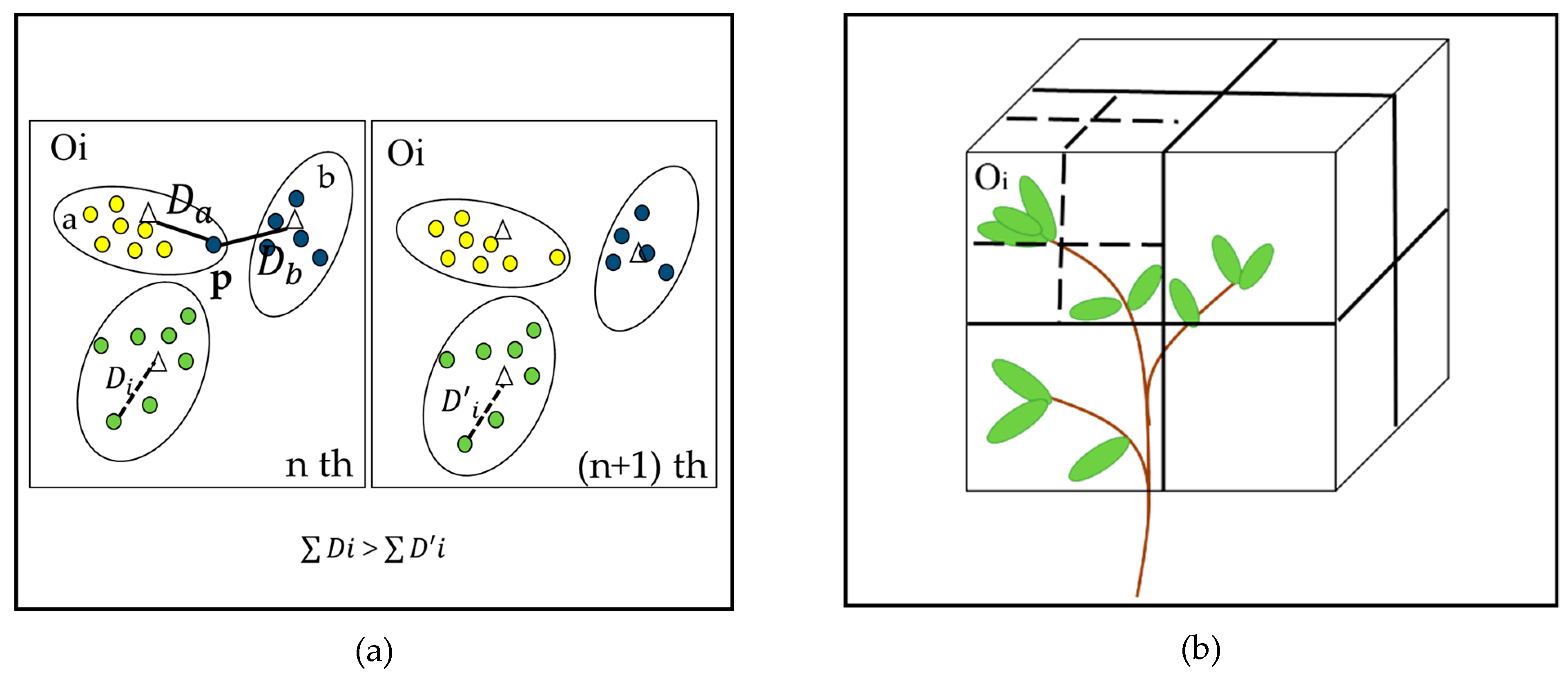
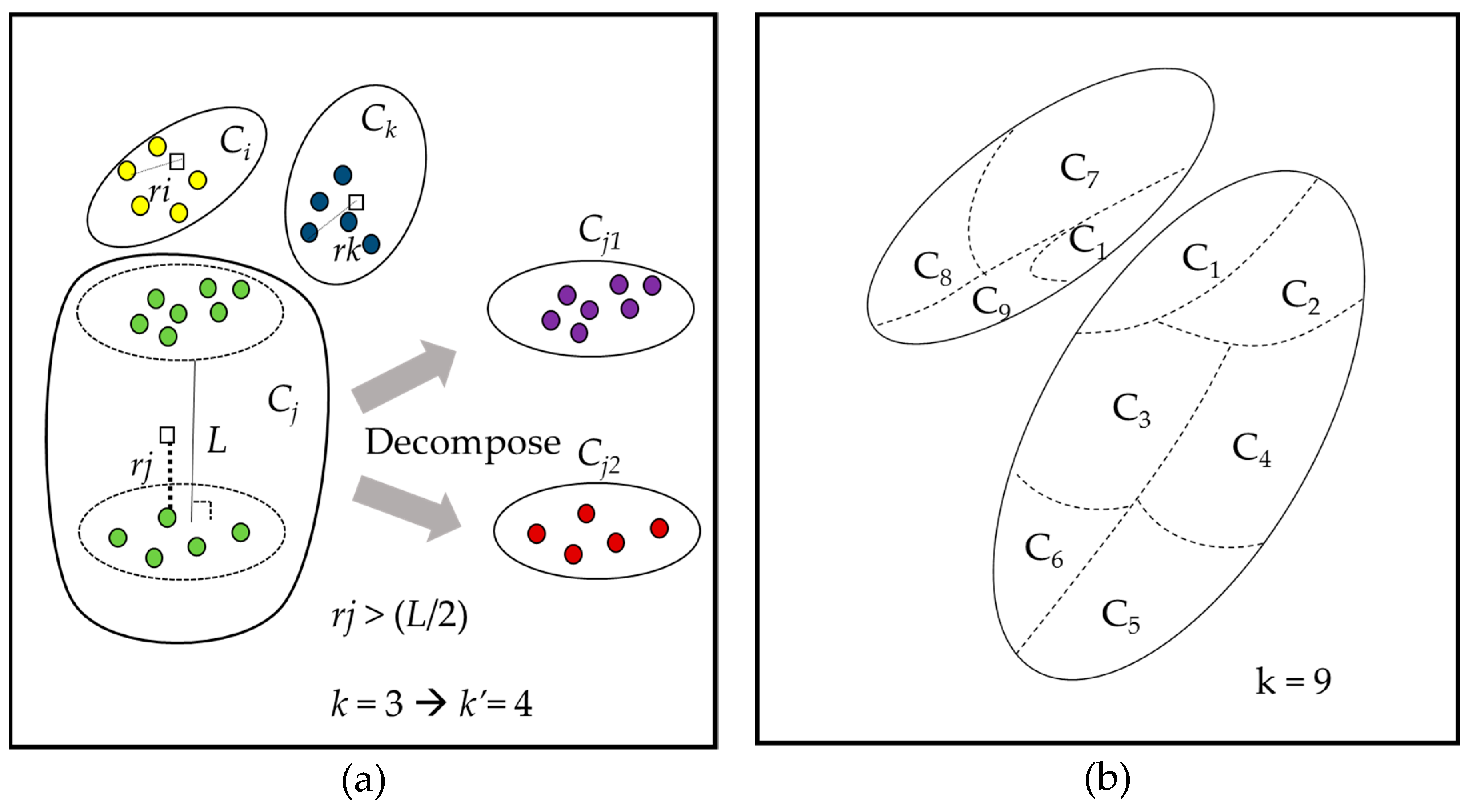
2.3.1. k-Means

The concept of the developed algorithm is demonstrated in the workflow shown in Figure 2. The k-means algorithm has been widely used to group, classify, and segment clusters of point data [30]. This algorithm was used in this study to implement leaf PCD segmentation. The leaf PCDs in a specific region were segmented into small groups, each of which depicted either a single leaf PCD or part of a leaf PCD, based on the initial given parameter k. The parameter k is used for deciding the number of segmentations. Specifying a larger k-value leads to a cluster of PCDs in the space to be segmented into smaller pieces of points groups. The method for deciding the optimal k-value for the k-means algorithm will be discussed later, in Section 2.3.3.

The k-means involves iteratively exploring the centroid of every cluster and then picking and regrouping the near points into a new group. Figure 3a displays the changes in the class boundary and cluster centroid between the nth and (n + 1)th iterations. As shown, in the nth iteration, point p was closer to the centroid of the leaf a. However, it was grouped with leaf b ($D_a<D_b$), which did not lead to the smallest sum of the distance between the points and the cluster’s centroid within the group. Therefore, the leaf PCDs were reorganized to group the p point with leaf a, where ${{\displaystyle \sum }}^{}\mathrm{Di}>{{\displaystyle \sum }}^{}{\mathrm{D}}^{\prime }\mathrm{i}$, and the iteration ended in ${{\displaystyle \sum }}^{}{\mathrm{D}}^{\prime }\mathrm{i}$, which was the smallest. For instance, assuming that ${{\displaystyle \sum }}^{}{\mathrm{D}}^{\prime }\mathrm{i}$ in the (n + 1)th and (n + 2)th iterations were equal, the iteration stopped at the (n + 1)th iteration because the cluster in the (n+1)th iteration was the smallest.

2.3.2. Octree

Use of the k-means algorithm helps in careful segmentation of the PCD clusters, but running the program across all PCDs has limitations of memory and time consumption. For these reasons, the leaf PCDs were spatially discretized into subspaces based on an octree structure [31] to reduce computational complexity and memory usage before running them through the k-means. The octree structure is an effective approach for assigning point clouds to uniform subspaces. On the basis of an octree structure, the leaf PCDs were split into eight subspaces in every iteration until the number of points was less than the specified number (Figure 3b). The number of points in each octree space unit was limited to 1500 in both the sampled species to maintain high computational efficiency for each batch processing of k-means in every octree unit space. Besides, an estimation of the number of leaves in an octree unit is helpful in deciding the initial k-value and reducing unnecessary computation in the k-means algorithm. This number was initially unknown, but the points of a single leaf were counted to approximately estimate the total number of leaves that might be included in an octree unit space. In our case, the average number of points in a single leaf was between 500 and 1500. Therefore, one octree unit space (Oi) was expected to contain 1 to 3 leaves.

2.3.3. k-Value for k-Means

The k-value, which is the initial parameter of the k-means, is the total number of segments expected in the PCDs. The elbow method has been introduced to determine the robustly optimal k-value in the literature [30,32]. However, the insignificant spatial deviation of datasets might occur with different k-values, leading to criticism due to unsuccessful performance. The k-value is expected to be equal to or greater than the number of leaves (N) to prevent multiple leaves from being grouped into the same cluster (k ≧ N). In other words, knowing the value of N explicitly is of great interest in determining the optimal k-value. As discussed previously (Section 2.3.2), N can simply be estimated by evaluating the relationship between the total number of points in a single leaf and the octree unit space. In addition, as described in a previous section, one octree unit space (Oi) is expected to contain 1 to 3 leaves. Therefore, the initial k-value should be set to at least greater than 3 (k ≧ N = 3). However, in reality, the estimation of N is not always correct. In Figure 4a, N is truly equal to 4, but the estimation (N = 3) is intrinsically lower. A larger k-value (k → k’) should be given until k’ ≥ N to properly separate the clusters of leaf PCDs into a specific number of clusters. Increasing the k-value without limitation, regardless of a reduction in the number of PCDs, causes the leaf PCDs to become smaller, rendering them susceptible to noise and anomalies in calculating the leaf angle [10] and making the process computationally inefficient.

In this study, a simple method for deciding the k-value is provided by considering the distance of the points from the centroid and the leaf gap distance (L), i.e., the shortest distance between two close leaves. As shown in Figure 4a, the longest distance from the centroid to a cluster point in each group is r. Thus, for the groups Ci, Cj, and Ck, the longest distances are ri, rj, and ri, respectively, where rj > rk > ri. When multiple leaves are included in the group, such as in Cj, the distance r will be longer than half the distance of the leaf gap (r > L/2). In this case, the k-value can be added to have more domains for grouping the leaf PCDs. As can be seen in group Cj, as more than a single leaf is included in group j, the k-value can be increased to k + 1 (i.e., 4). The cluster is split into two different clusters if r of the cluster exceeds a pre-specified value (L/2). As a result, four domains are created, and two leaves being grouped together can be prevented. In other words, it is not required to increase the k-value indefinitely, but only gradually until all r-values in the domains are not beyond (L/2), which means r = {ri …rn} ≦ (L/2) is satisfied. L was set at 2 cm because it mostly ranged from 2 cm to 5 cm in this study. There was consistent accuracy in the segmentation, justifying the approach.

Segmentation based on this approach was compared to manually extracted leaf segments. Leaf PCDs from four to five regions of the sampled trees were manually divided into several individual leaf segments. Each region consisted of approximately 20–30 leaf segments. Figure 4b shows an example of invalid segmentation. Invalid segmentation of a cluster such as C₁ might affect the estimation of a leaf angle individually as well as the total accumulation of the leaf angle distribution. The impact is evaluated by the accuracy of the segmentation, given by

$$Accurac{y}_s=1-\frac{{{\displaystyle \sum }}^{}\mathrm{Fc}}{{{\displaystyle \sum }}^{}\mathrm{Fc}+{{\displaystyle \sum }}^{}\mathrm{Tc}} .$$

(2)

Here, ${{\displaystyle \sum }}^{}\mathrm{Fc}$ is the number of points in false classes that contain the points from more than a single leaf, while ${{\displaystyle \sum }}^{}\mathrm{Tc}$ is the true class, including only a single leaf. For instance, the accuracy of the segmentation shown in Figure 4b is calculated as 1 – (C₁/ C₁ + C₂ +……+ C₉).

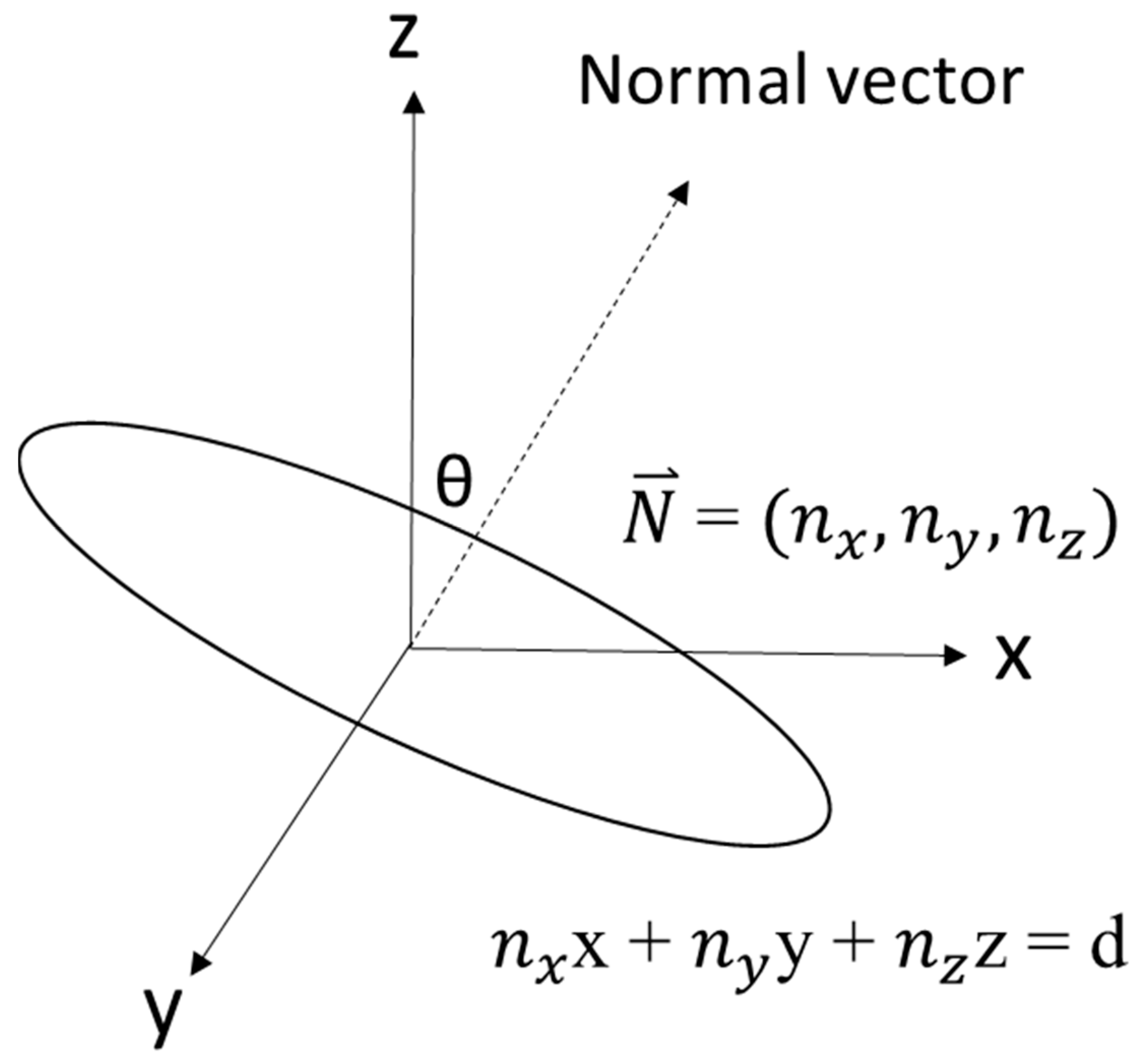
2.4. Leaf Angle Calculation

Definition and Calculation

The leaf angle is defined as the clockwise angle from the zenith (z axis) (shown in Figure 5), which is the angle between the normal vector ($\stackrel{\rightharpoonup }{N}$) and the vector in the z direction.

The leaf angle ${\mathsf{\theta }}_L^{}$ is calculated with respect to the normal vector from the fitted plane ($n_x$x + $n_y$y +$n_z$z = d) of segmented clusters. The following equation is used to calculate the leaf angle. Multiplication by pi/180 is essential to convert units into degrees:

$${\theta }_L^{}=\left(\frac{\pi }{180}\right){\cos }^{-1}\frac{n_z}{|\stackrel{\rightharpoonup }{N}|}$$

(3)

Here, $\stackrel{\rightharpoonup }{N}$ is the normal vector ($n_x,n_{y,}{n}_z$). The normal vector ($\stackrel{\rightharpoonup }{N}$) of the fitted plane was obtained using the least-squares method [26]. The fitted plane has the smallest distance between the plane and the points of clusters. The least-squares method calculates the plane as follows:

$$\mathrm{M}= \frac{1}{n}{\displaystyle \sum }_{i =1}^n(P_i- \overline{P}){(P_i- \overline{P})}^T, P_{i } ϵ P^k.$$

(4)

LAD is commonly proportioned by the number of PCDs, which means that the estimated leaf angle in the region of dense point clouds is likely to dominate the entire computation of LAD. It has been stated that the leaf angle should be weighted by a triangular leaf area for the calculation of the LAD, as the distribution of PCDs is not spatially uniform [10]. However, implementing this is difficult in terms of computational complexity. Instead, the information for calculated leaf angles stored in PCDs was weighted and averaged by cubic cell (0.1 cm) because it was approximately equal to the leaf area. All of the angle values stored in the LAD were calculated with f(θ), as follows:

$$\mathrm{f}\left({\mathsf{\theta }}_j\right)= {\mathsf{\theta }}_j\times N_j/ N.$$

(5)

Here, f(${\mathsf{\theta }}_j$) is a function of the LAD that is used to describe the proportion of the leaf angle in the jth interval (%); ${\mathsf{\theta }}_j$ represents the angle range in the jth interval (5° is assigned at each interval); $N_j$ is the number of cubic cells containing the angle of the jth interval range; and $N$ is the sum of cubic cells in the complete range of intervals.

3. Results and Discussion

3.1. Validation

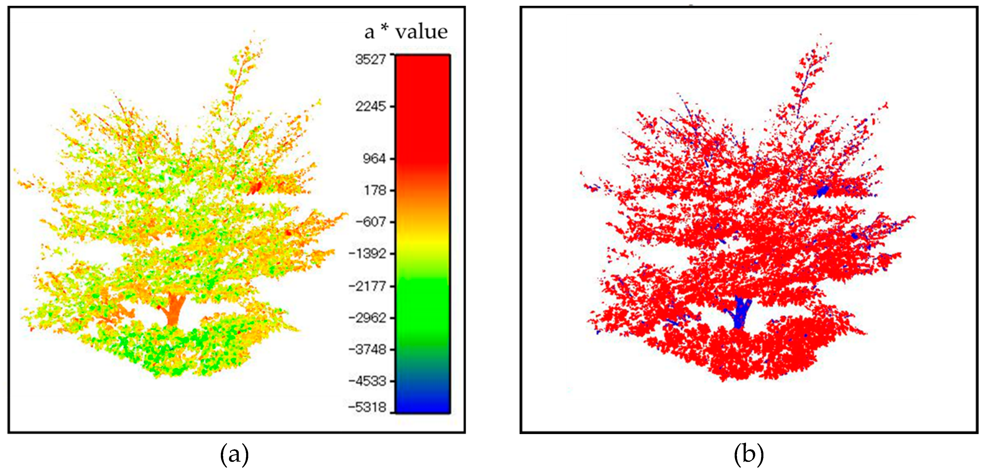
3.1.1. Removal of Non-Photosynthetic Wood

The classification of wood and leaves based on LiDAR-derived PCD geometric features or intensity extractions has been suggested earlier [27,28,29]. In this study, instead of performing complex calculations that were data-dependent, a simple method was adopted based on the difference in color components between the wood and leaves. As a result, the accuracy of classification was 0.93 for the Japanese camellia and 0.91 for the mochi tree, respectively. Figure 6a is a representation of the a* value in the L*a*b* color space after conversion, and the a* value for wood was observed to be higher than for leaves. The classified results are shown in Figure 6b, where the wood is blue and the leaves are red. Our method has the advantage of not requiring any geometric feature extraction calculations and a LiDAR intensity database, but it is limited by its high dependence on lighting conditions. Therefore, it is recommended that these methods be combined according to the situation.

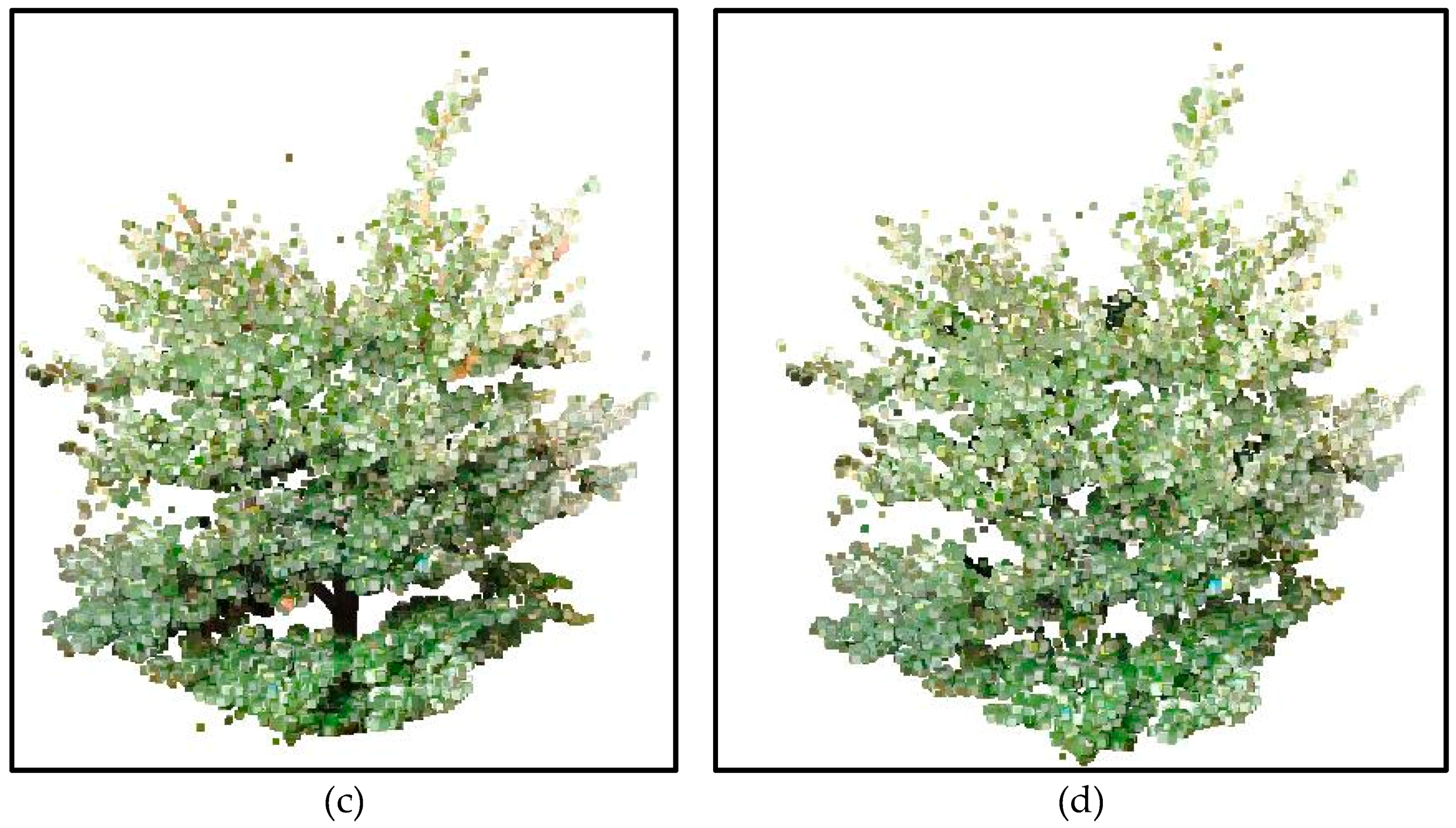
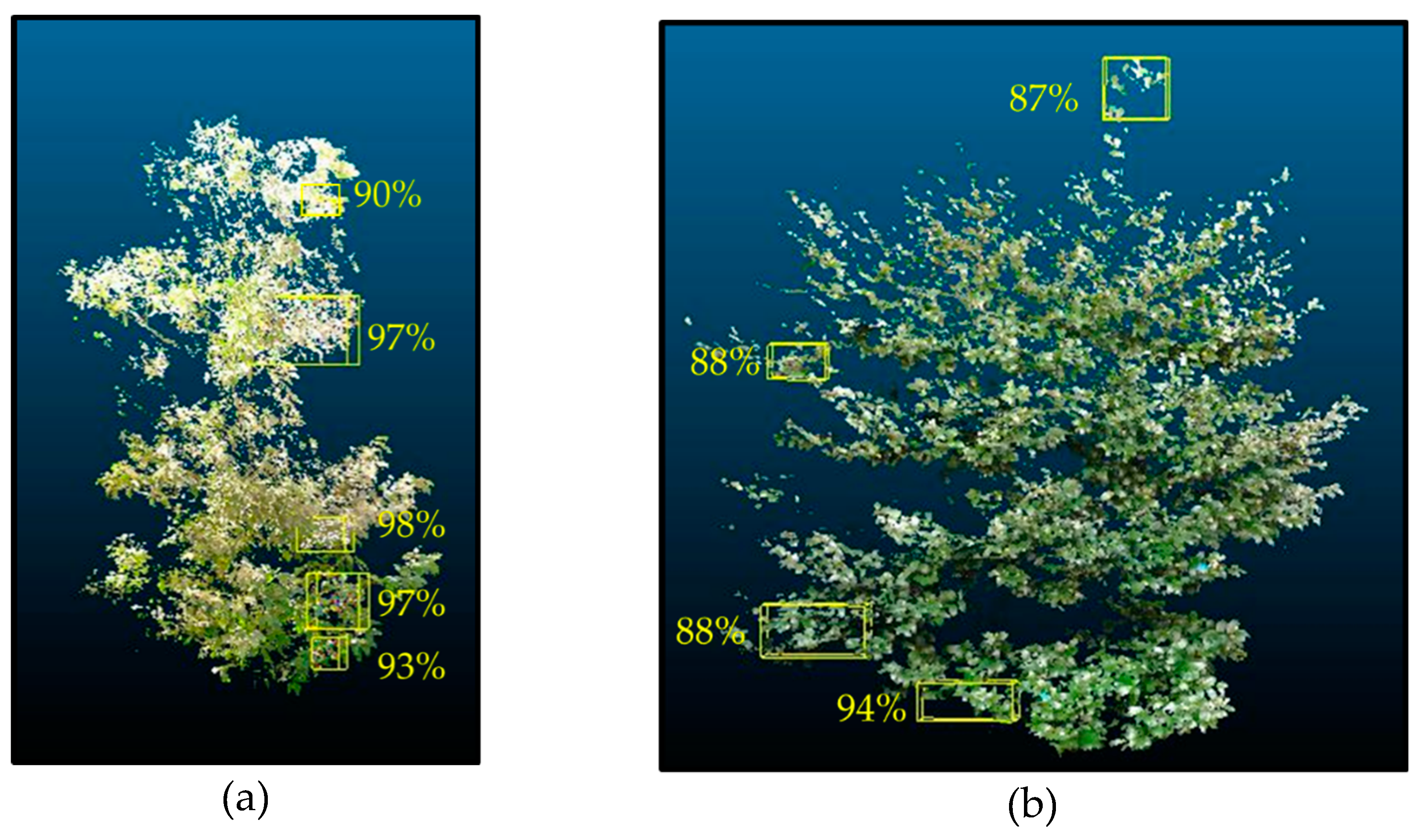
3.1.2. Segmentation of Leaves

The results (Figure 7a,b) showed that our algorithm could segment the leaves with an average accuracy of 95% (ranging from 90% to 98%) for the sampled leaves from the mochi tree and an average accuracy of 90% (ranging from 87% to 94%) for the Japanese camellia. The average classification accuracy for the mochi tree was higher than that for the Japanese camellia. Between the two sampled species, the segmentation accuracy for the top region of the tree was relatively low, and the angular resolution that was degraded over the scanning distance was considered to have a slight influence on the accuracy, but this was not confirmed in the study. Furthermore, the size of the octree space of each terminal node (Oi) may have been the cause of the results. The computational efficiency was considered to be the most affected here. The size of the octree space determined the number of k-values that needed to be specified. When the octree space was large, a larger k-value was required to run k-means, resulting in a longer calculation time. On the one hand, some of the leaves that surrounded the space boundary might have been split into small pieces of incomplete leaves. This might also be a factor affecting the accuracy of classification. Fortunately, our method gradually increases the value of k and can make the value of k eventually larger than the number of clusters in the space. Since the k-value was, finally, greater than the number of clusters in the space, the accuracy of the classification was not affected.

A higher leaf curvature was observed in the Japanese camellia than in the mochi tree, which was caused by the overlapping of leaves. Leaf PCDs of overlapped leaves consist of continuous and close points within the surrounding leaf edges, which makes the group centroid move to a position located in the middle of the leaf gap (Figure 4a, Cj). As the centroid of the grouped cluster is located in the space within the leaves, the distance r (the distance farthest from the centroid, as mentioned earlier, should be specified to be at least less than half of the leaf gap distance to avoid two leaves being classified into the same class (r ≦ L/2). In this case, as the group centroid is positioned in the middle of L, with L assumed at 2 cm, r ≦ 1 cm should be satisfied. Due to the mostly uneven distribution of the PCDs, the group centroid is not located in the middle, but is closer to the leaves, so the condition is satisfied even when the leaf gap is less than 2 cm. However, if the leaf gaps are smaller than 2 cm, for example, 1 cm, and the group centroid is positioned in the middle, the condition must be set at r ≦ 0.5 cm to prevent false segmentation. The lower the value of the required r distance, the larger the k-value to operate the k-means is. Even assuming that a larger k is possible in suppressing the limit, the decreased computational efficiency and the noise effect on the leaf angle estimation of a small group of clusters cannot be ignored (for example, in our case, using the general commercial computers, it took 2–5 min to complete the calculation using a sampled tree formed by about 2 million PCDs). In addition, after the verification of accuracy, the segmentation error was considered to be small enough to affect the estimation of LAD. Therefore, we compromised here by approximating more accurate results while maintaining higher computational efficiency without increasing the k-value.

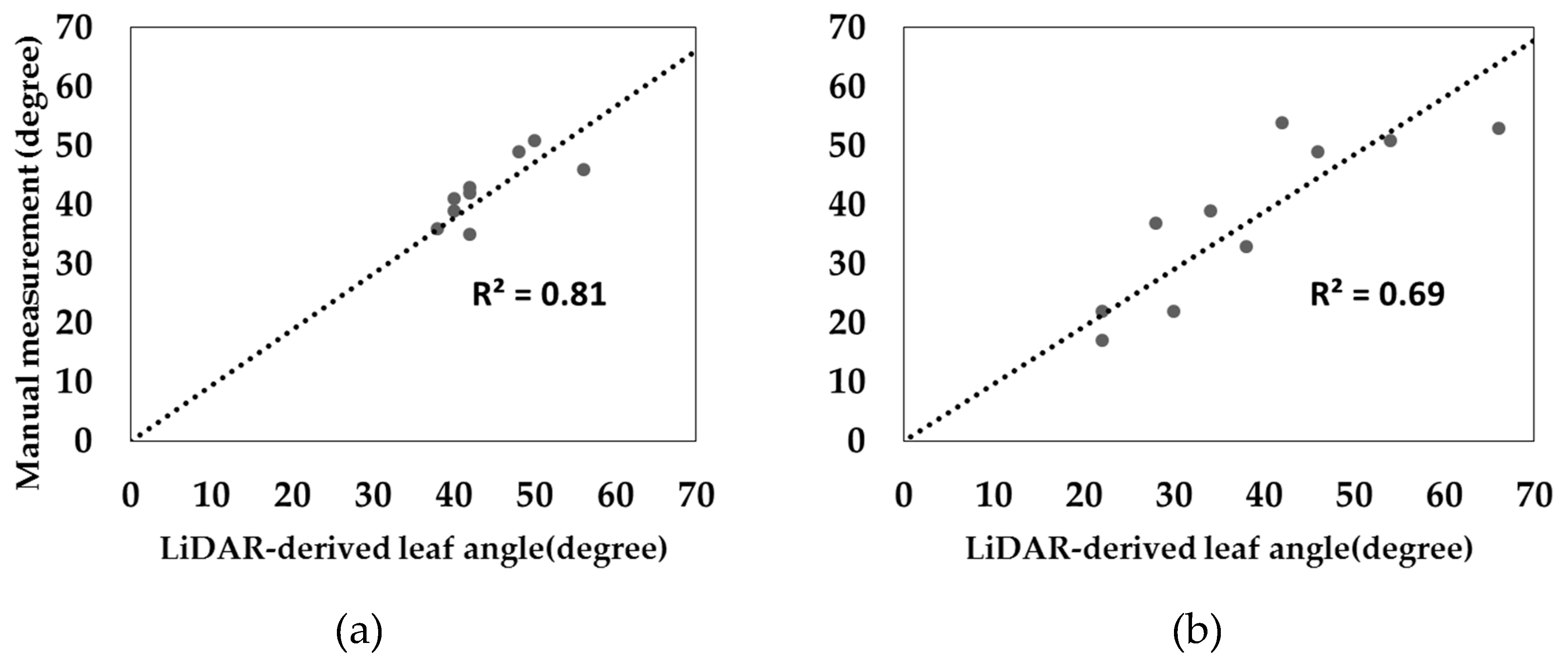
3.1.3. Leaf Angle Estimates Based on Plane-Fitting Method

As is evident from the results shown in Figure 8, the absolute error of leaf angles in the Japanese camellia (6°) was higher than in the mochi tree (3°), which is evident from the R-squared value for the mochi tree (R² = 0.81) and the Japanese camellia tree (R² = 0.69). The average absolute error was higher than the absolute error (2.5°) obtained in Reference [25]. This was because most of the sampling species used in that study had broad leaves that had a lower curvature (flat) and contained less overlapped leaves. In general, the leaf angle estimate based on the fitting surface method is susceptible to surface curvature in the samples. The normal vector used to calculate the leaf angle cannot be accurately estimated in higher-curvature clusters by a single fitted plane [33,34]. More internal leaf segmentation with multiple plane-fittings is required to calculate a more accurate local leaf angle within the leaf. Given this initial condition, r will be less than the specific number specified in the study, and the internal leaf segmentation will have to be split more; in other words, the partition size of segmentation will have to be smaller to make the leaf angle estimation accurate if following the plane-fitting method. However, as described in Section 3.1.2, the computational efficiency and the size of the segmentation area are susceptible to ambient noise. Because such an experiment requires a larger variety of samples, a detailed description of the effect of curvature on determining the k-means is omitted here.

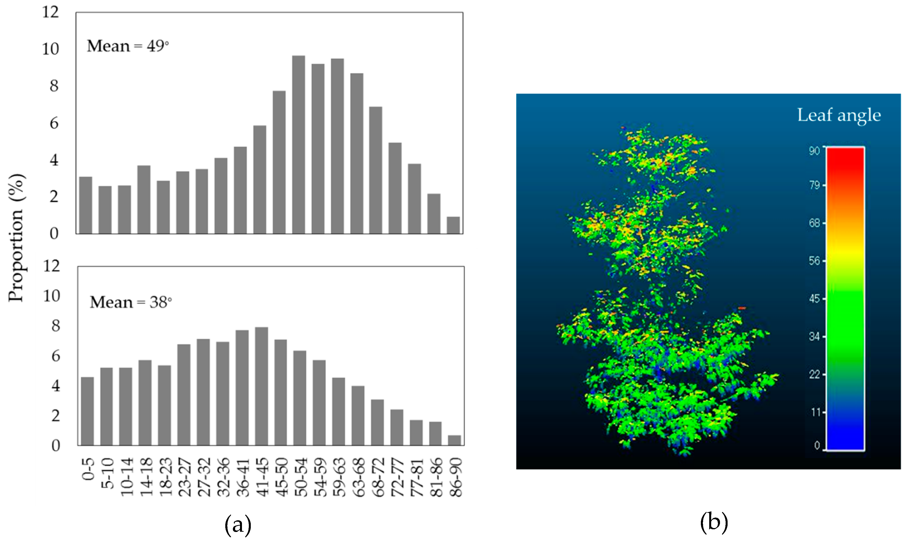
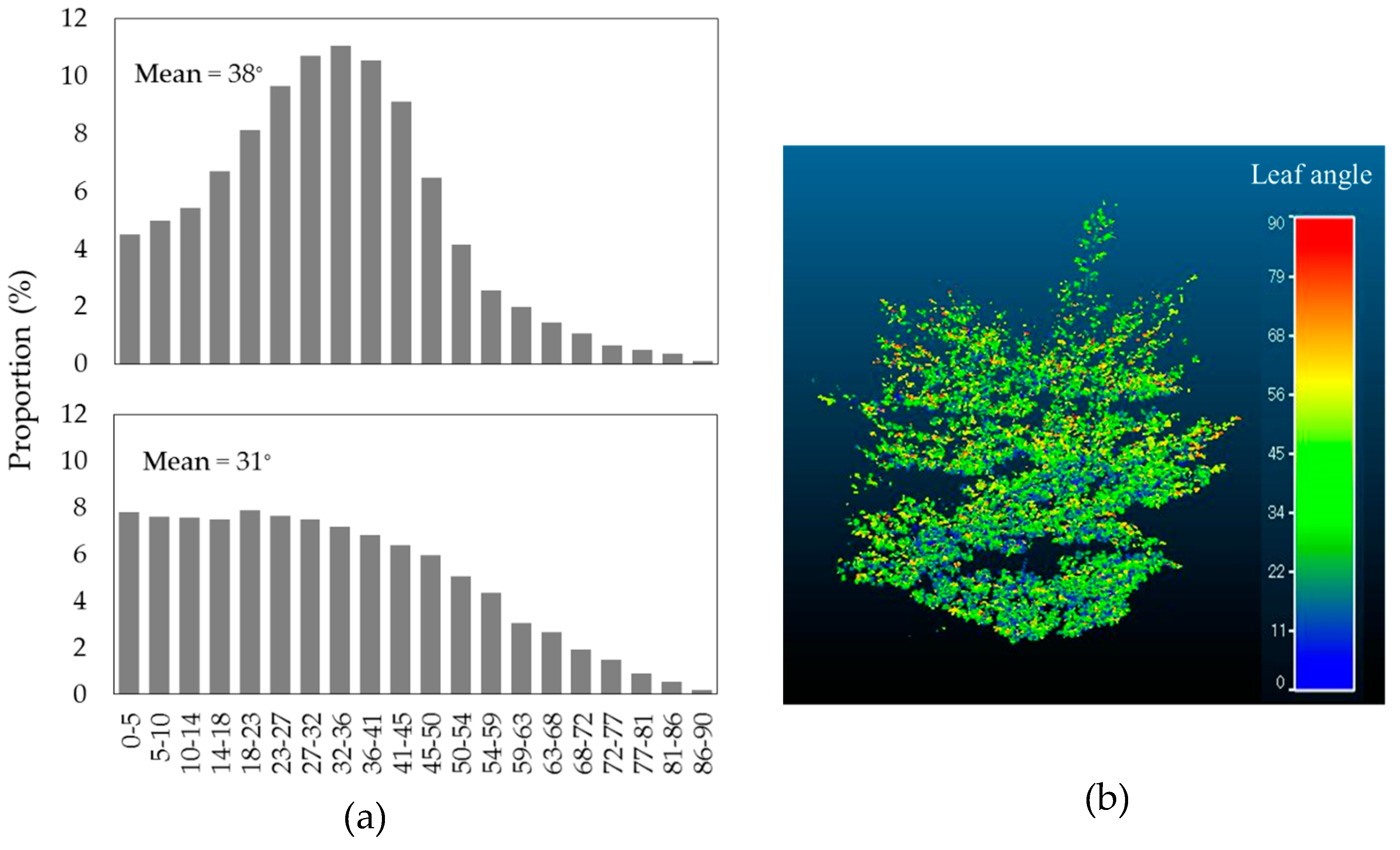
3.2. Leaf Angle Distribution (LAD)

The tendency observed in this study is consistent with other findings where the species maximized the solar interception by changing their LAD [10]. In the mochi tree, the angle of the leaves in the canopy appeared to be mostly inclined at 50° in the higher regions and 32° near the ground (Figure 9). The LAD of the Japanese camellia behaved like the mochi tree, with the leaves inclined horizontally at the top and gradually inclining toward vertical toward the bottom, but the average LAD was more vertical (Figure 10). The LAD in both species revealed that their canopies employed the same concept to effectively use light energy. In agreement with Reference [23], the leaf angle of the species inclined toward horizontal at the top and toward vertical near the ground to increase the leaf outer edge to maximize sunlight interception.

4. Conclusions

In this study, we successfully developed an algorithm to estimate the leaf angle with LiDAR-derived point cloud data. The study focused on an efficient solution for leaf segmentation and estimation of the leaf angle. A leaf segmentation method based on k-means coupled with an octree structure was proposed. In addition, the issue of possible segmentation errors, which has been omitted in the majority of previous studies but which potentially affects the estimation of leaf angle distribution, was discussed. As was shown by the presented results, using our approaches to estimate the leaf angle shows high potential. A strong agreement in the relation and fewer potential errors between the LiDAR-derived and manual measurements were discovered. High leaf curvature within the leaf classification region was considered to affect the accuracy of leaf angle estimation. Fortunately, even if such a problem presents itself, our approach can flexibly change the extent of the size of the classification region based on an automatic adjustment of the k-value to achieve more accurate results. It seems likely that depending on the range of the leaf classification region, the level of effect of leaf curvature on the leaf angle estimation is different, but there was not enough evidence to prove this here. Thus, in future work, we would like to collect data from sampling trees with different curvatures to discuss them for achieving higher leaf angle estimation. Furthermore, due to the location of the target tree, it is difficult to use data from more than one location of LiDAR surrounding the target tree to prevent effect of leaf occlusion on reconstruction of 3D model for LAD estimation. To achieve more accurate results of LAD estimation, future improvements will also focus on field experimental design for data collection.

Looking at our study, automatic classification was achieved by specifying a different initial parameter (L) to find the k-value. We considered that this approach is also possible for other issues related to unsupervised classification. Besides, the LiDAR-derived leaf angle method may also be useful in retrieving another leaf structural parameter, such as the leaf area index (LAI) [35,36]. Aside from the remote sensing field, this method may also prove to be effective in the measurement of the leaf angle distribution in agriculture-relevant fields. A method for accurate leaf inclination estimation in small plants has already been reported [18,36]. The estimation could lead to leaf area estimation and plant structural information monitoring. In combination with our proposed method, we expect that more accurate leaf inclination angle estimation can be accomplished for leaf edges, even in small plants. For these reasons, the presented method has the potential to contribute to various fields, including remote sensing and agriculture.

References

1. Welles, J.M. Some indirect methods of estimating canopy structure. Remote Sens Rev. 1990, 5, 31–43. [Google Scholar] [CrossRef]
2. Falster, D.S.; Westoby, M. Leaf size and angle vary widely across species: What consequences for light interception? New Phytol. 2003, 158, 509–525. [Google Scholar] [CrossRef]
3. Bréda, N.J.J. Ground-based measurements of leaf area index: A review of methods, instruments and current controversies. J. Exp. Bot. 2003, 54, 2403–2417. [Google Scholar] [CrossRef] [PubMed]
4. Ogunbadewa, E.Y. Tracking seasonal changes in vegetation phenology with a SunScan canopy analyzer in northwestern England. For. Sci. Technol. 2012, 8, 161–172. [Google Scholar] [CrossRef]
5. Moorthy, I.; Miller, J.R.; Hu, B.; Chen, J.; Li, Q. Retrieving crown leaf area index from an individual tree using ground-based lidar data. Can. J. Remote Sens. 2008, 34, 320–332. [Google Scholar] [CrossRef]
6. Weiss, M.; Baret, F.; Smith, G.J.; Jonckheere, I.; Coppin, P. Review of methods for in situ leaf area index (LAI) determination Part II. Estimation of LAI, errors and sampling. Agric. For. Meteorol. 2004, 121, 37–53. [Google Scholar] [CrossRef]
7. Goudriaan, J. The bare bones of leaf-angle distribution in radiation models for canopy photosynthesis and energy exchange. Agric. For. Meteorol. 1988, 43, 155–169. [Google Scholar] [CrossRef] [Green Version]
8. Norman, J.M.; Campbell, G.S. Canopy structure. In Plant Physiological Ecology: Field Methods and Instrumentation; Springer: Dordrecht, The Netherlands, 1989; pp. 301–325. [Google Scholar] [CrossRef]
9. Welles, J.M.; Cohen, S. Canopy structure measurement by gap fraction analysis using commercial instrumentation. J. Exp. Bot. 1996, 47, 1335–1342. [Google Scholar] [CrossRef]
10. Bailey, B.N.; Mahaffee, W.F. Rapid measurement of the three-dimensional distribution of leaf orientation and the leaf angle probability density function using terrestrial LiDAR scanning. Remote Sens. Environ. 2017, 194, 63–76. [Google Scholar] [CrossRef] [Green Version]
11. Wang, W.M.; Li, Z.L.; Su, H.B. Comparison of leaf angle distribution functions: Effects on extinction coefficient and fraction of sunlit foliage. Agric. For. Meteorol. 2007, 143, 106–122. [Google Scholar] [CrossRef]
12. Campbell, G.S. Extinction coefficients for radiation in plant canopies calculated using an ellipsoidal inclination angle distribution. Agric. For. Meteorol. 1986, 36, 317–321. [Google Scholar] [CrossRef]
13. Campbell, G.S. Derivation of an angle density function for canopies with ellipsoidal leaf angle distributions. Agric. For. Meteorol. 1990, 49, 173–176. [Google Scholar] [CrossRef]
14. Pisek, J.; Ryu, Y.; Alikas, K. Estimating leaf inclination and G-function from leveled digital camera photography in broadleaf canopies. Trees-Struct. Funct. 2011, 25, 919–924. [Google Scholar] [CrossRef]
15. Müller-Linow, M.; Pinto-Espinosa, F.; Scharr, H.; Rascher, U. The leaf angle distribution of natural plant populations: Assessing the canopy with a novel software tool. Plant Methods 2015, 11, 1–16. [Google Scholar] [CrossRef]
16. Vicari, M.B.; Pisek, J.; Disney, M. New estimates of leaf angle distribution from terrestrial LiDAR: Comparison with measured and modelled estimates from nine broadleaf tree species. Agric. For. Meteorol. 2019, 264, 322–333. [Google Scholar] [CrossRef]
17. Zhao, K.; García, M.; Liu, S.; Guo, Q.; Chen, G.; Zhang, X.; Zhou, Y.; Meng, X. Terrestrial lidar remote sensing of forests: Maximum likelihood estimates of canopy profile, leaf area index, and leaf angle distribution. Agric. For. Meteorol. 2015, 209–210, 100–113. [Google Scholar] [CrossRef]
18. Itakura, K.; Kamakura, I.; Hosoi, F. Three-Dimensional Monitoring of Plant Structural Parameters and Chlorophyll Distribution. Sensors 2019, 19, 413. [Google Scholar] [CrossRef]
19. Zheng, G.; Moskal, L.M. Leaf orientation retrieval from terrestrial laser scanning (TLS) data. IEEE Trans. Geosci. Remote Sens. 2012, 50, 3970–3979. [Google Scholar] [CrossRef]
20. Béland, M.; Widlowski, J.L.; Fournier, R.A.; Côté, J.F.; Verstraete, M.M. Estimating leaf area distribution in savanna trees from terrestrial LiDAR measurements. Agric. For. Meteorol. 2011, 151, 1252–1266. [Google Scholar] [CrossRef]
21. Li, S.; Dai, L.; Wang, H.; Wang, Y.; He, Z.; Lin, S. Estimating Leaf Area Density of Individual Trees Using the Point Cloud Segmentation of Terrestrial LiDAR Data and a Voxel-Based Model. Remote Sens. 2017, 9, 1202. [Google Scholar] [CrossRef]
22. Hosoi, F.; Omasa, K. Factors contributing to accuracy in the estimation of the woody canopy leaf area density profile using 3D portable lidar imaging. J. Exp. Bot. 2007, 58, 3463–3473. [Google Scholar] [CrossRef] [PubMed] [Green Version]
23. Hosoi, F.; Omasa, K. Estimating leaf inclination angle distribution of broad-leaved trees in each part of the canopies by a high-resolution portable scanning lidar. J. Agric. Meteorol. 2015, 71, 136–141. [Google Scholar] [CrossRef] [Green Version]
24. Eitel, J.U.H.; Vierling, L.A.; Long, D.S. Simultaneous measurements of plant structure and chlorophyll content in broadleaf saplings with a terrestrial laser scanner. Remote Sens. Environ. 2010, 114, 2229–2237. [Google Scholar] [CrossRef]
25. Itakura, K.; Hosoi, F. Estimation of leaf inclination angle in three-dimensional plant images obtained from lidar. Remote Sens. 2019, 11, 344. [Google Scholar] [CrossRef]
26. Jin, S.; Tamura, M.; Susaki, J. A new approach to retrieve leaf normal distribution using terrestrial laser scanners. J. For. Res. 2016, 27, 631–638. [Google Scholar] [CrossRef]
27. Tao, S.; Guo, Q.; Xu, S.; Su, Y.; Li, Y.; Wu, F. A geometric method for wood-leaf separation using terrestrial and simulated lidar data. Photogramm. Eng. Remote Sens. 2015, 81, 767–776. [Google Scholar] [CrossRef]
28. Ma, L.; Zheng, G.; Eitel, J.U.H.; Moskal, L.M.; He, W.; Huang, H. Improved Salient Feature-Based Approach for Automatically Separating Photosynthetic and Nonphotosynthetic Components within Terrestrial Lidar Point Cloud Data of Forest Canopies. IEEE Trans. Geosci. Remote Sens. 2016, 54, 679–696. [Google Scholar] [CrossRef]
29. Vicari, M.B.; Disney, M.; Wilkes, P.; Burt, A.; Calders, K.; Woodgate, W. Leaf and wood classification framework for terrestrial LiDAR point clouds. Methods Ecol. Evol. 2019, 10, 680–694. [Google Scholar] [CrossRef] [Green Version]
30. Jain, A.K.; Murty, M.N.; Flynn, P.J. Data clustering: A review. Proc. ACM Comput. Surv. 1999, 31, 264–323. [Google Scholar] [CrossRef]
31. Meagher, D. Octree Encoding: A New Technique for the Representation, Manipulation and Display of Arbitrary 3-D Objects by Computer; Rensselaer Polytechnic Institute: New York, NY, USA, 1980. [Google Scholar]
32. Purnima, B.; Arvind, K. EBK-Means: A Clustering Technique based on Elbow Method and K-Means in WSN. Int. J. Comput. Appl. 2014, 105, 17–24. [Google Scholar]
33. Hoppe, H.; DeRose, T.; Duchamp, T.; McDonald, J.; Stuetzle, W. Surface reconstruction from unorganized points. In Proceedings of the Proceedings of the 19th Annual Conference on Computer Graphics and Interactive Techniques-SIGGRAPH’92; Chicago, IL, USA, 26–31 July 1992, pp. 71–78. [CrossRef]
34. Mitra, N.J.; Nguyen, A.; Guibas, L. Estimating surface normals in noisy point cloud data. Proc. Int. J. Comput. Geom. Appl. 2004, 14, 261–276. [Google Scholar] [CrossRef]
35. Bailey, B.N.; Mahaffee, W.F. Rapid, high-resolution measurement of leaf area and leaf orientation using terrestrial LiDAR scanning data. Meas. Sci. Technol. 2017, 28, 064006. [Google Scholar] [CrossRef]
36. Itakura, K.; Hosoi, F. Voxel-based leaf area estimation from three-dimensional plant images. J. Agric. Meteorol. 2019, 75, 211–216. [Google Scholar] [CrossRef] [Green Version]
Figure 1. (a) Location of study area (red hot spot; source: ©2019 Imagery, ©2019 NASA, TerraMetrics). (b) Set-up of terrestrial LiDAR.
Remotesensing 11 02536 g001
Figure 2. Workflow of leaf angle estimates.
Remotesensing 11 02536 g002
Figure 3. The algorithm for leaf segmentation: (a) k-means, where triangles and squares represent the centroid of grouped clusters. The distance from the centroid to the group points is D i in the nth iteration and D i in the (n + 1)th iteration. As the sum of D i becomes minimum, the iteration will stop or the iteration will continue. (b) Octree (Oi) is an octree space unit that is divided by octree.
Remotesensing 11 02536 g003
Figure 4. The algorithm for leaf segmentation. (a) The relationship between the distance r and the leaf gap distance (L). The k-value increased from 3 to 4 to decompose more segmented pieces to make rj > (L/2). (b) Example of the result of segmentation. C1 represents invalid segmentation.
Remotesensing 11 02536 g004
Figure 5. Illustrated definition of leaf angle (θ).
Remotesensing 11 02536 g005
Figure 6. The classification for removing non-photosynthetic material in the case of Japanese camellia: (a) a* value in L*a*b* color space; (b) classified results (red: leaves; blue: wood); (c) original sampled tree; (d) sampled tree with wood removed.
Remotesensing 11 02536 g006aRemotesensing 11 02536 g006b
Figure 7. Randomly extracted samples for the validation of leaf segmentation in (a) the mochi tree and (b) the Japanese camellia.
Remotesensing 11 02536 g007
Figure 8. Comparison between manual measurement and LiDAR-derived leaf angle for (a) mochi trees and (b) Japanese camellia.
Remotesensing 11 02536 g008
Figure 9. Leaf angle distribution (LAD) in the Japanese camellia: (a) LAD graph for the tree’s top (4.5–2.3 m) and bottom (2.3–0 m); (b) LAD image of the whole tree.
Remotesensing 11 02536 g009
Figure 10. Leaf angle distribution in the mochi tree: (a) LAD graph for the tree’s top (3–1.5 m) and bottom (1.5–0 m); (b) LAD image of the whole tree.
Remotesensing 11 02536 g010