Abstract
Class imbalance is a key issue for the application of deep learning for remote sensing image classification because a model generated by imbalanced samples training has low classification accuracy for minority classes. In this study, an accurate classification approach using the multistage sampling method and deep neural networks was proposed to classify imbalanced data. We first balance samples by multistage sampling to obtain the training sets. Then, a state-of-the-art model is adopted by combining the advantages of atrous spatial pyramid pooling (ASPP) and Encoder-Decoder for pixel-wise classification, which are two different types of fully convolutional networks (FCNs) that can obtain contextual information of multiple levels in the Encoder stage. The details and spatial dimensions of targets are restored using such information during the Decoder stage. We employ four deep learning-based classification algorithms (basic FCN, FCN-8S, ASPP, and Encoder-Decoder with ASPP of our approach) on multistage training sets (original, MUS1, and MUS2) of WorldView-3 images in southeastern Qinghai-Tibet Plateau and GF-2 images in northeastern Beijing for comparison. The experiments show that, compared with existing sets (original, MUS1, and identical) and existing method (cost weighting), the MUS2 training set of multistage sampling significantly enhance the classification performance for minority classes. Our approach shows distinct advantages for imbalanced data.
1. Introduction
Remote sensing technology is an important method of monitoring land cover changes and has been widely used in various fields, including environmental monitoring, urban planning, and military reconnaissance [1,2,3,4]. High-resolution (2 m spatial resolution and higher) remote sensing images can provide more details about the ground objects than low -spatial -resolution (10–30 m) images, as well as a higher diversity of ground targets and complexity of their spatial-temporal distribution.
Traditional classification methods used for low -spatial -resolution images can be divided into unsupervised classification methods, such as k-means [5] and ISODATA [6], and supervised classification methods, such as the maximum likelihood method [7], artificial neural networks [8], support vector machines [9], and random forests [10]. In these methods, pixels are the basic unit of classification, spectral features of representative ground objects are extracted from images, and the similarity of the spectral features are used to determine the classes. Classification accuracy may be low because objects made from the same or similar materials cannot be adequately distinguished using spectral features [11]. Object-oriented image classification methods focus on the objects generated by image segmentation, and both spectral features and spatial features are considered in the classification. Object-oriented image classification methods are not subject to the deficiencies of pixel-level classification methods, and have been widely applied in high-resolution image classification [12,13].
The complexity of surface targets in remote sensing images and the influence of multiple factors (noise, season, sunlight, and human activity) pose tremendous difficulties for high-resolution image classification. It is still difficult to obtain accurate classification, even using object-oriented classification methods [14]. Excellent feature expression is crucial for ensuring the accuracy of classification algorithms, but feature extraction is primarily performed manually and often depends on experience. Sebastian [15] discussed and analyzed selection of classification models subject to the conditions of the dataset, expectation result, and hardware condition. From the perspective of application, our goal is image classification with large areas that have uneven distribution of ground objects distribution, and we have ready-made images and corresponding ground truth labels. Automatic and accurate intelligent classification is of greater practical value, with respect to object-oriented image classification methods with support vector machines (SVM) classifier that extract effective features.
Deep learning achieved state-of-the-art performance in natural image semantic segmentation, and it has been widely used in intelligent analysis [16,17]. Therefore, deep-learning-based high-resolution remote sensing image classification is of great significance because of the large amount of information in these images [18]. The convolutional neural network (CNN) developed by LeCun et al. [19] was the first learning algorithm with a truly multilayered structure. The network structure can be optimized by making full use of the locality of the data based on local sensing, weight sharing, and spatial pooling. Displacement and deformation invariance are also ensured to some extent. Therefore, it exhibits a higher classification accuracy with a lower error rate than traditional image classification methods [20,21]. The two-dimensional image structure is not preserved by CNNs because one image output corresponds to only one class label. However, the output of a dense class map is usually required for high-resolution remote sensing image classification, and the class label distribution of class map must correspond to the pixels. In the fully convolutional network (FCN) proposed by Long et al. [22], the two-dimensional image structure is maintained by replacing the last several fully connected layers in the standard CNN with convolutional layers. In addition, images of any sizes can be the input, and the one-to-one correspondence between predicted class labels and original pixel elements is established, thereby realizing pixel-level classification. To address pixel-level dense image prediction, Yu [23] developed a new atrous convolution network module that was able to systematically gather multiscale contextual information without losing resolution. In a study by Zheng et al. [24], end-to-end classification was implemented by embedding the solution process of conditional random fields (CRFs) into a recurrent neural network (RNN) model during training. A deepLab framework of atrous convolution with post -processing by CRF was proposed by Chen et al. [25]. The receptive field could be expanded by atrous convolution when the calculated amount remained unchanged. The edge of the classification result was strengthened by the CRF. Later in 2017, the same group proposed atrous spatial pyramid pooling (ASPP) [26,27] where the output features were combined through multiple parallel atrous convolutions of various sampling rates integrating multiscale information. Furthermore, a Decoder module was added, and the multiscale features from the Encoder stage were used in the Decoder stage to restore the spatial resolution [28]. With ASPP, the classification result could be improved without optimization by CRF post-processing [29].
Deep learning has achieved high accuracy in high-resolution remote sensing image classification [30]. Volpi [31] presented a CNN-based system relying on a downsample-upsample architecture, which could learn to densely label every pixel at the original resolution of the image. Lagkvist et al. [32] applied a CNN to the multispectral orthorectified imaging and digital surface model (DSM) of small-sized cities to realize complete, rapid, and accurate pixel-level classification. Compared with other pixel-level classification methods, this method was more accurate. Fu et al. [14] designed a multi-scale network architecture with a high classification accuracy of 81% by adding a skip-layer structure to the multi-resolution image classification of GF-2 images and IKONOS true color images. A CNN model pretrained on ImageNet was developed by Marmanis [33] to address other, different classification issues. The overall accuracy of this model on the UC Merced Land Use benchmark [34] was increased to 92.4%. Maggiori et al. [35] proposed an end-to-end framework for the dense pixel-wise classification of large-scale remote sensing images with CNNs, which provides fine-grained classification maps by taking a large amount of contextual information into account. Kampffmeyer et al. [36] combined the variants of two neural networks based on the deep learning network model, and the classification performance was improved for small-objects. Kussul [37] described a CNN architecture that outperformed the existing methods. It included an ensemble of multilayer perceptrons (MLPs) and a random forest (RF) classifier with accuracy levels of more than 85% for all major crops. Wang et al. [38] proposed an efficient model by combining ASPP and Decoder for dense semantics on the Potsdam and Vaihingen datasets. Compared with DeepLab_v3+, the model gains 0.4% and 0.6% improvements in overall accuracy on the two datasets respectively.
The Qinghai-Tibet Plateau is mainly a depopulated region characterized by great variability in ground object areas, complex shapes, uneven distributions of ground objects, and small sizes of targets. It may lead to pixel scales of different ground object classes on the high-resolution remote sensing images differing widely. We created Worldview-3 image labeling dataset, and the imbalanced data were used for classification with deep neural networks. A severe imbalance of training samples may emerge in deep learning network models during the training process. The weight of each pixel is considered uniformly distributed by the default in the loss function of the CNN, biased training models may exist in the majority classes with larger proportions in the image, and the minority classes with smaller proportions may also be neglected. This finally results in a poor performance of minority classes in classifying targets, and it causes diminished accuracy for new data [39].
Solutions to sample imbalance primarily include modifying the classifier algorithm and changing the sample set [40,41]. The former is performed by strengthening the ability of the algorithm to learn minority classes. By the comparative study of two approaches for unmanned aerial vehicle (UAV) emergency landing site surface type estimation by Ayhan [42], it is concluded that SVM is less sensitive to imbalanced data. At the same time, the excellent feature expression is crucial for ensuring the accuracy of SVM classifier, which needs manually performed extraction and often depends on experience. A commonly used method is cost-sensitive learning. Cost-sensitive methods assign different misclassification costs for different classes, generally a high cost for the minority class and a low cost for the majority class [43]. Weights of the minority classes are increased by loss weighting. To change the sample set, minority classes are emphasized through random sampling to balance the distribution of various target classes in the sample sets [44], including random over-sampling [45], random under-sampling [46], and hybrid sampling combining the previous two. Galar et al. [47] studied cost-sensitive methods and sampling techniques of the ensemble classifier in binary classification problems, and the results indicated that random under-sampling with ensemble classifier improved the classification performance. The adaptive synthetic (ADASYN) sampling approach for learning from imbalanced datasets proposed by He and Garcia [48] enhanced the accuracy and robustness of learning. A new inverse under-sampling (IRUS) method was developed by Tahir [49], which enhanced the classification performance for 22 UCI datasets. These methods for handling sample imbalance have been widely used in machine-learning classification [50,51,52,53].
To overcome the data imbalance in the southeastern Qinghai-Tibet Plateau, an improved pixel-level high-resolution remote sensing image classification approach was proposed in this study. Training sample sets with more balanced distribution were obtained from the Worldview-3 image labeling dataset by means of multistage sampling. In this study, we defined and investigated two sampling distribution models that (i) are more of a combinatorial nature and easier to compute, and (ii) have solid theoretical justifications, and, hence, a closely approximate contribution to training of the samples including MUS1 and MUS2. Both the training and testing sets were input into the network model Encoder-Decoder with ASPP for training and prediction based on the process presented by Chen [29]. We also adopted the same approach on GF-2 high-resolution remote sensing images of northeastern Beijing for classification to test the validation. The GF-2 dataset presented significantly imbalanced distribution of samples over urban area.
The comparison process was carried out in two parts: (1) comparing the classification accuracies of object-oriented approach (MF-SVM) and four deep-learning-based end-to-end classification network models (basic FCN, FCN-8S, ASPP, and the proposed Encoder-Decoder with ASPP) in the context of different proportional distributions of training samples (original, MUS1, and MUS2) in the study area and evaluating their classification performance; (2) comparing the influence of our approach and existing approaches on the final classification result. For imbalanced data, the result shows that our approach with MUS2 set achieves higher overall accuracy and improves the classification accuracy for minority class.
The remainder of this paper is organized as follows. Section 2 gives an overview of methods to address the problem of high-resolution remote sensing imagery classification of imbalanced data. In Section 3 we describe the experimental setup and results. It provides details about imbalanced datasets, sampling methods, and metrics used for evaluation. Section 4 is the discussion of our method. Finally, Section 5 concludes the whole study.
2. Methods
Image classification for imbalanced data was divided into three stages: data preparation, training, and classification (Figure 1). In the data-preparation stage (Figure 1a), the image data and labeled data, with pixel-class correspondence, were first processed to generate small patches that contain potential ground objects by using superpixel segmentation. Then, multistage sampling was carried out to ensure that the sample proportions of various classes were relatively balanced. The multistage sampling proceeds in two stages called MUS1 and MUS2, representing two totally different sampling ratios between samples of all the classes.
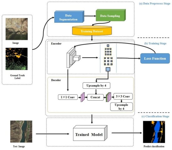
Figure 1.
Workflow of our approach.
In the training stage, image and label data of the MUS1 and MUS2 datasets were input to the network of Encoder-Decoder with ASPP [29] as training samples, respectively (Figure 1b). The output of the network was the predicted class distribution. Cross entropy between the predicted class labels and ground truth (GT) labels was calculated and back-propagated through the network using the chain rule, and then stochastic gradient descent (SGD) with momentum was used to update network parameters.
The test image data were put into the trained network model Encoder-Decoder with ASPP to generate the classification result in the classification stage (Figure 1c).
In the following sections, we present data-segmentation processing using a superpixel algorithm, the proposed multistage sampling method including two sampling ratios between samples from all classes, and explain the use of Encoder-Decoder with ASPP network for pixel-level classification image classification. Weighting loss to address the imbalance of training dataset is finally introduced.
2.1. Data Segmentation
A simple linear iterative clustering (SLIC) algorithm was used for the superpixel segmentation of the images and corresponding label data, thereby generating a complete object, on the basis of which an intact image was segmented into small image blocks to establish the sample dataset (Figure 2). Initially, the gradient values of all the pixels in the neighborhood were calculated, and the seed points were moved to the locations with the smallest gradients. Each pixel was allocated with a class label (indicating the cluster center it belonged to) in the neighborhood of each seed point. The search range of the SLIC was confined to . The distance measurement primarily included color and spatial distances. The distances between each pixel of the search and seed point were calculated using the following equations:
where and are color and spatial distances, respectively, and is the intra-class maximum spatial distance that was applied to every cluster, denoted as . The maximum color distance varied in different images and clusters. Therefore, a constant ([1,40]; usually set to 10) was used as a substitute. The distance could be calculated by
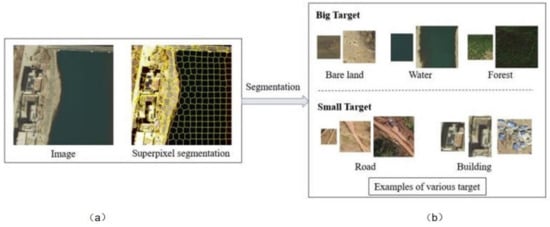
Figure 2.
(a) The original image; (b) The segmented image after superpixel segmentation.
Because every pixel could be searched by multiple seed points, the seed point with the minimum distance to the pixel was taken as the cluster center of the pixel.
2.2. Sampling
2.2.1. Hybrid Sampling
Random over-sampling (Figure 3a) increases the number of samples in minority classes by replicating and generating new samples so that the number matches the majority classes. Here, data augmentation techniques were applied in the data space of minority classes to obtain new samples from existing data. Specifically, new samples were generated by means of translation, rotation, mirroring, scaling, and spatial switching of the color, as well as by adding disturbances. Over-sampling should be applied to the level that completely eliminates the imbalance. It undertakes a balancing of the training dataset by simply reproducing samples from minority classes. However, having replicated similar samples may cause the problem of overfitting especially for minority classes as new samples do not expand the borders of the decision area [54]. As we repeat a small number of samples multiple times, the trained model fits them too well. In addition, both the computational complexity and cost are also increasing.
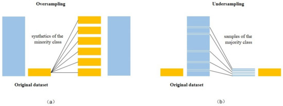
Figure 3.
Random (a) over-sampling (b) under-sampling.
A more advanced sampling method proposed by Chawla that aims to overcome overfitting is synthetic minority oversampling technique (SMOTE) [55]. It creates synthetic minority class examples by interpolating neighboring data points, instead of replicating samples from these classes. Synthetic samples are generated by considering the over-sampling index (the k nearest neighbors) from the same minority class, and interpolating new samples somewhere along the connecting lines between them. SMOTE over-sampling provides more related minority class samples for training, thus strengthening the ability of the classifier to learn minority classes. The existing over-sampling methods based on SMOTE may achieve slightly better than the original one. One of the reasons is that when SMOTE is applied to an extremely skewed dataset, examples generated far from the borderline may contribute little to classification, and its empty feature space is too huge to estimate proper borderlines between classes for classification algorithms.
Under-sampling involves randomly selecting only some of the samples from each majority class to match the minority classes, which reduces the size and training time to some extent, but may cause information loss. Under-sampling showed a generally poor performance. In a large number of analyzed scenarios, under sampling showed decrease in performance as compared to the original dataset [39]. Considering that the final classification accuracy might be affected by the samples from different parts of majority classes, especially those with similar features, random under-sampling (Figure 3b) was used in this study. Instead of discarding a fraction of the samples at random, a rule was set to divide the data into batches. Samples were randomly selected from each batch of data and included in the sample set.
For an extreme ratio of imbalance and large portion of classes being minority ones, under-sampling performs on a par with over-sampling. If training time is an issue, under-sampling is a better choice in such a scenario, because it dramatically reduces the size of the training set. Importantly, we focused on methods that are widely used and relatively feasible to implement as our aim is to draw conclusions that will be practical and serve as guidance to a large number of deep learning researchers and engineers.
Based on our review of the literature [54], in order to avoid the common problems of applying under-sampling and over-sampling separately, hybrid sampling (combination of random over- and under-sampling) is also considered with the purpose of improving the classification performance. For the condition of skewed data, we have gradually decreased the imbalance with hybrid sampling in terms of performance and generalization. Minority class enhancement was used to balance the distribution of training data and reduce the bias of the classifier towards the majority classes.
Even though the datasets were significantly imbalanced, identical sampling can simply rebalance the datasets by taking constant numbers of samples from different classes using hybrid sampling. An example of an identical sampling dataset with 5 classes was presented in Figure 4a. Figure 4a also showed the sample proportions for the other three sampling schema (random under-sampling, random over-sampling, and SMOTE over-sampling) for the same dataset.
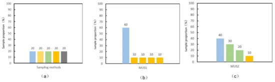
Figure 4.
Example proportional distribution of five sampling schema. (a) sampling method including random under-sampling, random over-sampling, synthetic minority oversampling technique (SMOTE) over-sampling and identical sampling dataset with five classes, (b) multistage sampling dataset MUS1 and (c) multistage sampling dataset MUS2 ().
However, the number of samples from different classes being equal did not always correspond to the optimal results (especially when the class ratio of the minority: majority was extremely skewed) [44]. Therefore, different imbalance ratios between samples of all the classes were considered in the hybrid sampling method.
2.2.2. Multistage Sampling
Different balance ratios between samples from all classes should be taken into account in order to achieve the optimal outcome, while little systematic analysis of hybrid sampling to deal with the deep-learning model is available. In our method for extreme ratios of imbalanced data, we investigated the impact of distribution of samples over different object classes on classification performance of deep neural networks in analytical and quantitative depth, and used hybrid sampling to obtain the optimal sampling ratios between samples of all the classes.
In most multiclass classification of imbalanced data with extreme ratios, only one or two classes might be under-represented or over-represented of original labeling dataset. In this study, we perform multistage sampling on high spatial resolution remote sensing imagery with Multiclass. This is an approach that combines multiple sampling techniques from one or both of the abovementioned categories.
The increasing ratio of examples between majority and minority classes as well as the number of minority classes had a negative effect on performance of the resulting classifiers [39]. We define two stages of hybrid sampling that effectively relieve severe imbalance of training samples, which is the key issue of a wider range of remote sensing satellite imbalanced data.
The first stage of the sampling dataset is MUS1. In the MUS1 set, the sample proportions are equal within minority classes and equal within majority classes by hybrid sampling, and then other classes between the majority and minority do not exist. We apply three expressions to characterize our method.
where N is the total number of classes, and is a set of the examples in class . The other parameter is a ratio between the sample proportion in majority classes and the sample proportion in minority classes.
An example of the MUS1 dataset with a total of five classes, where the parameter , and, more classes being of minority type, was presented in Figure 4b.
After the first stage, the second stage is applied to obtain the MUS2 dataset that has smaller imbalance ratio. We repeat the hybrid sampling process to make the sample proportions in the multiple classes able to be interpolated linearly. The difference between consecutive pairs of classes is of constant order by the value of sample proportion. The constant was defined by the following equation, and we used it in MUS2 as listed.
Which is an example of the MUS2 dataset with four classes, when Figure 4c showed the sample proportion distribution.
2.3. Network Architecture
2.3.1. Fully Convolutional Network
There were several convolutional layers before each down-sampling layer in the FCN. The last layer of the output image was the feature image with three different methods of feature fusion. In the prediction layer, the method for up sampling stride 32 of the conv7 feature map was named FCN-32s (Basic FCN). FCN-16s is a process in which the feature map in the last layer is up sampled of factor 2 and the result is fused with the pool4 feature map and upsampled by a factor 16. In the FCN-8s method, the feature image of FCN-16s is upsampled by a factor 2; the result is fused with pool3 feature map and then up samples of factor 8 [22]. High resolution shallow features that contained detail information were obtained by the front and middle parts of the FCN model. With the deepening of the network, the back part obtained abstract semantic features and interpreted the semantic meaning of each pixel. There were five 2 × 2 down-sampling layers in the FCN. The resolution of an image decreased as it passed through the downsampling layers. Thus, the feature image output from the convolutional layer at the bottom appeared with low resolutions and no clear detail features. If the feature images received FCN-32s directly, the prediction accuracy of some image details would not be high enough; there would also be high edge roughness. With FCN-8s, the location information could be more accurately determined by means of the information in the third and fourth layers of the visual geometry group (VGG) model. The structural diagrams of the different methods were shown in Figure 5.
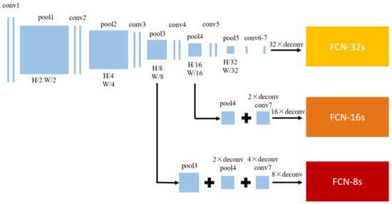
Figure 5.
Fully convolutional network model.
2.3.2. Atrous Convolution for Dense Feature Extraction
Atrous convolution significantly increases the density of the convolutional features. For a given one-dimensional input signal x[i], the size of the convolution kernel is w, and the output of the atrous convolution is y[i], the density can be calculated as follows:
where r is the proportion parameter of the atrous convolution that represents the interval of the convolution operation. The convolution is standard when r = 1. Atrous convolution can play a role in increasing the density of the feature image. As shown in Figure 6, the original images are first downsampled by 1/2 in the simulation of the standard convolution (the red path in Figure 6). Next, the downsampling result underwent a 10 × 10 standard convolution, which was used to simulate the effect of the convolution-pooled sampling in the CNN model. The output feature image was correlated with only 1/4 of the pixel positions of the original image. As a comparison, the atrous convolution (the blue path in Figure 6) was conducted directly on the standard convolution kernel with r = 2 for the original image. The output feature image was correlated with 1/2 of the pixel positions of the original image. With the receptive field kept unchanged, the density of the feature image generated tripled. Compared with the standard convolution, feature images of different resolutions could be generated using the atrous convolution without increasing the number of variables and changing the perceptive field. Furthermore, the perceptive field could be expanded without sacrificing the resolution of the feature space, thereby ensuring the accuracy of the output predictive label map of the CNN.
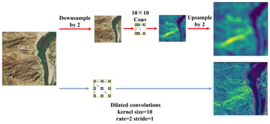
Figure 6.
Diagram of high-density features using atrous convolution.
2.3.3. Atrous Spatial Pyramid Pooling (ASPP)
The last block in the ResNet network (i.e., block 4 of ResNet) is replicated in parallel by ASPP network. There were three 3 × 3 convolutions in each block. Except for the last block, all the other blocks have a convolution stride of 2, and the convolution applies different atrous rates. Following block 4, the final feature image is generated using four parallel atrous convolutions (one 1 × 1 convolution and three 3 × 3 convolutions at expansion rates of 6, 12, and 18). Global average pooling is applied to the feature image to include global contextual information into the model and generate a 1 × 1 convolution kernel with 256 filters. Finally, the features are elevated to a required spatial dimension by means of bilinear interpolation. The network structure is shown in Figure 7.
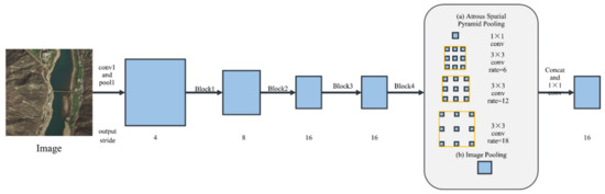
Figure 7.
Network structure of atrous spatial pyramid pooling (ASPP).
The advantage of ASPP was the different sampling rates of the atrous convolutions. Resolution loss could be reduced without increasing the numbers of parameters and amount calculation [26]. This architecture can extract multi-scale features. The ability to extract dense features was strengthened using the atrous convolution. Due to pooling layers and convolutional layer with stride, this method may cause severe loss of boundary information of segmentation targets.
2.3.4. Encoder-Decoder with ASPP
The last feature layer of the ASPP model that contained 256 channels and rich semantic information was taken as the encoder output by the Encoder-Decoder with ASPP. In the decoder, the encoder features are first bilinearly upsampled by a factor of 4, F1, was fused with F2, the result of 1 × 1 convolution (to reduce the number of channels to 48) of the low-level features extracted from the encoder with the same spatial resolution as F1 (the second convolution of block 2). The fusion result, F3, underwent a routine fine-tuned convolution, followed by another simple bilinear upsampling by a factor of 4 to obtain the segmentation result (Figure 8).
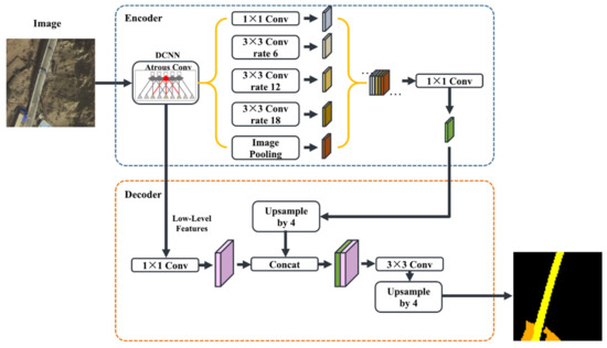
Figure 8.
Network structure of Encoder-Decoder with ASPP.
Cross-entropy loss was used as the loss function of the model:
where , b, , and are the jth weight of the ith neuron, bias, ith output of the network, and actual classification result, respectively; is the output value of softmax, which corresponded to the prediction value of each pixel; and was the true classification result, which was the label value of the pixel point. Dropout was added during training to randomly deactivate some hidden-layer nodes during training to reduce the number of iterating parameters during training and prevent overfitting.
During model training, parameter updating was conducted using stochastic gradient descent (SGD):
where and are the original and updated parameters, respectively; is the parameter increment in the current iteration, which is the combination of the original parameter, gradient, and historical increment:
where is the cost function; is the preset learning-rate parameter used to control the iteration step length; and and are the parameters of the weight decay and momentum, respectively.
2.4. Weighting Loss
The sample data imbalance was mitigated using the sampling strategy and weighting. The loss function is a necessary component in the deep-learning model to calculate the deviation value between the prediction and ground truth and optimize the parameters through back-propagation [38]. Unlike the sampling strategy used to resample the original dataset and input it into the model for training as samples during the training preparation, weighting loss assigns different cost to misclassification of samples from different classes. During our weighting, the weights of the minority classes were increased by redefining the loss function of the network model. Finally, we can train the networks instead of standard loss function.
In weighting the loss function, we assign weights of to the minority classes, majority classes, and other classes separately according to the information, such as the sample proportion and the confusion matrix of the classification result, which were obtained by the previous experiments.
3. Experiment and Comparison
3.1. Imbalanced Datasets
Mangkam County, Changdu, Tibet Autonomous Region is located at the southeastern Qinghai-Tibet Plateau. It is an area with complex landforms and geologic structures (Figure 9), frequent geological disasters, and a harsh environment. Thus, the details of the land change cannot be monitored by short-range unmanned aerial vehicles or humans. Consequently, obtaining ground surface information by means of high-resolution satellite remote sensing has almost become the only option. Moreover, there are few concentrated buildings and a wide distribution of depopulated zones. Proportions of class objects differ significantly from each other in high-resolution remote sensing images, from roads and built-up areas that occupy dozens of pixels to large-area bare land and forest that occupy thousands of pixels.
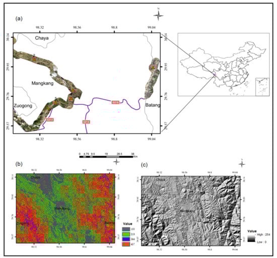
Figure 9.
(a) Study area with WorldView-3 data. (b) Average Slope Map of study area. (c) Hillshade Map of study area.
The input data were WorldView-3 satellite images, including panchromatic images with a 0.31 m spatial resolution and 8-band multispectral imagery with a resolution of 1.24 m. With an area of 396 km2, the study area primarily covered a 5 km-long strip centered on the G318 and G214 national highways, where there were intensive human activities. The images used received fusion, color correction, mosaics, and geometric correction.
The datasets were labeled into the following five classes: building, forest, water, road, and bare land. 518 samples (size 3201 × 3201) were labeled manually pixel-by-pixel, each of which corresponded to labeled data annotated at the pixel level (Figure 10). Invalid samples with poor qualities due to black edges, clouds, and shadows were manually deleted, resulting in 300 pairs of valid experimental data, 296 pairs of which were used for sampling and the remaining four for testing.
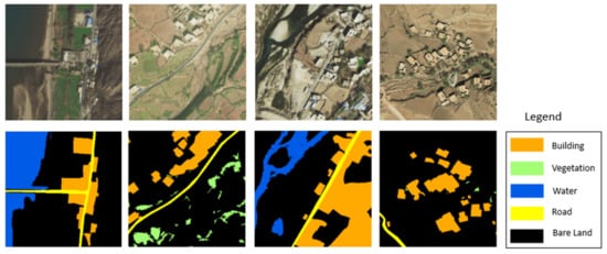
Figure 10.
Labeled data corresponding to Mangkam training dataset.
In this study, 296 image-label pairs (size 3200 × 3200) were superpixel-segmented to obtain the WorldView-3 image labeling dataset with images of size 512 × 512. The original dataset is composed of 6435 image-label pairs, and the spatial resolution is 1.24 m
As shown in Figure 11, over 90% of the samples were distributed in forest and bare land, while the total proportion of the remaining three classes was smaller than 3% in this sample set. The proportions of roads (0.36%) and buildings (0.51%) were low, suggesting that there was a significant imbalance in the proportions of different classes.
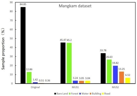
Figure 11.
Sample proportion (%) of different classes in original and multistage sampling of Mangkam (MUS1, MUS2).
Moreover, other training dataset is collected with GF-2 high-resolution remote sensing images (true color fusion images with 0.8 m resolution) of northeastern Beijing, China. These datasets were selected for the following reasons: (1) both datasets are very-high-spatial-resolution images, which can examine our classification method, and (2) they correspond to different scenarios. One is peri-urban and the other is a dense urban area.
In the GF-2 training dataset, we selected totally 89 samples (size 1600 × 1600) which is of imbalanced data. For each image, there exists a label map following six classes: building, forest, water, road, shadow, and bare land (Figure 12). We use 89 images of them for training, and the remaining four images for testing.
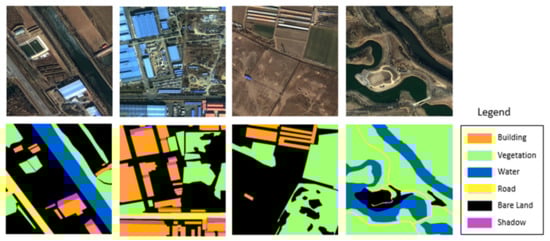
Figure 12.
Labeled data corresponding to Northeastern Beijing training dataset.
As shown in Figure 13, for different classes in the datasets illustrate the significantly imbalanced distribution of samples over the different object classes. In the datasets, over 90% of the samples are distributed between only three classes, while the remaining three classes are represented altogether by less than 10% of the samples, representing an imbalanced dataset.
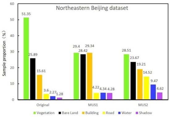
Figure 13.
Sample proportion (%) of different classes in original and multistage sampling of Northeastern Beijing (MUS1, MUS2).
3.2. Sampling the Datasets
Valuable training sample sets were obtained using multistage sampling. The sample proportions for Mangkam after valid sampling were shown in Figure 11. A total of 2000 images (size 512 × 512) that corresponded to 2000 labels were obtained after sampling. During the first stage, the proportions of sample in the minority classes, such as water, buildings and roads, in the total number of samples were increased. The sample proportions in the majority classes, such as bare land, were reduced. The sample proportions of MUS1 training set with were shown in Figure 11 (MUS1). The second stage was carried out to reach a rough balance between all the classes, thereby ensuring that the samples from every class could contribute to the training with as little bias as possible. Figure 11 (MUS2) showed that the constant of our MUS2 training after multistage sampling set is about equal to 6.8.
The sample proportions for northeastern Beijing after valid sampling were shown in Figure 11. A total of 1500 images (size 512 × 512) that corresponded to 1500 labels were obtained, and the sample proportions of MUS1 training set with were shown in Figure 13 (MUS1). The constant of MUS2 training is about equal to 4.76 (Figure 13 (MUS2)).
3.3. Training and Metrics
Anaconda was used for our approach based on the TensorFlow machine learning framework in Linux. The experimental platform configuration was as follows: Inter Xeon E5- 2650 3.5 GHz and four NVidia Tesla K80s. An Encoder-Decoder with ASPP was used with Xception20 as the core algorithm. The training was carried out using SGD for 100 epochs. A “step” policy for the learning rate adjustment (gamma = 0.1, step-size = 15,000) was used during each epoch. The closer it was to the error minimum, the smaller the step length was. After each convolutional layer, batch normalization was used for optimization, to accelerate convergence, and to reduce the number of epochs. Training efficiency was enhanced by about 10 times because it was unnecessary to train the neural network to adapt to the data distribution. The data were “trimmed” using the activation function to reduce the diffusion of gradients. The base learning rate was 0.01. The basic parameters for calculating the increments were m = 0.9 and dw = 0.0005. The maximum number of iterations in training stage of two datasets was 29,300 and 40,000 respectively. In the training procedure, we first randomly shuffled the samples, and subsequently fed them into the network in batches. Each batch contained eight images.
Test data were predicted using the trained model, and the classification result was obtained. Actual label data were used to evaluate their accuracy. In this study, the influences of different distributions of the sample proportions on four network models (basic FCN, FCN-8S, ASPP, and the proposed Encoder-Decoder with ASPP) were compared. The training sample set was derived from the multistage sampling result. Sample proportions were shown in Figure 11 and Figure 13 (Original, MUS1, and MUS2). In addition, the classification performance of different network models was evaluated.
To ensure consistency in the algorithm comparison, the same sets of training and test data were used for the four models. In addition, considered with the imbalanced dataset, it could be easier to obtain high accuracy without actually making useful predictions. Because of the accuracy as an evaluation, metrics will make sense only if the class labels of test data are uniformly distributed. So in this paper the performance of the various methods was evaluated based on the criteria as following: per-class precision, overall accuracy (OA), average recall, average -score and G-mean, which are considered to be easily interpretable and have better theoretical properties than other classification measures for class imbalanced problems [56]. Mutual usage of the G-mean measure and overall accuracy is considered in the evaluation of sampling schema in order to achieve the optimal performance for both majority and minority classes.
The precision was defined as the number of true positives (TP) divided by the sum of the number of true positives (TP) and false positives (FP):
The recall was defined as the number of true positives (TP) divided by the sum of the number of true positives (TP) and false negatives (FN):
The overall accuracy was defined as follows:
In addition, was defined as follows:
G-mean is considered as one of the most appropriate metrics where the performance of all classes is concerned and is adapted from true positive rate and true negative rate measures, which was defined as follows:
3.4. Experimental Result
The classification accuracies after training using four different models (basic FCN, FCN-8s, ASPP, and Encode-Decoder with ASPP) with training sets original class distribution (ORG), MUS1, and MUS2 as inputs were presented in Table 1 and Table 2. The result of training set with the original proportion indicated that all the network models performed poorly in the classification. Along with the training sets reaching balanced distributions from MUS1 to MUS2, classification accuracy and G-mean of the same network model also varied. The G-mean values, however, increased significantly as a result of changing the data distribution.

Table 1.
Comparison between approaches using Basic FCN, FCN-16s, FCN-8s, ASPP, Encoder-Decoder with ASPP, and our approach for classification on the Mangkam dataset.
Table 2.
Comparison between approaches using SVM, Basic FCN, FCN-16s, FCN-8s, ASPP, Encoder-Decoder with ASPP, and our approach for classification on the Northeastern Beijing dataset.
With MUS2 of Mangkam dataset, our sampling approach and Encode-Decoder with ASPP model obtained highest OA value of 0.88 and G-mean value of 0.84 among the 12 classification methods, which is a 0.07 and 0.27 relative improvement from the original dataset. There were significant changes in the classification accuracies for minority classes: the accuracies of road identification were enhanced by 0.53 and those of building identification were enhanced by 0.52.
The classification result for roads in Mangkam images was the lowest in every model. The reason was that roads still contained few pixels after data sampling, for which information loss was more likely to occur during pooling. In addition, buildings and roads highly resembled bare land and required a large number of samples in the sets. Thus, the classification result for the minority classes might not be ideal due to class confusion. We showed a visual comparison of the classified images in Figure 14.
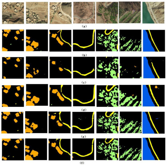
Figure 14.
Classification results for Mangkam images (Experiment A): (a) Original images; (b) GT labels corresponding to the images in (a); (c–e) results of MUS2 + BasicFCN, MUS2 + FCN-8s, and MUS2 + ASPP classification corresponding to the images in (a), respectively; and (f) our classification results corresponding to the images in (a).
With MUS2 of northeastern Beijing dataset, our sampling approach and Encoder-Decoder with ASPP model also achieved highest OA value of 0.89 and G-mean value of 0.88, and above all, for the minority classes, the above statistics show our approach obtains the best performance compared with the others. Figure 15 illustrates the result of our proposed approach.
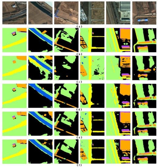
Figure 15.
Classification results for Northeastern Beijing images (Experiment B): (a) Original images; (b) GT labels corresponding to the images in (a); (c–e) results of MUS2 + BasicFCN, MUS2 + FCN-8s, and MUS2 + ASPP classification corresponding to the images in (a), respectively; and (f) our classification results corresponding to the images in (a).
4. Discussion
4.1. The Importance of Data Segmentation
To obtain sufficient quality training data, data segmentation is the pre-processing that pre-segments the training set into patches via the SILC algorithm. Different from random cropping that lacks relevance to the ground objects, superpixel segmentation could be used to find regions that might contain low variability in the image.
Generating complete object images and corresponding label data help to use samples efficiently in the training stage. Consequently, trained deep learning models also can achieve a better classification performance. As shown in Table 3, for overall accuracy, the data segmentation brings 0.16 and 0.14 improvement on the Mangkam and the Northeastern Beijing datasets respectively. Meanwhile, G-Mean, recall and F1-score have also been improved. Experiments based on two datasets show that assembling data segmentation with Encoder-Decoder with ASPP model can obtain improvement on classification accuracy.
Table 3.
The comparison result of assembling random cropping or superpixel segmentation with Encoder-Decoder with ASPP model.
4.2. Comparison with Other Methods to Address Imbalance
Regarding performance of different methods for addressing imbalance, the influence of different sampling schema (random over-sampling, random under-sampling, SMOTE over-sampling, identical sampling, and multistage sampling) and weighting on the final classification result were compared based on the Encoder-Decoder with ASPP. We evaluated the classification performance (especially the classification accuracy for minority classes) on Mangkam dataset after adapting these six methods.
In two weighting experiments, the values of weights in the loss function were denoted LOSS1 (bare land: 1; building: 2; road: 2; water: 1; forest: 1) and LOSS2 (bare land: 1; building: 4; road: 4; water: 1; forest: 1). For minority classes of dataset, the SMOTE algorithm was applied with an over-sampling index of up to 235 depending on distribution of the sample proportions, to generate a certain number of synthetic samples along the linking paths to the neighbors. Table 4 shows the SMOTE over-sampling index for per-class. Different from taking identical number of samples from classes using identical sampling, the training sample sets of the multistage sampling were shown in Figure 11 (MUS1 and MUS2). The influence of five sampling schema and cost weighting on the final classification performance of the Encoder-Decoder with ASPP network were shown in Table 4. In this section, the sensitivities of the network models to the weight of the loss function and training sample distribution were quantitatively presented.
Table 4.
Comparison between LOSS1, LOSS2, random over-sampling, random under-sampling, SMOTE over-sampling, identical sampling, MUS1, and MUS2.
As seen in Table 4, the recall for road and building achieved higher value results than that of the original results combined with these methods, while MUS2 outperforms the rest in all circumstances. Although the differences between the OA values were trivial under all methods, the G-mean varied significantly due to different accuracies for minority classes of imbalanced dataset. Furthermore, the MUS2 gained the highest overall classification accuracy (0.88), G-Mean (0.84), and recall for buildings (0.82) and roads (0.73).
Based on the results, high classification accuracies for buildings and roads in the study area could not be guaranteed by directly setting the weight of each class in the deep neural network. This result supported the hypothesis that the classification accuracy of each class could be enhanced by combining the sampling method and classifier.
Different sampling methods can result in different accuracy levels. A combination of SMOTE over-sampling improved both the G-mean and recall for minority classes compared to the corresponding values in the original dataset. While the number of synthetic samples generated is much larger than the number of real-world ones, samples of invalid information may not result in the desired accuracy, particularly for skewed datasets. Even though improving recall for minority classes, using identical sampling resulted in considerably low overall accuracy. This could be attributed to the reasons of underrepresentation of the training samples from the minority classes during identical sampling, or the information deficiency for majority classes when minority classes are over represented, since low overall accuracy mean samples from majority classes have been wrongly labelled as members of these minority classes. Regarding performance of different methods for addressing imbalance, multistage sampling may be the excellent method in performance.
4.3. Comparison of Classifier Algorithm for Classification
This paper presents a classification approach for high-resolution images using the Encoder-Decoder with ASPP model. We evaluated our approach in the comparison to object-oriented SVM classification. Object-oriented approach was conducted using the multi-resolution segmentation and SVM classification. Firstly, multi-resolution segmentation was implemented by the tuning scale, shape, and compactness parameters (60, 0.2, and 0.5) to obtain high-quality image objects. Then, we selected the most representative features for the following SVM classification, including mean value and brightness for each band; density and length-width ratio of the image object; GLCM-mean value; GLDV-mean. The kernel function we used in SVM is the radial basis function (RBF), and the optimal penalty factor C and kernel function parameter γ used for SVM classifier were 100 and 0.005, respectively. According to the of the sample proportions of classes in the original Mangkam dataset, we select the same proportion distribution of the image objects from each image as samples.
As shown in Table 5, Object-oriented with SVM classification has shown good classification performance in minority classes (0.76 and 0.69 respectively recall for building and road), the same as in terms of the G-mean measure. Given the low overall accuracy of object-oriented classification having, our approach seemed to perform better than this classifier applied to the original training dataset.
Table 5.
Comparison with object-oriented classification approach on the test Mangkam data.
While samples of minority classes near the class boundary were chosen as support vectors, SVM as a classifier is insensitive to data imbalance, and can achieve results of high accuracy for minority classes. Some selection of expressive features also contributes to identification of boundary in classification stage. The prediction result was shown in Figure 16c. Instead of inputting features of samples to the classifier, which depends on experience and extensive attempts, our deep-learning-based model can utilize all of the image information to implement feature extraction and classification.
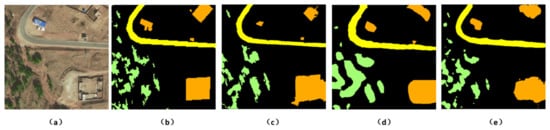
Figure 16.
Detail comparison of object-oriented classification on original Mangkam data, basic FCN and our approach both training on the Mangkam MUS2 dataset: (a) original images; (b) GT labels corresponding to the images in (a); (c) classification result from Object-oriented with SVM; (f) classification result from Basic FCN; and (e) classification result from our approach.
Comparing our four typical deep-learning-based approaches, the classification performance is obviously improved. In the following sections, we will discuss the reasons. Figure 16d shows that the prediction result of basic FCN for forest tends to output blob-like objects because resolution is significantly reduced due to the pooling of basic FCN. Basic FCN was unable to achieve multiscale segmentation. Comparatively, the Encoder-Decoder with ASPP network performed better in retaining forest details than Basic FCN.
With the MUS2 training set, there were significant differences between the classification results for road and bare land (Figure 17c–e). As shown in Figure 17c, the boundaries of the roads and bare land were discontinuous, and the bare land was clearly divided into two parts. Such an obviously incorrect result can be attributed to the fact that the lost resolution is compensated by deconvolution operation in FCN-8S model. However, it was difficult for deconvolution to effectively recover the resolution through learning. The classification result in Figure 17d was markedly enhanced because the shapes of the roads and bare land were basically retained. However, there were still visible plaques and losses along the boundaries, because parallel sampling using atrous convolution with different sampling rates was applied in the ASPP, and the boundary details could not be fully recovered by obtaining the expected dimensions using bilinear up sampling by a factor of 16. As shown in Figure 17e, the results of the Encoder-Decoder with ASPP network were close to the real labels; the classification accuracies with this model were significantly enhanced. This model played a role in restoring object boundaries by capturing multilayer contextual information and distance information in the Encoder stage and recovering the details and spatial dimensions of the targets using the information obtained during the Encoder stage in the Decoder stage. Thus, the classes predicted were further refined.
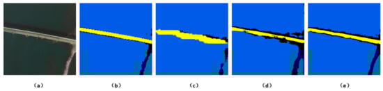
Figure 17.
Detail comparison of edge information generated by FCN 8s, ASPP, and our approach training on the Mangkam MUS2 dataset: (a) original images; (b) GT labels corresponding to the images in (a); (c) classification result from FCN 8s; (d) classification result from ASPP; and (e) classification result from our approach.
4.4. Applications and Limitations of Our Approach
Owing to the wide differences between the areas of various ground objects, their uneven distribution, the small sizes of target features, and other factors in the study area, as well as the number of pixels they occupied in the high-resolution remote sensing images differed significantly. The imbalanced data also suggested that there was a great difference between the proportions of training samples included in the supervised classification.
Deep neural network methods were able to organize multilayer neurons to learn more expressive features from large volumes of training data. Accurate automatic ground object information with target details could be extracted by applying a deep-learning-based Encoder-Decoder with ASPP model for pixel-level classification of high-resolution remote sensing images.
As an important and effective supervised image classification framework, this model required a large number of annotated samples for training. Both the quantity and quality of samples were directly associated with the algorithm application and final accuracy of the result. The training sample imbalance would undermine the classification performance of deep neural networks [39]. Algorithm- and dataset-oriented methods are two major types suitable for use on imbalanced data: It is critical to select an appropriate scheme to improve the final classification performance of the study area. The experiment results indicated that a high overall classification accuracy could be obtained by improving the classification network model, but this method still performed unsatisfactorily in identifying minority classes. Compared with the weighting loss, the proposed method of multistage sampling, particularly in the MUS2 stage, was able to significantly improve the classification performance of minority classes.
High-quality real ground object labeling depended highly on the experience of classification personnel. For better applicability, semi-supervised learning methods could be used to investigate other remote sensing data sources in future studies.
Deep -learning-based application scenarios and technical roadmaps for high-resolution remote sensing image classification were proposed in this study. Automatic prediction could be realized by means of image pre-processing, sample labeling, multistage sampling, and model training using the samples, which not only significantly reduced human costs and time, but also ensured the interpretation accuracy of the surface environment. This framework had the potential to adapt to a wider range of engineering and multi-source remote sensing satellite data.
5. Conclusions
In this study, a classification task for imbalanced data of high-resolution remote sensing images was researched using the deep -learning-based model of Encoder-Decoder with ASPP. According to the results, the following conclusions were obtained:
- The network used in the experiment was an ASPP-based model combining Encoder and Decoder stages. Atrous convolution and ASPP were used to obtain high-resolution class prediction in the Encoder stage, and the boundary details of the targets were recovered in the Decoder stage. This algorithm could adapt to the large amount of complex ground object details for the processing of high-resolution remote sensing images. Compared with other network models (e.g., basic FCN, FCN-8S, and ASPP), the proposed model fully took advantage of the features of high-resolution remote sensing images, and the overall highest classification accuracy is obviously improved.
- We employed two datasets of labeled high-resolution remote sensing images to train deep neural networks. Both two study area possessed imbalanced class distribution. A multistage sampling technique was used to obtain MUS2, where the proportions of the ground objects were more balanced. The G-Mean value obtained using the model trained by MUS2 reached as high as 0.84 and 0.88 respectively, and those for minority were also significantly enhanced.
Author Contributions
Conceptualization, W.X.; Data curation, Z.Y. and J.D.; Formal analysis, W.X.; Methodology, W.X.; Software, S.L.; Supervision, J.L. and F.C.; Writing—original draft, W.X.; Writing—review & editing, C.M.
Funding
National Natural Science Funds for Key Projects of China: 61731022; Hainan Provincial Natural Science Foundation of China: 618QN303; National Key R&D Program of China (Grant No. 2018YFE010010001-3, No. 2018YFC0809400); the Science and Technology project of State Grid (Grant No. 5442GY180025).
Acknowledgments
The authors thank the editors and the reviewers for their valuable comments to improve our manuscript.
Conflicts of Interest
The authors declare no conflicts of interest.
References
- Jat, M.K.; Garg, P.K.; Khare, D. Monitoring and modelling of urban sprawl using remote sensing and gis techniques. Int. J. Appl. Earth Obs. Geoinf. 2008, 10, 26–43. [Google Scholar] [CrossRef]
- Melesse, A.; Weng, Q.; Thenkabail, P.; Senay, G. Remote sensing sensors and applications in environmental resources mapping and modelling. Sensors 2007, 7, 3209–3241. [Google Scholar] [CrossRef] [PubMed]
- Watts, A.C.; Ambrosia, V.G.; Hinkley, E.A. Unmanned aircraft systems in remote sensing and scientific research: Classification and considerations of use. Remote Sens. 2012, 4, 1671–1692. [Google Scholar] [CrossRef]
- Weng, Q.; Lu, D. Landscape as a continuum: An examination of the urban landscape structures and dynamics of indianapolis city, 1991–2000, by using satellite images. Int. J. Remote Sens. 2009, 30, 2547–2577. [Google Scholar] [CrossRef]
- MacQueen, J. Some methods for classification and analysis of multivariate observations. In Proceedings of the Fifth Berkeley Symposium on Mathematical Statistics and Probability, Oakland, CA, USA, 21 June 1967; pp. 281–297. [Google Scholar]
- Zhong, Y.; Zhang, L.; Huang, B.; Li, P. An unsupervised artificial immune classifier for multi/hyperspectral remote sensing imagery. IEEE Trans. Geosci. Remote Sens. 2006, 44, 420–431. [Google Scholar] [CrossRef]
- Friedl, M.A.; McIver, D.K.; Hodges, J.C.; Zhang, X.Y.; Muchoney, D.; Strahler, A.H.; Woodcock, C.E.; Gopal, S.; Schneider, A.; Cooper, A. Global land cover mapping from modis: Algorithms and early results. Remote Sens. Environ. 2002, 83, 287–302. [Google Scholar] [CrossRef]
- Miller, D.M.; Kaminsky, E.J.; Rana, S. Neural network classification of remote-sensing data. Comput. Geosci. 1995, 21, 377–386. [Google Scholar] [CrossRef]
- Mountrakis, G.; Im, J.; Ogole, C. Support vector machines in remote sensing: A review. ISPRS J. Photogramm. Remote Sens. 2011, 66, 247–259. [Google Scholar] [CrossRef]
- Rodriguez-Galiano, V.F.; Ghimire, B.; Rogan, J.; Chica-Olmo, M.; Rigol-Sanchez, J.P. An assessment of the effectiveness of a random forest classifier for land-cover classification. ISPRS J. Photogramm. Remote Sens. 2012, 67, 93–104. [Google Scholar] [CrossRef]
- Lu, D.; Weng, Q. Use of impervious surface in urban land-use classification. Remote Sens. Environ. 2006, 102, 146–160. [Google Scholar] [CrossRef]
- Chen, Y.; Su, W.; Li, J.; Sun, Z. Hierarchical object oriented classification using very high resolution imagery and lidar data over urban areas. Adv. Space Res. 2009, 43, 1101–1110. [Google Scholar] [CrossRef]
- Myint, S.W.; Gober, P.; Brazel, A.; Grossman-Clarke, S.; Weng, Q. Per-pixel vs. Object-based classification of urban land cover extraction using high spatial resolution imagery. Remote Sens. Environ. 2011, 115, 1145–1161. [Google Scholar] [CrossRef]
- Fu, G.; Liu, C.; Zhou, R.; Sun, T.; Zhang, Q. Classification for high resolution remote sensing imagery using a fully convolutional network. Remote Sens. 2017, 9, 498. [Google Scholar] [CrossRef]
- Raschka, S. When does Deep Learning Work Better Than Svms or Random Forests? Available online: https://www.kdnuggets.com/2016/04/deep-learning-vs-svm-random-forest.html (accessed on 22 April 2016).
- Jia, F.; Lei, Y.; Lin, J.; Zhou, X.; Lu, N. Deep neural networks: A promising tool for fault characteristic mining and intelligent diagnosis of rotating machinery with massive data. Mech. Syst. Signal Process. 2016, 72, 303–315. [Google Scholar] [CrossRef]
- Cambria, E. Affective computing and sentiment analysis. IEEE Intell. Syst. 2016, 31, 102–107. [Google Scholar] [CrossRef]
- Hu, F.; Xia, G.-S.; Hu, J.; Zhang, L. Transferring deep convolutional neural networks for the scene classification of high-resolution remote sensing imagery. Remote Sens. 2015, 7, 14680–14707. [Google Scholar] [CrossRef]
- LeCun, Y.; Bottou, L.; Bengio, Y.; Haffner, P. Gradient-based learning applied to document recognition. Proc. IEEE 1998, 86, 2278–2324. [Google Scholar] [CrossRef]
- Ren, S.; He, K.; Girshick, R.; Sun, J. Faster r-cnn: Towards real-time object detection with region proposal networks. In Advances in Neural Information Processing Systems (NIPS); Curran Associates, Inc.: Montreal, QC, Canada, 2015; pp. 91–99. [Google Scholar]
- Krizhevsky, A.; Sutskever, I.; Hinton, G.E. Imagenet classification with deep convolutional neural networks. In Advances in Neural Information Processing Systems (NIPS); Curran Associates, Inc.: Lake Tahoe, NV, USA, 2012; pp. 1097–1105. [Google Scholar]
- Long, J.; Shelhamer, E.; Darrell, T. Fully convolutional networks for semantic segmentation. In Proceedings of the IEEE Conference on Computer Vision and Pattern Recognition (CVPR); IEEE: Boston, MA, USA, 2015. [Google Scholar]
- Yu, F.; Koltun, V. Multi-scale context aggregation by dilated convolutions. arXiv 2015, arXiv:1511.07122. [Google Scholar]
- Zheng, S.; Jayasumana, S.; Romera-Paredes, B.; Vineet, V.; Su, Z.; Du, D.; Huang, C.; Torr, P.H. Conditional random fields as recurrent neural networks. In Proceedings of the IEEE International Conference on Computer Vision (CVPR); IEEE: Santiago, Chile, 2015. [Google Scholar]
- Chen, L.-C.; Papandreou, G.; Kokkinos, I.; Murphy, K.; Yuille, A.L. Semantic image segmentation with deep convolutional nets and fully connected crfs. arXiv 2014, arXiv:1412.7062. [Google Scholar]
- Chen, L.-C.; Papandreou, G.; Kokkinos, I.; Murphy, K.; Yuille, A.L. Deeplab: Semantic image segmentation with deep convolutional nets, atrous convolution, and fully connected crfs. IEEE Trans. Pattern Anal. Mach. Intell. 2017, 40, 834–848. [Google Scholar] [CrossRef]
- Chen, L.-C.; Papandreou, G.; Schroff, F.; Adam, H. Rethinking atrous convolution for semantic image segmentation. arXiv 2017, arXiv:1706.05587. [Google Scholar]
- Badrinarayanan, V.; Kendall, A.; Cipolla, R. Segnet: A deep convolutional encoder-decoder architecture for image segmentation. IEEE Trans. Pattern Anal. Mach. Intell. 2017, 39, 2481–2495. [Google Scholar] [CrossRef] [PubMed]
- Chen, L.-C.; Zhu, Y.; Papandreou, G.; Schroff, F.; Adam, H. Encoder-decoder with atrous separable convolution for semantic image segmentation. In Proceedings of the European Conference on Computer Vision (ECCV 2018); Springer: Salt Lake City, UT, USA, 2018; pp. 801–818. [Google Scholar]
- Li, Y.; Zhang, H.; Xue, X.; Jiang, Y.; Shen, Q. Deep learning for remote sensing image classification: A survey. Wiley Interdiscip. Rev. Data Min. Knowl. Discov. 2018, 8, e1264. [Google Scholar] [CrossRef]
- Volpi, M.; Tuia, D. Dense semantic labeling of subdecimeter resolution images with convolutional neural networks. IEEE Trans. Geosci. Remote Sens. 2017, 55, 881–893. [Google Scholar] [CrossRef]
- Längkvist, M.; Kiselev, A.; Alirezaie, M.; Loutfi, A. Classification and segmentation of satellite orthoimagery using convolutional neural networks. Remote Sens. 2016, 8, 329. [Google Scholar] [CrossRef]
- Marmanis, D.; Datcu, M.; Esch, T.; Stilla, U. Deep learning earth observation classification using imagenet pretrained networks. IEEE Geosci. Remote Sens. Lett. 2016, 13, 105–109. [Google Scholar] [CrossRef]
- Yang, Y.; Newsam, S. Bag-of-visual-words and spatial extensions for land-use classification. In Proceedings of the 18th SIGSPATIAL International Conference on Advances in Geographic Information Systems; ACM: San Jose, CA, USA, 2010; pp. 270–279. [Google Scholar]
- Maggiori, E.; Tarabalka, Y.; Charpiat, G.; Alliez, P. Convolutional neural networks for large-scale remote-sensing image classification. IEEE Trans. Geosci. Remote Sens. 2017, 55, 645–657. [Google Scholar] [CrossRef]
- Kampffmeyer, M.; Salberg, A.-B.; Jenssen, R. Semantic segmentation of small objects and modeling of uncertainty in urban remote sensing images using deep convolutional neural networks. In Proceedings of the IEEE Conference on Computer Vision and Pattern Recognition Workshops (CVPRW); IEEE: Las Vegas, NV, USA, 2016. [Google Scholar]
- Kussul, N.; Lavreniuk, M.; Skakun, S.; Shelestov, A. Deep learning classification of land cover and crop types using remote sensing data. IEEE Geosci. Remote Sens. Lett. 2017, 14, 778–782. [Google Scholar] [CrossRef]
- Wang, Y.; Liang, B.; Ding, M.; Li, J. Dense semantic labeling with atrous spatial pyramid pooling and decoder for high-resolution remote sensing imagery. Remote Sens. 2019, 11, 20. [Google Scholar] [CrossRef]
- Buda, M.; Maki, A.; Mazurowski, M.A. A systematic study of the class imbalance problem in convolutional neural networks. Neural Netw. 2018, 106, 249–259. [Google Scholar] [CrossRef]
- Ganganwar, V. An overview of classification algorithms for imbalanced datasets. Int. J. Emerg. Technol. Adv. Eng. 2012, 2, 42–47. [Google Scholar]
- López, V.; Fernández, A.; García, S.; Palade, V.; Herrera, F. An insight into classification with imbalanced data: Empirical results and current trends on using data intrinsic characteristics. Inf. Sci. 2013, 250, 113–141. [Google Scholar] [CrossRef]
- Ayhan, B.; Kwan, C. A comparative study of two approaches for uav emergency landing site surface type estimation. In Proceedings of the IECON 2018-44th Annual Conference of the IEEE Industrial Electronics Society, Washington, DC, USA, 21–23 October 2018; pp. 5589–5593. [Google Scholar]
- Sun, Y.; Kamel, M.S.; Wong, A.K.; Wang, Y. Cost-sensitive boosting for classification of imbalanced data. Pattern Recognit. 2007, 40, 3358–3378. [Google Scholar] [CrossRef]
- Lu, Y.; Cheung, Y.-M.; Tang, Y.Y. Hybrid sampling with bagging for class imbalance learning. In Pacific-Asia Conference on Knowledge Discovery and Data Mining; Springer: Berlin, Germany, 2016; pp. 14–26. [Google Scholar]
- Han, H.; Wang, W.-Y.; Mao, B.-H. Borderline-smote: A new over-sampling method in imbalanced data sets learning. In International Conference on Intelligent Computing; Springer: Berlin, Germany, 2005; pp. 878–887. [Google Scholar]
- Liu, X.-Y.; Wu, J.; Zhou, Z.-H. Exploratory undersampling for class-imbalance learning. IEEE Trans. Syst. Man Cybern. Part B Cybern. 2009, 39, 539–550. [Google Scholar]
- Galar, M.; Fernandez, A.; Barrenechea, E.; Bustince, H.; Herrera, F. A review on ensembles for the class imbalance problem: Bagging-boosting-and hybrid-based approaches. IEEE Trans. Syst. Man Cybern. Part C Appl. Rev. 2012, 42, 463–484. [Google Scholar] [CrossRef]
- He, H.; Bai, Y.; Garcia, E.; Li, S.A. Adaptive synthetic sampling approach for imbalanced learning. In IEEE International Joint Conference on Neural Networks, 2008 (IEEE World Congress on Computational Intelligence); IEEE: Piscataway, NJ, USA, 2008. [Google Scholar]
- Tahir, M.A.; Kittler, J.; Yan, F. Inverse random under sampling for class imbalance problem and its application to multi-label classification. Pattern Recognit. 2012, 45, 3738–3750. [Google Scholar] [CrossRef]
- Chawla, N.V. Data mining for imbalanced datasets: An overview. In Data Mining and Knowledge Discovery Handbook; Springer: Berlin, Germany, 2009; pp. 875–886. [Google Scholar]
- Japkowicz, N.; Stephen, S. The class imbalance problem: A systematic study. Intell. Data Anal. 2002, 6, 429–449. [Google Scholar] [CrossRef]
- Akbani, R.; Kwek, S.; Japkowicz, N. Applying support vector machines to imbalanced datasets. In European Conference on Machine Learning; Springer: Berlin, Germany, 2004; pp. 39–50. [Google Scholar]
- Tang, Y.; Zhang, Y.-Q.; Chawla, N.V.; Krasser, S. Svms modeling for highly imbalanced classification. IEEE Trans. Syst. Man Cybern. Part B Cybern. 2009, 39, 281–288. [Google Scholar] [CrossRef]
- Azadbakht, M.; Fraser, C.S.; Khoshelham, K. Synergy of sampling techniques and ensemble classifiers for classification of urban environments using full-waveform lidar data. Int. J. Appl. Earth Obs. Geoinf. 2018, 73, 277–291. [Google Scholar] [CrossRef]
- Chawla, N.V.; Bowyer, K.W.; Hall, L.O.; Kegelmeyer, W.P. Smote: Synthetic minority over-sampling technique. J. Artif. Intell. Res. 2002, 16, 321–357. [Google Scholar] [CrossRef]
- Brzezinski, D.; Stefanowski, J.; Susmaga, R.; Szczȩch, I. Visual-based analysis of classification measures and their properties for class imbalanced problems. Inf. Sci. 2018, 462, 242–261. [Google Scholar] [CrossRef]
© 2019 by the authors. Licensee MDPI, Basel, Switzerland. This article is an open access article distributed under the terms and conditions of the Creative Commons Attribution (CC BY) license (http://creativecommons.org/licenses/by/4.0/).