Abstract
As a key parameter that represents the structural characteristics and biophysical changes of crop canopy, the leaf area index (LAI) plays a significant role in monitoring crop growth and mapping yield. A considerable amount of farmland is dispersed with strong spatial heterogeneity. The existing time series satellite LAI products fail to capture spatial distributions and growth changes of crops due to coarse spatial resolutions and spatio-temporal discontinuities. Therefore, it becomes crucial for fine resolution LAI mapping in time series over crop areas. A two-stage data assimilation scheme was developed for dense time series LAI mapping in this study. A LAI dynamic model was first constructed using multi-year MODIS LAI data. This model coupled with the PROSAIL radiative transfer model, and MOD09A1 reflectance data were used to retrieve temporal LAI profiles at the 500 m resolution with the assistance of the very fast simulated annealing (VFSA) algorithm. Then, the LAI dynamics at the 500 m scale were incorporated as prior information into the Landsat 8 OLI reflectance data for time series LAI mapping at the 30 m resolution. Finally, the spatio-temporal continuities and retrieval accuracies of assimilated LAI values were assessed at the 500 m and 30 m resolutions respectively, using the MODIS LAI product, fine resolution LAI reference map and field measurements. The results indicated that the assimilated the LAI estimations at the 500 m scale effectively eliminated the spatio-temporal discontinuities of the MODIS LAI product and displayed reasonable temporal profiles and spatial integrity of LAI. Moreover, the 30 m resolution LAI retrievals showed more abundant spatial details and reasonable temporal profiles than the counterparts at the 500 m scale. The determination coefficient R2 between the estimated and field LAI values was 0.76 with a root mean square error (RMSE) value of 0.71 at the 30 m scale. The developed method not only improves the spatio-temporal continuities of the LAI at the 500 m scale, but also obtains 30 m resolution LAI maps with fine spatial and temporal consistencies, which can be expected to meet the needs of analysis on crop dynamic changes and yield mapping in fragmented and highly heterogeneous areas.
1. Introduction
Monitoring local crop production is very critical for national food security and sustainable development of agriculture. Therefore, it is remarkably significant to carry out the growth-monitoring and yield estimation of crops. The leaf area index (LAI) derived from remotely sensed data is an important parameter monitoring crop growth and estimating yield at regional or global scales [1,2,3]. The LAI directly denotes photosynthesis, transpiration efficiency and the energy balance of plants [4,5]. Generally, it is defined as the sum of one-side green leaf areas per unit surface area [6].
At present, various kinds of remotely sensed LAI products have been released free of charge, such as MODIS LAI [7], GLASS LAI [8] and GEOV1 LAI [9]. However, most of them are retrieved from instantaneous satellite observations, without considering the phenological variations of different crops [10,11]. Subsequently, these products sometimes hold poor data quality and abnormal fluctuations in the time series due to the effects of cloud contaminations, satellite sensors, retrieval algorithms, etc [12]. The existing multi-temporal LAI products behave poorly and show significant differences in seasonal characterizations over mountainous areas [5]. Moreover, from the perspective of spatial dimensions, the crop areas are usually composed of multiple land cover types, which easily leads to strong spatial heterogeneity and fragmentation of farmlands. The current coarse spatial resolution (i.e., ≥500 m) LAI products fail to reasonably describe the distribution characteristics of farmlands in fragmented landscapes [5]. The product accuracies are hard to satisfy the needs of dynamic monitoring on crops. Therefore, it is necessary to spatially and temporally map continuous LAI from remotely sensed data in crop regions.
Fine resolution (e.g., 30 m) LAI mapping in the time series is expected to provide data support for crop growth monitoring and accurate yield estimations in fragile areas. In addition, most crop growth models strongly need fine spatial and temporal resolution LAI values as inputs for precision agriculture management and yield predictions. The image fusion techniques are beneficial to enhance the temporal and spatial resolutions of satellite-derived LAI with the help of temporal, spectral and spatial information from multi-resolution observations [13,14,15,16]. They generate single synthetic fine-resolution imagery at the prediction date when one or more observed pairs of coarse- and fine-resolution images for training and a coarse-resolution image at the prediction date are given as input data. However, the quality of a synthetic scene seems to degrade when the prediction date is far apart in time from the counterpart of observed pairs because of the weak fusion assumption in this case [15]. Furthermore, two or more fine-resolution images are required as input data so as to improve the performance of data fusion methods. Unfortunately, it is sometimes difficult to obtain two or more image pairs for training during the vegetation growing season owing to cloud coverage, the revisit period or other reasons [17]. Additionally, most data fusion techniques are not capable of describing abrupt changes of land cover types over heterogeneous surfaces [18]. These foregoing problems evidently constrain the applications of image fusion methods in the dense time series (rather than single) and fine resolution LAI mapping during crop growth season.
In recent years, land surface data assimilation methods [19] are considered as an attractive alternative to estimate spatially and temporally continuous LAI through the integration of remotely sensed observations and a crop growth model [20,21]. The data assimilation algorithms can introduce a crop growth model into satellite-based LAI retrievals, which fully utilizes the spatial advantages of satellite observations and the temporal characteristics of a crop model [19]. This practice is potential to improve the spatio-temporal continuities and retrieval accuracies of LAI mapping [22,23]. More importantly, data assimilation techniques are expected to generate fine spatio-temporal resolution LAI maps by fusing multiresolution (e.g., 1 km, 500 m, and 30 m), multitemporal and multisensor (e.g., MODIS and Landsat) satellite observations. [24,25] estimated the temporal high-resolution LAI by combining 1 km MODIS LAI products and ASTER/HJ CCD reflectance data through a dynamic Bayesian network. The coarse resolution LAI products were used to build an empirical crop growth model so as to depict the LAI variations in the time series. It is noted that the predictive performance of an empirical model built from satellite LAI products was sometimes limited by the quality of original LAI products themselves [22,23]. It is expected that an empirical crop growth model is constructed from the spatially and temporally continuous LAI assimilation results rather than the current LAI products, which subsequently may improve the retrieval accuracy of LAI at fine resolution.
In this context, this work aims to (1) eliminate the spatio-temporal discontinuities of existing LAI products (e.g., MODIS LAI) and map spatially and temporally continuous LAI at the 500 m resolution using a data assimilation technique, and (2) further improve fine spatial (i.e., 30 m) and temporal resolution LAI mapping in fragmented areas by downscaling the 500 m resolution LAI estimations.
2. Methodology
A two-stage data assimilation scheme was designed to map LAI dynamics at the 500 m and 30 m resolutions. At the 500 m scale, an empirical LAI dynamic model was first constructed using multi-year MODIS LAI products to describe the temporal variations of LAI. Then, the LAI dynamic model was coupled with the PROSAIL radiative transfer model to simulate crop canopy reflectance. Meanwhile, the high-quality reflectance data from the MOD09A1 product acquired during the crop growing season served as time series observations. The very fast simulated annealing (VFSA) algorithm was used to adjust the temporal LAI values so as to minimize the differences between the simulated and observed reflectance data. Thus, the time series LAI maps were derived at the 500 m resolution (Figure 1).
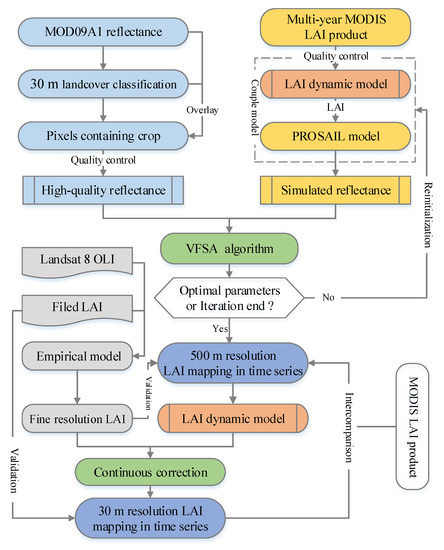
Figure 1.
Flowchart of spatially and temporally continuous crop leaf area index (LAI) mapping in crop areas.
At the 30 m spatial resolution, a new LAI dynamic model was first built from the 500 m scale LAI assimilations. Subsequently, the temporal LAI values were estimated using the continuous correction assimilation method through the combination of this dynamic model and LAI retrievals from Landsat 8 OLI data. Finally, the assimilated LAI results at the 500 m and 30 m scales were validated directly or indirectly from the aspects of spatial patterns, temporal variations and quantitative accuracy evaluations (Figure 1).
The introductions of an empirical LAI dynamic model, the PROSAIL model and the data assimilation methods are described in detail in Section 2.3 and Section 2.4, respectively.
2.1. Study Area
The study area (105°09″–105°50″E, 31°11″–31°24″N) is located in Yanting County, Mianyang City, Sichuan Province, China (Figure 2). The hills and low-mountains are the dominating landform types. The elevation gradually increases from south to north. The climate is a subtropical monsoon, with distinct seasons as well as concentrated precipitation. The study area is cross-distributed with paddy fields, dry lands and forests. Its summer crops are mainly rice and maize, the growing season of which is from April to October.
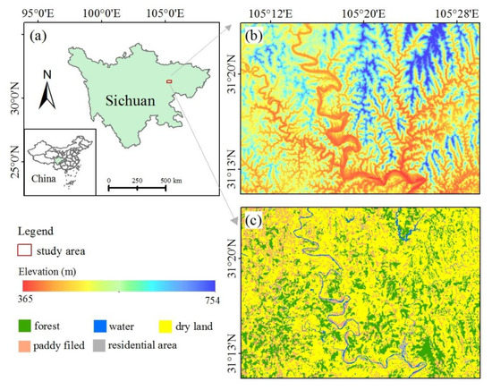
Figure 2.
Study area with the geographical location (a) elevation (b) and land cover types (c).
2.2. Data Sets
The data sets mainly include the MODIS LAI product MOD15A2H, bidirectional surface reflectance product MOD09A1, Landsat 8 surface reflectance data, field LAI measurements and the land cover map.
2.2.1. Field LAI Measurements
During 7–15 August, 2013, 57 square quadrats were designed in rice and maize cultivated areas, each of which is 30 m × 30 m in size. In each sampling quadrat, the field LAI measurements were collected at six subplots of 1 m × 1 m using the LAI-2200 plant canopy analyzer. One above-canopy incident radiation was firstly observed, and then eight below-canopy recordings were measured evenly for the LAI calculation in each subplot. The LAI value was taken as the average of six LAI samples in each quadrat. The selections of quadrats mainly followed the principles of spatial representativeness and sampling accessibility. Considering the effective LAI obtained from LAI-2200 was prone to be underestimated when the crop leaves were not randomly distributed, the effective values were transformed into real the LAIs using the clumping index [26]. The field LAI measurements were mainly used to carry out accuracy evaluation of the LAI assimilation at the 30 m resolution.
2.2.2. MODIS Products
(1) MODIS LAI Product
The collection 6 MODIS LAI product MOD15A2H with an 8-day temporal interval and a 500 m sinusoidal grid from 2000 to 2013 was downloaded from https://search.earthdata.nasa.gov/. The retrieval methods of MOD15A2H product include the main algorithm and the backup one. The former uses a three-dimensional radiation transfer model to construct a lookup table for LAI retrieval. When the main algorithm fails, the back-up algorithm would be used to retrieve LAI based on the empirical statistical relationships between the LAI and normalized difference vegetation index (NDVI) across different vegetation types [27]. Note that no significant changes existed in the structural attributes of the study area during 2000 to 2013 through the field campaigns and a questionnaire-based survey. Therefore, the mean MODIS LAI values derived from the main algorithm during 2000 to 2012 were applied to construct an empirical LAI dynamic model, which provided prior knowledge for retrieving the time series LAI at the 500 m resolution. The MODIS LAI product in 2013 was used as indirect references to evaluate the assimilated LAI results.
(2) MODIS reflectance product
The bidirectional reflectance product MOD09A1 has a spatial resolution of 500 m and a temporal resolution of 8-day in the sinusoidal projection. Each pixel is composed of the highest quality data in an interval of 8 days. Besides the reflectance data, MOD09A1 data also include the layers of viewing the zenith angle, solar zenith angle, relative azimuth angle, actual day of year, quality control, etc. During the crop growing season, 10 observations were acquired from Julian days 177–249, which served as time series satellite reflectance data to estimate LAI at the 500 m resolution.
2.2.3. Fine Resolution LAI Reference Map
Landsat 8 OLI surface reflectance with a 30 m spatial resolution in the UTM projection was downloaded from https://earthexplorer.usgs.gov/. In our study, only one clear-sky OLI image was obtained on 13 August (i.e., Julian day 225) during the crop growing season mainly due to the effect of cloud and fog contaminations all the year-round. Our previous research had calculated seven vegetation indices, such as NDVI, SR, SAVI, DVI, MNDVI, RSR and SWVI, based on this Landsat 8 OLI image for LAI retrievals using the partial least squares regression (PLSR) approach [5]. On one hand, this retrieved LAI was mainly considered as the direct validation data to evaluate the assimilated LAI results at the 500 m resolution. On the other hand, it served as the driving data to carry out LAI assimilation at the 30 m resolution.
2.2.4. Ancillary Data
The 30 m resolution land cover product in Southwestern China was mapped from multi-source remotely sensed data (e.g., HJ-1A/B, Landsat and topographic data) through an object-oriented classification method and a decision tree technology. A classification symbol database was first built on the basis of high resolution (e.g., 30 m) images and ground-based samples. Moreover, multi-temporal images were processed in the software eCognition for image segmentation to get object layers. They enriched the object-based features (e.g., texture and shape) in the classification feature database. Then, a set of classification rules was automatically extracted from the database mentioned above using the decision tree technology. Finally, the land cover map in Southwestern China was mapped by means of these rules. The overall accuracies of the primary and secondary classifications reach 95.09% and 90.34%, respectively [28]. In this study, the land cover map was used to extract crop areas, while other types were masked during the data assimilation process.
2.2.5. Data Preprocessing
All of the MODIS products were re-projected from the sinusoidal to UTM projection using the MODIS reprojection tool (MRT) and were transformed from HDF to TIFF format for subsequent processing. As for MODIS LAI, only the values derived from the main algorithm were used, which assumed to be more reliable than the backup algorithm. As for the MOD09A1 product, only data with high quality (i.e., quality control flag was zero) were selected.
2.3. Models
2.3.1. LAI Dynamic Model
The temporal changes of the LAI during crop growth season can be depicted through a LAI dynamic process model. At the 500 m scale, a double-logistic model built from multi-year MODIS LAI products with good quality was used to describe the temporal variations of the crop LAI. The temporal LAI profiles were determined by three coefficients (i.e., p, q and LAImax) to a great extent. In our study, these coefficients were regarded as free parameters that needed to be re-estimated during the data assimilation process.
A logistic function is expressed as:
where LAIt represents the predicted LAI at time t (i.e., Julian day); p and q are the fitting parameters; LAImax is the maximum values of the LAI during crop growing season; LAIint is the MODIS LAI value at an initial time.
At the 30 m scale, the assimilated LAI results with the 500 m resolution served as prior information of time series LAI variations to build a LAI dynamic model.
2.3.2. PROSAIL Radiative Transfer Model
The PROSAIL radiative transfer model which couples the PROSPECT leaf optical model [29] with the SAIL canopy bidirectional reflectance model [30] was used for crop (i.e., rice and maize) LAI assimilation at the 500 m resolution. The PROSAIL model clearly describes the relationship between the vegetation traits (e.g., LAI) and the canopy bidirectional reflectance. It can simulate the spectrum reflection of the homogeneous vegetation canopy from 400 to 2500 nm. This model has also been widely applied in LAI retrievals [31]. The input parameters of the PROSAIL model include the leaf structure coefficient (N), chlorophyll content (Cab), carotenoids content (Car), leaf water content (Cw), dry matter content (Cm), leaf area index (LAI), hot-spot size parameter (Hspot), average leaf angle (ALA), soil moisture ratio (Psoil), solar zenith angle (tts), viewing zenith angle (tto) and relative azimuth angle (psi).
The crop parameters (e.g., LAI, ALA) may be different due to the diversity of crops, the different crop growing stages, and other reasons. Our previous study showed that four inputs, such as LAI, ALA, Cab, and Cm, had greater impact on the simulated reflectance than others in the PROSAIL model [21]. Hence, these four inputs which represented the differences of crop types, development stages, growing status, etc were taken as free parameters and were updated during the data assimilation process. The others were set as constants according to the information from the image acquisition times, crop types, growth stages and so forth. Note that the LAI values were derived from the logistic function of the LAI (i.e., Equation (1)). That is, the LAI dynamic model could be coupled with the PROSAIL model through the LAI to simulate crop canopy reflectance.
2.4. Data Assimilation Algorithms
Given that the available number of MOD09A1 and Landsat observations is different, the very fast simulated annealing (VFSA) and continuous correction algorithms were used to estimate the time series LAI at 500 m and 30 m resolutions, respectively.
2.4.1. Very Fast Simulated Annealing Algorithm
The simulated annealing (SA) algorithm is a heuristic random search technique based on the annealing process of solid materials. It can find the global optimum solution for complex nonlinear systems with less computing resources. Therefore, SA has been applied to retrieve land surface parameters from remotely sensed observations [32,33,34]. According to the different spatial search methods and annealing strategies of random variables, various versions of SA have been derived, such as boltzman simulated annealing (BSA) and very fast simulated annealing (VFSA), and so forth. [22,35] indicated the VFSA algorithm performed well in the time series LAI assimilation. Therefore, the VFSA approach was used to minimize the cost function δ (Equation (2)) which described the difference between the simulated and observed reflectance for the LAI assimilation in this work.
The cost function is formally expressed by Equation (2).
where i represents the time step; n is the total number of observations (i.e., 10 in this study); yi is the vector of surface reflectance data of red and near-infrared bands from MOD09A1 at time step i; vector Hi denotes the PROSAIL model; X is the vector including free parameters from a LAI dynamic model (i.e., p, q and LAImax) and the PROSAIL model (i.e., ALA, Cab, and Cm); the vector α represents other input parameters except X in the PROSAIL model; Ri is the error covariance matrix of remotely sensed observations which set to be diagonal and identical at a different time i.
2.4.2. Continuous Correction Algorithm
A continuous correction method [36] was chosen for LAI assimilation at the 30 m resolution. This method fuses multiple remotely sensed data with various spatio-temporal resolutions and synthetically utilizes the temporal advantages of MODIS data and the spatial superiorities of the Landsat 8 OLI image.
The continuous correction method is illuminated in Equation (3).
where t represents a Julian day in one year; is the updated value of 30 m resolution LAI at Julian day t; represents the VFSA-based LAI assimilation values at the 500 m resolution on Julian day t; Pi is the concerning pixel in the Landsat image; n represents the number of satellite observations; x0 is the 30 m resolution LAI value retrieved from Landsat surface reflectance; w(pi, pj) is a weight function.
Considering that only one clear-sky OLI image was obtained during the crop growing season, the LAI dynamic model from the 500 m resolution LAI assimilation was updated only using this 30 m resolution LAI map. Hence, the adjustment on was inversely affected by the time interval between the acquisition date of the Landsat image and Julian day t. The longer the interval was, the smaller the adjustment on . Equation (3) was alternatively expressed in Equation (4).
where Dday indicates the time interval between our concerning Julian day t and the acquisition date (i.e., Julian day 225) of the 30 m resolution LAI map.
2.5. Evaluation of Assimilated LAI Values
The assimilated LAI results at the 500 m and 30 m resolutions were assessed from three aspects, i.e., spatial patterns, temporal continuity and a quantitative accuracy evaluation. The spatial patterns of the temporal assimilated LAI results and MODIS LAI product were first intercompared at the 500 m scale. Furthermore, the spatial distributions of the LAI in the time series were displayed at the 30 m resolution and local spatial details were also intercompared among multiscale LAI results. Then, the temporal continuities of the MODIS LAI product and the assimilated LAI values at the 500 m and 30 m scales were assessed over four randomly selected crop pixels. To keep consistent with spatial resolution, the LAI assimilation results at the 30 m scale were upscaled to the 500 m resolution.
Finally, the assimilated LAI values were quantitatively evaluated at the 500 m and 30 m resolutions, respectively. At the 500 m scale, the fine resolution LAI derived from the Landsat 8 OLI image was regarded as a reference to assess the assimilated LAI results. In order to eliminate the influence of the point spread function, geolocation and scale uncertainties between MODIS and Landsat grids on the LAI retrievals [37], the frequency histograms of the differences between the upscaled LAI reference map and the 500 m LAI values from the VFSA assimilation and the MODIS LAI product were intercompared. The mean (Mean) and standard deviation (STD) values of these histograms were calculated to assess the consistency between the 500 m resolution LAI results and the LAI reference data. At the 30 m resolution, the field measurements were directly used to validate the assimilated LAI values using the statistical indicators, such as the determination coefficient (R2) and root mean square error (RMSE).
3. Results
3.1. Spatial Patterns of LAI
3.1.1. Spatial Distributions of Assimilated LAI at the 500 m Resolution
Figure 3 and Figure 4 illustrate the spatial distributions of the MODIS LAI products retrieved by the main algorithm and the assimilated LAI results during Julian days 177–249, respectively. The MODIS LAI products exhibit poor quality (e.g., data missing), especially on Julian days 185, 193 and 241. From the perspective of the temporal LAI changes, a significant decline on Julian day 217 is found in MODIS LAI during the peak growth period of crops, which is inconsistent with the crop growth process. Overall, the variations of the MODIS LAI products prove to be unstable and the description of the gradual change process over the crop growth stage is insufficient. Furthermore, the MODIS LAI products are evidently discontinuous. In contrast, the LAI assimilation results perform better. The LAI values increase from Julian day 177, peak at approximately Julian day 201–209 and then decrease gradually with evident phenological variations. The spatial distribution and the temporal trajectories of the assimilated LAI values during the growing season are clearly found at the 500 resolution in Figure 4.
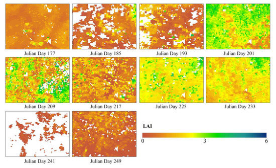
Figure 3.
Spatial distributions of MODIS LAI product.
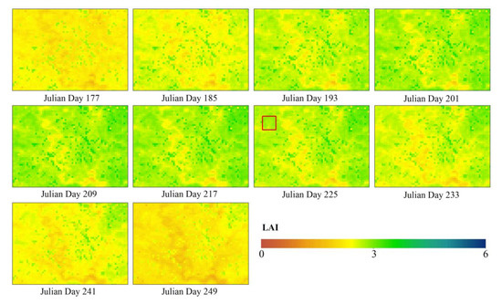
Figure 4.
Spatial distributions of the assimilated LAI values at 500 m resolution.
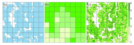
3.1.2. Spatial Distribution of Assimilated LAI at the 30 m Resolution
Compared to the 500 m resolution LAI assimilation, the assimilated LAI results at the 30 m scale (Figure 5) display a clearer seasonal green-up and senescence mode, as well as more prominent spatial distribution details and abundant texture information. Figure 6 shows an enlarged case on Julian day 225 in the red square area marked in Figure 5. The spatial distribution of crops is shown in Figure 6a. The assimilated LAI results derived from the 500 m resolution MODIS reflectance observations are illustrated in Figure 6b. They exhibit a large number of mixed pixels and low values when compared to the 30 m resolution LAI results (Figure 6c). In contrast, the spatial distributions of LAI are described in detail at the field levels (Figure 6c) through fusion of Landsat observations and the assimilated LAI results at the 500 m resolution.
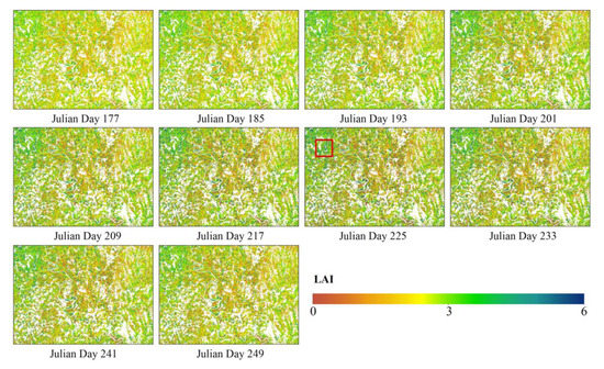
Figure 5.
Spatial distributions of assimilated LAI values at the 30 m resolution. The white parts represent the non-crop areas, such as buildings, water, and forests, etc. The red square area on Julian day 225 is enlarged in Figure 6.
3.2. Evaluation of Assimilated LAI in Time Series
Figure 7 shows the temporal profiles of various LAI estimations over four randomly selected pixels corresponding to Figure 7a–d. As can be seen from Figure 7, the original and savitsky-golay smoothed MODIS LAI tend to underestimate the reference values. Meanwhile, the MODIS LAI values from the main algorithm display the missing phenomenon during the crop growth period. Moreover, although the quality of the MODIS LAI is high for these pixels, the temporal curves of products with frequent fluctuations do not match the actual LAI variation pattern in the crop growth period. In contrast, regardless of 500 m and 30 m, the assimilated LAI profiles generated by fusing both the dynamic model and remotely sensed observations are more continuous and smoother than MODIS LAI. They remove the abrupt rises or drops from MODIS products and continuously describe the temporal changes of the LAI in crop growth season. Thus, the assimilated LAI can better depict the growth status of crops, which is in line with the law of crop phenological changes. Owing to the introduction of Landsat 8 OLI data, the assimilated results at the 30 m scale are more detailed with varying standard deviations than those from 500 m resolution. It is apparent that the assimilated LAI values perform better than MODIS LAI products when compared to the LAI references at these pixels.
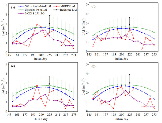
Figure 7.
Temporal comparisons of assimilated LAI results over four randomly selected pixels (a–d) including the upscaled 30 m and 500 m resolution LAI estimations, the original and savitsky-golay smoothed MODIS LAI. The mean and ±1 standard deviation values are given for the 30 m resolution assimilation and LAI references on Julian day 225.
3.3. Quantitative Evaluation of Assimilated LAI Results
At the 500 m spatial resolution, Figure 8a makes it clear that the differences between MODIS LAI products and reference LAI values are between −2.5 and 1.8 with a mean value of −0.79 and a standard deviation of 0.73, which distributes in a wide range. Moreover, the LAI differences are less than 0 over 70% of the concerned pixels. This illustrates that the MODIS LAI products contain numerous uncertainties and underestimate the LAI references. The differences between the assimilated LAI results and references range from −2 to 1.2 with a mean value of 0.46 and a standard deviation value of 0.56. A high concentration near 0 is found, indicating that the assimilated LAI values at the 500 m scale are more accurate and in better agreement with LAI reference data, when compared to the MODIS LAI products.
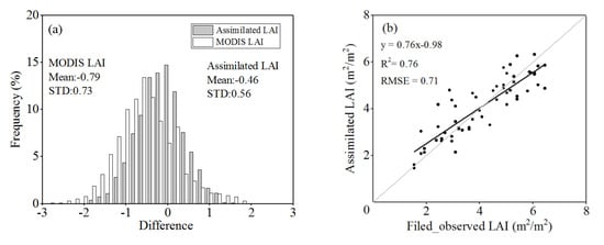
Figure 8.
Accuracy evaluation of assimilated LAI at 500 m (a) and 30 m (b) resolutions.
At the 30 m spatial resolution, a good agreement between the assimilated LAI and field measurements is observed (R2 = 0.76 and RMSE = 0.71) (Figure 8b). The scatter plots of the assimilated and field-observed LAI values basically distribute around the 1:1 line.
4. Discussion
4.1. Performance of the Proposed Method for Spatially and Temporally Continuous LAI Mapping
The spatio-temporally continuous LAI mapping from satellite observations is a popular research topic in the field of vegetation remote sensing. This study firstly constructed a LAI dynamic model based on the 500 m scale LAI assimilation for next LAI estimations at the 30 m resolution. The LAI dynamic model may result in some bias for finer resolution LAI assimilation due to the mixed effects of multiple types in the 500 m girds [22,23]. Subsequently, fine resolution LAI retrieved from Landsat 8 OLI data was used to continuously correct the 500 m scale LAI dynamic model and reconstruct the new LAI dynamics suitable for the 30 m scale study. The 30 m resolution LAI assimilations testified that the corrected LAI profiles could effectively represent the crop changes in different spatial positions and clearly describe land surface heterogeneity when compared to the 500 m resolution LAI results. Note that no missing pixels appeared in the LAI assimilation results, which exhibited high integrity, spatial continuity and discrimination, while MODIS LAI proved to be fluctuant which may be contributed to cloud contamination, the instrumentation problem and a deficient retrieval algorithm [4,5]. The proposed method provided a valuable reference for time series LAI estimations at different scale levels. It is expected that the LAI results are of significance in guiding agricultural production, formulating agricultural policies and maintaining sustainable agricultural development.
The intercomparison between multiscale LAI estimations proved that the 30 m resolution LAI values retrieved by the continuous correction algorithm through the fusion of multi-resolution remotely sensed data obtained a satisfactory accuracy (R2 = 0.76; RMSE = 0.71) and improved the expression of surface heterogeneity and the descriptions of farmland fragmentation in crop areas. [24] reported the accuracy of 30 m resolution LAI dynamics (R2 = 0.79; RMSE = 0.61) by combining 1 km MODIS LAI products and HJ CCD reflectance data through a dynamic Bayesian network. [25] showed the accuracy of the temporal high-resolution LAI (R2 = 0.80; RMSE = 0.43) through the fusion of MODIS LAI and ASTER reflectance data. Although the 500 m resolution LAI assimilation results rather than the MODIS LAI products were used to build an empirical crop growth model for LAI assimilation at the 30 m scale, the accuracy of the LAI estimations was found to be worse than the previous studies [24,25]. One main reason was that only one Landsat OLI image was used, which further limited the effectiveness of our proposed method. In contrast, 4 and 9 high-resolution images were used for LAI assimilation [24,25], respectively.
It was worthwhile to note that the temporal LAI differences between 30 m and 500 m resolution assimilations were insignificant on Julian days 201–217 when the crop LAI reached the peak value (Figure 7). This is mainly attributed to the fact that the pixels of different spatial resolutions are fully covered with crop and multiscale satellite observations consistently capture the information of homogeneous crop canopy. In contrast, the visible LAI differences are found over two spatial scales at the early and senescence stages of crop growth (e.g., Julian days 153–177, and 257–273). This may be explained by the fact that the surface reflectance data from most pixels at the 500 m resolution reflect the mixed effects of crop, soil and other types, considering that the fragmental landscape structures are serious during these periods. Furthermore, the LAI differences between the upscaled LAI reference map and the MODIS LAI products are negative over 70% of the concerned pixels (Figure 8a). That is, the MODIS LAI products underestimate the LAI references. In fact, the underestimation of MODIS LAI is universal at crop regions, which is in line with the findings of [5,10]. This phenomenon is partly attributed to the large-scale differences between coarse resolution products and actual crop fields. There is little crop field with large areas so that the 500 m pixel usually reflects the mixed signals from crop and other land cover types. At the 30 m scale (Figure 8b), the retrieved LAI from Landsat 8 OLI data was used to adjust the 500 m scale LAI dynamic model. The assimilated LAI values are easily affected by the Landsat-based LAI, especially on Julian day 225, according to the formula of the continuous correction algorithm. Most assimilated LAI values appear to be lower than the field measurements when the LAI is large. This can be explained by the fact that the spectral signal saturation cannot be certainly neglected at moderately large LAI [21]. On the other hand, most assimilated LAI values are higher than the field measurements when LAI is low, which is associated with the characteristics of the LAI retrieved from Landsant OLI.
4.2. Limitations of this Study and Prospects for Future Studies
Currently, the acquisitions of fine resolution optical images are seriously limited due to the revisit period of satellite sensors and adverse weather conditions (e.g., cloud), especially over southwestern China. In this study, only one Landsat 8 OLI reflectance image was acquired during the crop growing season, which might decrease the positive roles of the continuous correction assimilation algorithm. The integration of data from multisource sensors can compensate for the data deficiency of a single sensor for the LAI estimations at high spatio-temporal resolutions [38,39,40]. At present, several high-resolution optical sensors, such as Sentinel-2, GF and SPOT, provide multiple observations with different revisit periods during crop growth seasons. More importantly, a mixture of optical and microwave sensors increases the frequency of usable satellite data. Further study will reconstruct the complementary satellite dataset from multisource sensors for high resolution LAI retrievals. In addition, the image fusion schemes, such as STARFM [41] and ESTARFM [42], overcome the contradiction between spatial and temporal resolutions of different sensors to derive the surface reflectance data at fine spatio-temporal resolution levels. These reflectance data can be adopted to estimate high spatial and temporal resolution LAI with the help of data assimilation algorithms in future researches.
It should be noted that only the temporal LAI dynamics was integrated into the current data assimilation process in the present study, while other vegetation parameters (e.g., ALA, Cab, Cm) used in the PROSAIL model may possess inherent temporal change laws. The lack of temporal information for these parameters except the LAI still brings uncertainties for the time series LAI assimilation. Therefore, one potential future-research priority should focus on the integration of temporal profiles of the multiple biophysical variables and multisource remotely sensed observations to improve the accuracy of the time series LAI estimations.
5. Conclusions
The spatially and temporally continuous LAI mapping at the 500 m and 30 m scales were achieved with the help of the VFSA and continuous correction assimilation algorithms. Compared to MODIS LAI products, the assimilated LAI results at the 500 m scale showed better spatial integrity and temporal continuity. The proposed method was feasible and effective to solve the spatio-temporal discontinuities of the existing LAI products and improved the accuracy of coarse resolution LAI retrievals. The LAI maps at the 30 m scale represented the characteristics of spatial heterogeneity of farmlands in fragile areas and generated good consistency with the corresponding field LAI measurements (R2 = 0.76, RMSE = 0.71). Furthermore, the temporal profiles of LAI at the 30 m scale captured the gradual changes of the LAI in the time series and reasonably described the crop growth process. The comparisons of the temporal LAI profiles between the 30 m and 500 m resolutions showed the change of spatial heterogeneity with time in different crop growth stages.
The multi-stage data assimilation strategy in this study not only offered a methodology to downscale coarse resolution LAI products, but also provided a good reference for fine resolution retrievals of other biophysical parameters (e.g., the fraction of absorbed photosynthetically active radiation and fraction of vegetation cover) from multiresolution satellite images. More importantly, this study fills the gap in fine resolution LAI retrievals in the time series over fragmented areas, which is particularly important for supporting precise farming activities in these regions.
Author Contributions
Data curation, H.X.; Funding acquisition, A.L.; Investigation, Z.Z.; Methodology, H.J.; Resources, H.J.; Validation, X.X.; Writing—original draft, W.X.; Writing—review & editing, H.J.
Funding
This research was funded by National Natural Science Foundation of China (Grant No. 41671376, 41631180, 41301385), Sichuan Science and Technology Program (Grant No. 2019YJ0007), National Key Research and Development Program of China (Grant No. 2016YFA0600103) and Open Fund of Key Laboratory of Geospatial Technology for the Middle and Lower Yellow River Regions (Henan University), Ministry of Education (Grant No. GTYR201802).
Acknowledgments
We are grateful to the anonymous reviewers for their valuable comments and suggestions.
Conflicts of Interest
The authors declare no conflict of interest.
References
- Dente, L.; Satalino, G.; Mattia, F.; Rinaldi, M. Assimilation of leaf area index derived from ASAR and MERIS data into CERES-Wheat model to map wheat yield. Remote Sens. Environ. 2008, 112, 1395–1407. [Google Scholar] [CrossRef]
- Huang, J.; Ma, H.; Sedano, F.; Lewis, P.; Liang, S.; Wu, Q.; Su, W.; Zhang, X.; Zhu, D. Evaluation of regional estimates of winter wheat yield by assimilating three remotely sensed reflectance datasets into the coupled WOFOST-PROSAIL model. Eur. J. Agron. 2019, 102, 1–13. [Google Scholar] [CrossRef]
- Ma, G.; Huang, J.; Wu, W.; Fan, J.; Zou, J.; Wu, S. Assimilation of MODIS-LAI into the WOFOST model for forecasting regional winter wheat yield. Math. Comput. Model. 2013, 58, 634–643. [Google Scholar] [CrossRef]
- Fang, H.; Jiang, C.; Li, W.; Wei, S.; Baret, F.; Chen, J.M.; Garcia-Haro, J.; Liang, S.; Liu, R.; Myneni, R.B.; et al. Characterization and intercomparison of global moderate resolution leaf area index (LAI) products: Analysis of climatologies and theoretical uncertainties. J. Geophys. Res. Biogeosci. 2013, 118, 529–548. [Google Scholar] [CrossRef]
- Jin, H.; Li, A.; Bian, J.; Nan, X.; Zhao, W.; Zhang, Z.; Yin, G. Intercomparison and validation of MODIS and GLASS leaf area index (LAI) products over mountain areas: A case study in southwestern China. Int. J. Appl. Earth Obs. Geoinf. 2017, 55, 52–67. [Google Scholar] [CrossRef]
- Chen, J.M.; Black, T.A. Defining leaf area index for non-flat leaves. Plant Cell Environ. 1992, 15, 421–429. [Google Scholar] [CrossRef]
- Knyazikhin, Y.; Martonchik, J.V.; Myneni, R.B.; Diner, D.J.; Running, S.W. Synergistic algorithm for estimating vegetation canopy leaf area index and fraction of absorbed photosynthetically active radiation from MODIS and MISR data. J. Geophys. Res. Space Phys. 1998, 103, 32257–32275. [Google Scholar] [CrossRef]
- Xiao, Z.; Liang, S.; Wang, J.; Xiang, Y.; Zhao, X.; Song, J. Long-Time-Series Global Land Surface Satellite Leaf Area Index Product Derived from MODIS and AVHRR Surface Reflectance. IEEE Trans. Geosci. Remote Sens. 2016, 54, 1–18. [Google Scholar] [CrossRef]
- Baret, F.; Weiss, M.; Lacaze, R.; Camacho, F.; Makhmara, H.; Pacholcyzk, P.; Smets, B. GEOV1: LAI and FAPAR essential climate variables and FCOVER global time series capitalizing over existing products. Part1: Principles of development and production. Remote Sens. Environ. 2013, 137, 299–309. [Google Scholar] [CrossRef]
- Fang, H.; Wei, S.; Liang, S. Validation of MODIS and CYCLOPES LAI products using global field measurement data. Remote Sens. Environ. 2012, 119, 43–54. [Google Scholar] [CrossRef]
- Gessner, U.; Niklaus, M.; Kuenzer, C.; Dech, S. Intercomparison of Leaf Area Index Products for a Gradient of Sub-Humid to Arid Environments in West Africa. Remote Sens. 2013, 5, 1235–1257. [Google Scholar] [CrossRef]
- Xu, B.; Li, J.; Park, T.; Liu, Q.; Zeng, Y.; Yin, G.; Zhao, J.; Fan, W.; Yang, L.; Knyazikhin, Y.; et al. An integrated method for validating long-term leaf area index products using global networks of site-based measurements. Remote Sens. Environ. 2018, 209, 134–151. [Google Scholar] [CrossRef]
- Gao, F.; Anderson, M.C.; Kustas, W.P.; Houborg, R. Retrieving Leaf Area Index from Landsat Using MODIS LAI Products and Field Measurements. IEEE Geosci. Remote Sens. Lett. 2014, 11, 773–777. [Google Scholar]
- Hernández, C.; Nunes, L.; Lopes, D.; Graña, M. Data fusion for high spatial resolution LAI estimation. Inf. Fusion 2014, 16, 59–67. [Google Scholar] [CrossRef]
- Houborg, R.; McCabe, M.F.; Gao, F. A Spatio-Temporal Enhancement Method for medium resolution LAI (STEM-LAI). Int. J. Appl. Earth Obs. Geoinf. 2016, 47, 15–29. [Google Scholar] [CrossRef]
- Wu, M.; Wu, C.; Huang, W.; Niu, Z.; Wang, C. High-resolution Leaf Area Index estimation from synthetic Landsat data generated by a spatial and temporal data fusion model. Comput. Electron. Agric. 2015, 115, 1–11. [Google Scholar] [CrossRef]
- Senf, C.; Leitão, P.J.; Pflugmacher, D.; Van Der Linden, S.; Hostert, P. Mapping land cover in complex Mediterranean landscapes using Landsat: Improved classification accuracies from integrating multi-seasonal and synthetic imagery. Remote Sens. Environ. 2015, 156, 527–536. [Google Scholar] [CrossRef]
- Zhu, X.; Helmer, E.H.; Gao, F.; Liu, D.; Chen, J.; Lefsky, M.A. A flexible spatiotemporal method for fusing satellite images with different resolutions. Remote Sens. Environ. 2016, 172, 165–177. [Google Scholar] [CrossRef]
- Reichle, R.H. Data assimilation methods in the Earth sciences. Adv. Water Resour. 2008, 31, 1411–1418. [Google Scholar] [CrossRef]
- Huang, J.; Sedano, F.; Huang, Y.; Ma, H.; Li, X.; Liang, S.; Tian, L.; Zhang, X.; Fan, J.; Wu, W. Assimilating a synthetic Kalman filter leaf area index series into the WOFOST model to improve regional winter wheat yield estimation. Agric. For. Meteorol. 2016, 216, 188–202. [Google Scholar] [CrossRef]
- Jin, H.; Li, A.; Yin, G.; Xiao, Z.; Bian, J.; Nan, X.; Jing, J. A Multiscale Assimilation Approach to Improve Fine-Resolution Leaf Area Index Dynamics. IEEE Trans. Geosci. Remote Sens. 2019, 57, 8153–8168. [Google Scholar] [CrossRef]
- Jin, H.A.; Li, A.N.; Wang, J.D.; Bo, Y.C. Improvement of spatially and temporally continuous crop leaf area index by integration of CERES-Maize model and MODIS data. Eur. J. Agron. 2016, 78, 1–12. [Google Scholar] [CrossRef]
- Zhang, Y.; Qu, Y.; Wang, J.; Liang, S.; Liu, Y. Estimating leaf area index from MODIS and surface meteorological data using a dynamic Bayesian network. Remote Sens. Environ. 2012, 127, 30–43. [Google Scholar] [CrossRef]
- Qu, Y.; Zhang, Y.; Xue, H. Retrieval of 30 m resolution leaf area index from China HJ-1 CCD data and MODIS products through a dynamic bayesian network. IEEE J. Sel. Top. Appl. Earth Obs. Remote Sens. 2014, 7, 222–228. [Google Scholar]
- Qu, Y.; Han, W.; Ma, M. Retrieval of a temporal high-resolution leaf area index (LAI) by combining MODIS LAI and ASTER reflectance data. Remote Sens. 2015, 7, 195–210. [Google Scholar] [CrossRef]
- Pisek, J.; Chen, J.M.; Lacaze, R.; Sonnentag, O.; Alikas, K. Expanding global mapping of the foliage clumping index with multi-angular POLDER three measurements: Evaluation and topographic compensation. ISPRS J. Photogramm. Remote Sens. 2010, 65, 341–346. [Google Scholar] [CrossRef]
- Myneni, R.B.; Hoffman, S.; Knyazikhin, Y.; Privette, J.L.; Glassy, J.; Tian, Y.; Wang, Y.; Song, X.; Zhang, Y.; Smith, G.R.; et al. Global products of vegetation leaf area and fraction absorbed PAR from year one of MODIS data. Remote Sens. Environ. 2002, 83, 214–231. [Google Scholar] [CrossRef]
- Li, A.; Lei, G.; Zhang, Z.; Bian, J.; Deng, W. China land cover monitoring in mountainous regions by remote sensing technology Taking the Southwestern China as a case. In Proceedings of the IEEE Geoscience and Remote Sensing Symposium, Quebec City, QC, Canada, 13–18 July 2014; pp. 4216–4219. [Google Scholar]
- Jacquemoud, S.; Baret, F. Prospect: A model of leaf optical properties spectra. Remote Sens. Environ. 1990, 34, 75–91. [Google Scholar] [CrossRef]
- Verhoef, W. Light scattering by leaf layers with application to canopy reflectance modeling: The SAIL model. Remote Sens. Environ. 1984, 16, 125–141. [Google Scholar] [CrossRef]
- Jacquemoud, S.; Verhoef, W.; Baret, F.; Bacour, C.; Zarco-Tejada, P.J.; Asner, G.P.; François, C.; Ustin, S.L. PROSPECT + SAIL models: A review of use for vegetation characterization. Remote Sens. Environ. 2009, 113, 56–66. [Google Scholar] [CrossRef]
- Li, X.; Koike, T.; Pathmathevan, M. A very fast simulated re-annealing (VFSA) approach for land data assimilation. Comput. Geosci. 2004, 30, 239–248. [Google Scholar] [CrossRef]
- Salinas, S.V.; Chang, C.W.; Liew, S.C. Multiparameter retrieval of water optical properties from above-water remote-sensing reflectance using the simulated annealing algorithm. Appl. Opt. 2007, 46, 2727–2742. [Google Scholar] [CrossRef] [PubMed]
- Wang, J.; Li, X.; Lu, L.; Fang, F. Estimating near future regional corn yields by integrating multi-source observations into a crop growth model. Eur. J. Agron. 2013, 49, 126–140. [Google Scholar] [CrossRef]
- Dong, Y.Y.; Zhao, C.J.; Yang, G.J.; Chen, L.P.; Wang, J.H.; Feng, H.K. Integrating a very fast simulated annealing optimization algorithm for crop leaf area index variational assimilation. Math. Comput. Model. 2013, 58, 871–879. [Google Scholar] [CrossRef]
- Wan, H.; Wang, J.; Xiao, Z.; Li, L. Generating the high spatial and temporal resolution LAI by fusing MODIS and ASTER. J. Beijing Norm. Univ. Nat. Sci. 2007, 43, 303–308. [Google Scholar]
- Weiss, M.; Baret, F.; Garrigues, S.; Lacaze, R. LAI and fAPAR CYCLOPES global products derived from VEGETATION. Part 2: Validation and comparison with MODIS collection 4 products. Remote Sens. Environ. 2007, 110, 317–331. [Google Scholar] [CrossRef]
- Campos-Taberner, M.; García-Haro, F.J.; Camps-Valls, G.; Grau-Muedra, G.; Nutini, F.; Crema, A.; Boschetti, M. Multitemporal and multiresolution leaf area index retrieval for operational local rice crop monitoring. Remote Sens. Environ. 2016, 187, 102–118. [Google Scholar] [CrossRef]
- Gray, J.; Song, C. Mapping leaf area index using spatial, spectral, and temporal information from multiple sensors. Remote Sens. Environ. 2012, 119, 173–183. [Google Scholar] [CrossRef]
- Liu, Q.; Liang, S.; Xiao, Z.; Fang, H. Retrieval of leaf area index using temporal, spectral, and angular information from multiple satellite data. Remote Sens. Environ. 2014, 145, 25–37. [Google Scholar] [CrossRef]
- Gao, F.; Masek, J.; Schwaller, M.; Hall, F. On the blending of the Landsat and MODIS surface reflectance: predicting daily Landsat surface reflectance. IEEE Trans. Geosci. Remote Sens. 2006, 44, 2207–2218. [Google Scholar]
- Zhu, X.; Chen, J.; Gao, F.; Chen, X.; Masek, J.G. An enhanced spatial and temporal adaptive reflectance fusion model for complex heterogeneous regions. Remote Sens. Environ. 2010, 114, 2610–2623. [Google Scholar] [CrossRef]


© 2019 by the authors. Licensee MDPI, Basel, Switzerland. This article is an open access article distributed under the terms and conditions of the Creative Commons Attribution (CC BY) license (http://creativecommons.org/licenses/by/4.0/).