Evaluating Resilience-Centered Development Interventions with Remote Sensing

Abstract

Natural disasters are projected to increase in number and severity, in part due to climate change. At the same time a growing number of disaster risk reduction (DRR) and climate change adaptation measures are being implemented by governmental and non-governmental organizations, and substantial post-disaster donations are frequently pledged. At the same time there has been increasing demand for transparency and accountability, and thus evidence of those measures having a positive effect. We hypothesized that resilience-enhancing interventions should result in less damage during a hazard event, or at least quicker recovery. In this study we assessed recovery over a 3 year period of seven municipalities in the central Philippines devastated by Typhoon Haiyan in 2013. We used very high resolution optical images (<1 m), and created detailed land cover and land use maps for four epochs before and after the event, using a machine learning approach with extreme gradient boosting. The spatially and temporally highly variable recovery maps were then statistically related to detailed questionnaire data acquired by DEval in 2012 and 2016, whose principal aim was to assess the impact of a 10 year land-planning intervention program by the German agency for technical cooperation (GIZ). The survey data allowed very detailed insights into DRR-related perspectives, motivations and drivers of the affected population. To some extent they also helped to overcome the principal limitation of remote sensing, which can effectively describe but not explain the reasons for differential recovery. However, while a number of causal links between intervention parameters and reconstruction was found, the common notion that a resilient community should recover better and more quickly could not be confirmed. The study also revealed a number of methodological limitations, such as the high cost for commercial image data not matching the spatially extensive but also detailed scale of field evaluations, the remote sensing analysis likely overestimating damage and thus providing incorrect recovery metrics, and image data catalogues especially for more remote communities often being incomplete. Nevertheless, the study provides a valuable proof of concept for the synergies resulting from an integration of socio-economic survey data and remote sensing imagery for recovery assessment.

1. Introduction

The average annual global economic damage caused by disasters is difficult to determine, with estimations ranging from about 300 billion US$ [1,2] to more than 520 billion US$ [3]. Predictions of future damages, in particular as part of wider expected losses resulting from climate change, are even harder, with different warming scenarios by the Intergovernmental Panel on Climate Change (IPCC) leading to a wide range of consequences [4], including variable changes in hydrometeorological hazards [5]. Nevertheless, it is widely accepted that economic consequences will be both severe and spatially highly variable [6,7]. Substantial uncertainty in those predictions is linked to the likely extent and effect of climate change adaptation (CCA) and disaster risk reduction (DRR) measures. The United Nations Environment Programme (UNEP) [8] recently estimated annual CCA costs of up to 500 billion US$. Vast sums have already been pledged for such measures by both governmental and non-governmental players. The European Union announced plans in the 2009 Copenhagen Accord to invest 100 billion US$ annually by 2020 in CCA measures in developing countries. In addition, the work plan of virtually every official development assistance (ODA) agency includes a wide array of interventions to reduce disaster risk and the effects of climate change, aiming at fostering greater resilience.

A greater challenge than carrying out those interventions, be it engineering measures to protect coastal communities, efforts to support the development of comprehensive land use plans, or to work with local non-governmental organizations (NGO) to build up community-level risk awareness, is to assess their effect. In particular with the increase in spending on development cooperation, politicians are under pressure to demonstrate that the money is spent effectively. Therefore, evaluation has become an important tool to demonstrate that tax-payer money is used wisely and that programs have a positive impact [9]. For example, it stands to reason that communities that have received several years of DRR interventions should suffer less damage during a hazard event, or at least recover more quickly than unassisted communities. However, assessing the effect of interventions is complicated. This is because of the difficulty (i) to attribute a certain performance or behavior of people or governments to specific interventions, especially when different organizations are active in the area, (ii) to estimate the future effect and value of planning activities or what people learned in a community meeting, and (iii) to collect the very detailed socio-economic data needed to support a quantitative impact evaluation. CCA and DRR are only two domains where the need for impact assessment has been increasing. There has generally been growing interest in transparency and accountability, with auditing agencies but also donors giving post-disaster assistance increasingly requesting evidence of the effect of funded interventions.

Impact evaluations, which can address relevance, effectiveness, efficiency, impact, or sustainability, usually follow a common procedure: first, evaluators collect baseline data prior to the start of the intervention. After the program has been completed and project impacts have crystalized endline data are compiled. It is good practice to collect additional performance data during the program implementation stage to carry out adjustments if needed. Data collection is performed in treatment and non-treatment communities. Ideally treatment is assigned randomly (randomized control trial), but if this is not possible, matching methods can be employed (quasi-experimental design) [9].

In the field of international development the focus is primarily on people. As such, surveys are the most frequently used tool for data collection. Often survey data are amended with socio-economic and demographic characteristics of the region to contextualize findings. These additional data are usually obtained from census records made available by Integrated Public Use Microdata Series (IPUMS)-International [10], or via specialized population surveys such as the demographic and health surveys [11]. Based on the nature of the data, the evaluation design, and the outcome of interest, different statistical models can be employed to connect treatment with impacts causally. The statistical tests range from simple t-tests to more complex multi-level regression models [12]. However, most traditional evaluations in the field of international development cooperation do not consider space. With advances in spatial technology, evaluators have now started to employ geographic data in evaluations [13,14]. Geographic parameters can be employed either as control or outcome variables, or in the evaluation design stage such as for spatial sampling. When the program impact is measured geographically it is possible to employ a geospatial impact evaluation (GIE) approach [15].

Traditional impact evaluation methods face a number of limitations: (i) collecting survey data is a time consuming and expensive task [9]. Particularly if a program is implemented widely across a country or region, costs can rise drastically and limit either coverage or detail; (ii) traditional survey methods require a long planning horizon and are difficult to implement ad-hoc. This makes it challenging to collect baseline data for programs that respond to sudden onset disasters such as storms, flooding, or earthquakes [14]; (iii), traditional survey methods are restricted by access considerations. For example, it is difficult to evaluate programs that take place in very remote locations without proper road access. Similarly, the political situation in a country (e.g., military conflict) may prevent evaluators from collecting survey information [16].

The advantages of remote sensing (RS) in terms of synoptic coverage, cost effectiveness, and flexibility in sampling frequency or sensor choice are well recognized in the field of disaster risk management [17]. However, most image analysis methods developed in this domain focus on the detection or characterization of physical features. Only more recent research has also looked at non-physical properties such as social vulnerability [18] or functional disaster damage. All make use of physical proxy indicators (hereafter: proxies) constituting indirect measures that provide insights into not directly observable features or processes [19].

The purpose of this study was to understand to what extent RS could support the traditionally field-based evaluation work. Specifically, we focused on assessing the effect of interventions on resilience, i.e., the ability to rebound from an adverse event. We considered post-disaster recovery to be a proxy for resilience, and thus used RS to detect evidence of spatially variable recovery, which we then statistically linked to interventions in different municipalities. Similar to [20] we assessed land cover (LC) and land use (LU) with machine learning (ML) methods over a 3 year period following a disaster event to detect the level of recovery across space, which was then related to intervention information collected in the field. We developed the proof of concept for a number of barangays (municipalities) in the Leyte region in the central Philippines, which was severely affected during Typhoon Haiyan in 2013.

2. Literature Review and State of the Art

In a political climate of increasing calls for transparency and accountability, evaluations can provide empirical evidence of intervention effectiveness, efficiency, and impact to justify spending. To be able to estimate the causal effect or impact of a program, evaluations must estimate the counterfactual, i.e., what the outcome would have been in the absence of the program [9]. It is the goal to control for all factors that may have produced the results, and thereby clearly connect intervention and outcome.

Impact evaluations employ different methods to estimate a valid counterfactual, including randomized assignment [21], regression discontinuity [22], difference-in-difference [23], and matching [24]. Given a sufficiently large sample, randomized assignment ensures that the treatment and control groups are statistically identical in both observed and unobserved characteristics [25]. Regression discontinuity design is an option when a continuous scale (e.g., poverty index, and farm size) is used to determine program eligibility, and a unique cutoff score determines who receives the program [26]. It is then possible to calculate impacts as the difference in outcomes comparing the units just below (e.g., treatment group) and above (e.g., control group) the eligibility cutoff. The difference-in-difference method compares changes in the outcome (before and after the intervention) of the treatment group with changes in the outcome of the comparison group [27]. Matching belongs to the category of quasi-experimental designs and uses statistical methods to find for every treatment unit a non-treatment unit that has the most similar characteristics possible [28]. However, when experimental and quasi-experimental designs are unethical or not feasible, evaluators frequently employ correlation methods (e.g., multivariate regressions) to account statistically for differences between treatment and control units [29]. In this paper, we employed a correlation approach to investigate the impact of a land-use planning intervention (see details below) on post-disaster recovery, and thus on resilience.

A prerequisite for employing rigorous evaluation methodologies is sufficient data availability. Traditionally, evaluations have made use of survey methods to collect the necessary data before, during and after an intervention. However, the collection of survey data is expensive and responses may be subjective. In addition, survey data frequently lack the geographical detail if environmental changes are to be evaluated [13]. The use of RS data to complement traditional evaluation designs offers some major advantages [30], such as archives that often span decades, and thus the availability of image data acquired long before the intervention started. Many satellite products are available free of charge, which may help reduce the costs for data collection. Finally, geographic data can provide an objective measure of high detail for changes in environmental conditions, which is difficult to obtain from survey data alone.

Many methods have been developed to extract information from RS data to measure and characterize different aspects of disaster risk management [17,31]. However, most existing studies have focused on physical assessments using direct observations, be it for hazard or risk assessment, but also to detect post-disaster damage or recovery. For example, researchers have assessed the number of buildings collapsed/damaged [32,33] and reconstructed [34], or estimated their vulnerability [35]. However, the non-physical aspects of DRM, e.g., social and economic properties, are also crucial and should be assessed [36]. However, this requires indirect observations and the use of proxies [19], as demonstrated in recent studies on vulnerability [37,38], resilience [39], damage [40,41], and recovery [42]. In addition, recent studies showed that most of the developed proxies for damage and recovery assessments can be extracted through LC and LU monitoring [43,44], increasingly through the use of ML techniques [20]. The growing sophistication of image-based extraction of both physical and non-physical indicators of recovery, and thus resilience, suggests a possible role in impact evaluation, which we tested in this work.

3. Data and Methods

3.1. Overall Approach

Figure 1 illustrates the overall methodological approach followed in this study. Using a variety of image-derived proxies that cover the built-up, social, and economic dimensions we first quantified the damage caused by typhoon Haiyan, followed by a quantification of the recovery for different post-event years. The spatially variable recovery performance was considered to reflect the underlying resilience. In a statistical analysis we then identified which intervention-related variables, such as donor support, but also factors such as prior disaster experience, correlated with the observed recovery at a municipal level.

In the following we first provide details about the study area and the satellite data used, as well as the field surveys carried out by the German Institute for Development Evaluation (DEval). Subsequently we explained the developed proxies, and how they were used in the damage and recovery assessment. Finally the correlation analysis to link the RS results and the impact evaluation data was described.

3.2. Study Location and Image Data Used

Typhoon Haiyan passed over the Central Visayas region of the Philippines, crossing the islands of Samar and Leyte on 8 November 2013. With sustained wind speeds exceeding 310 km/h at landfall, it was one of the strongest tropical storms on record worldwide. The center of the storm passed close to Leyte’s largest city and administrative center, Tacloban (Figure 2).

Reported fatality figures vary widely, though are unofficially estimated to be in excess of 13,000 [45] attributable to strong winds and a storm surge of up to 5 m in height along the Basey and Tacloban coastal area [46]. Other sources reported heights of up to 7 m in Leyte [47], and even 12 m in Samar [48]. Structural damage was extensive, with more than 1 million buildings getting partially or completely destroyed in nearly 600 affected municipalities. Leyte alone accounted for a reported 86% of all casualties, and a quarter of the economic losses relate to destroyed rice and corn crops [49].

Very high-resolution satellite images were used to implement the developed LCLU classification approach and to extract relevant proxies.

Table 1. Satellite images used in this study.

Area	Satellite	Acquisition Date	Time (T0, T1, T2, T3) 1	Spatial Resolution 2 (MS; Pan)
Tacloban	WorldView2	2013-03-17	T0	2 m; 0.5 m
Tacloban	WorldView2	2017-03-18	T3	2 m; 0.5 m
Tacloban	GeoEye1	2013-11-10	T1	2 m; 0.5 m
Tacloban	GeoEye1	2013-11-12	T1	2 m; 0.5 m
Tacloban	GeoEye1	2013-11-13	T1	2 m; 0.5 m
Tacloban	GeoEye1	2016-04-24	T2	2 m; 0.5 m
South Leyte	WorldView2	2013-03-25	T0	2 m; 0.5 m
South Leyte	WorldView2	2013-04-02	T0	2 m; 0.5 m
South Leyte	WorldView2	2014-01-07	T1	2 m; 0.5 m
South Leyte	WorldView2	2014-07-16	T2	2 m; 0.5 m
South Leyte	WorldView2	2014-09-11	T2	2 m; 0.5 m
South Leyte	WorldView2	2014-10-21	T2	2 m; 0.5 m
South Leyte	WorldView2	2014-12-01	T2	2 m; 0.5 m
South Leyte	WorldView2	2016-01-24	T3	2 m; 0.5 m
South Leyte	WorldView2	2016-06-24	T3	2 m; 0.5 m
Basey	WorldView2	2013-05-18	T0	2 m; 0.5 m
Basey	WorldView2	2013-05-18	T0	2 m; 0.5 m
Basey	WorldView2	2013-09-01	T0	2 m; 0.5 m
Basey	WorldView2	2013-11-19	T1	2 m; 0.5 m
Basey	WorldView2	2013-11-21	T1	2 m; 0.5 m
Basey	WorldView3	2014-12-09	T2	1.3 m; 0.31 m
Basey	WorldView3	2015-01-10	T2	1.3 m; 0.31 m
Basey	WorldView2	2016-06-04	T3	2 m; 0.5 m
Basey	WorldView2	2016-06-04	T3	2 m; 0.5 m
Lawaan	WorldView2	2013-05-18	T0	2 m; 0.5 m
Lawaan	WorldView2	2013-05-18	T0	2 m; 0.5 m
Lawaan	WorldView2	2014-01-07	T1	2 m; 0.5 m
Lawaan	WorldView2	2014-01-07	T1	2 m; 0.5 m
Lawaan	WorldView3	2014-10-07	T2	1.3 m; 0.31 m
Lawaan	WorldView2	2015-11-24	T3	2 m; 0.5 m

¹ T0—pre-disaster, T1—shortly after Haiyan, T2 and T3—approx. 2 years and 3 years after the disaster, respectively. ² MS—multispectral, Pan—panchromatic.

shows the specifications and acquisition times of the images used.

3.3. Survey Data

To test the integration of survey information with RS data we selected seven municipalities that were part of a larger evaluation completed by DEval [14]. The evaluation included 100 municipalities, of which 44 formed the intervention group, and 56 the control group. Control municipalities were selected from all available municipalities in the two study regions (Eastern Visayas and Western Visayas) using a propensity-score matching technique [50]. Base- and endline survey data were collected by DEval for 10 households in three randomly selected barangays per municipality, resulting in 3000 interviewed households.

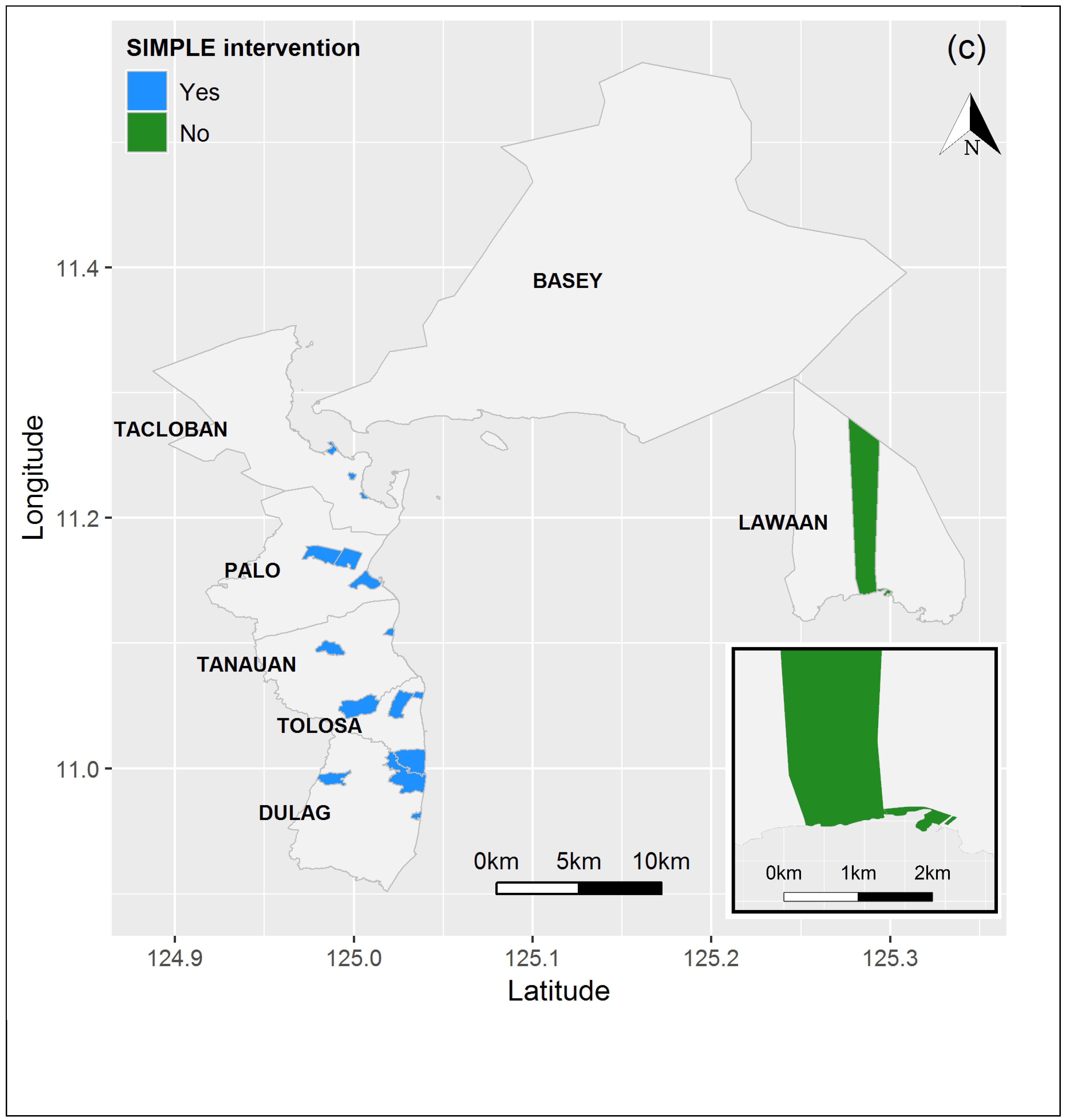
The intervention evaluated by DEval was a comprehensive LU planning program known as SIMPLE (Sustainable Integrated Management and Planning for Local Government Ecosystems) that received funding and administrative support from the German agency for technical cooperation (GIZ) over a 10-year period (2006–2015). The SIMPLE intervention included training schemes, technical assistance, and the development of participatory planning tools. The DEval evaluation found that the SIMPLE intervention significantly improved land-use planning quality and comprehensiveness, and led to an increased number of protected areas [14]. The DEval evaluation investigated the general effectiveness of the SIMPLE intervention on land-use planning approaches in the Philippines but did not evaluate post-disaster recovery, the focus of this article.

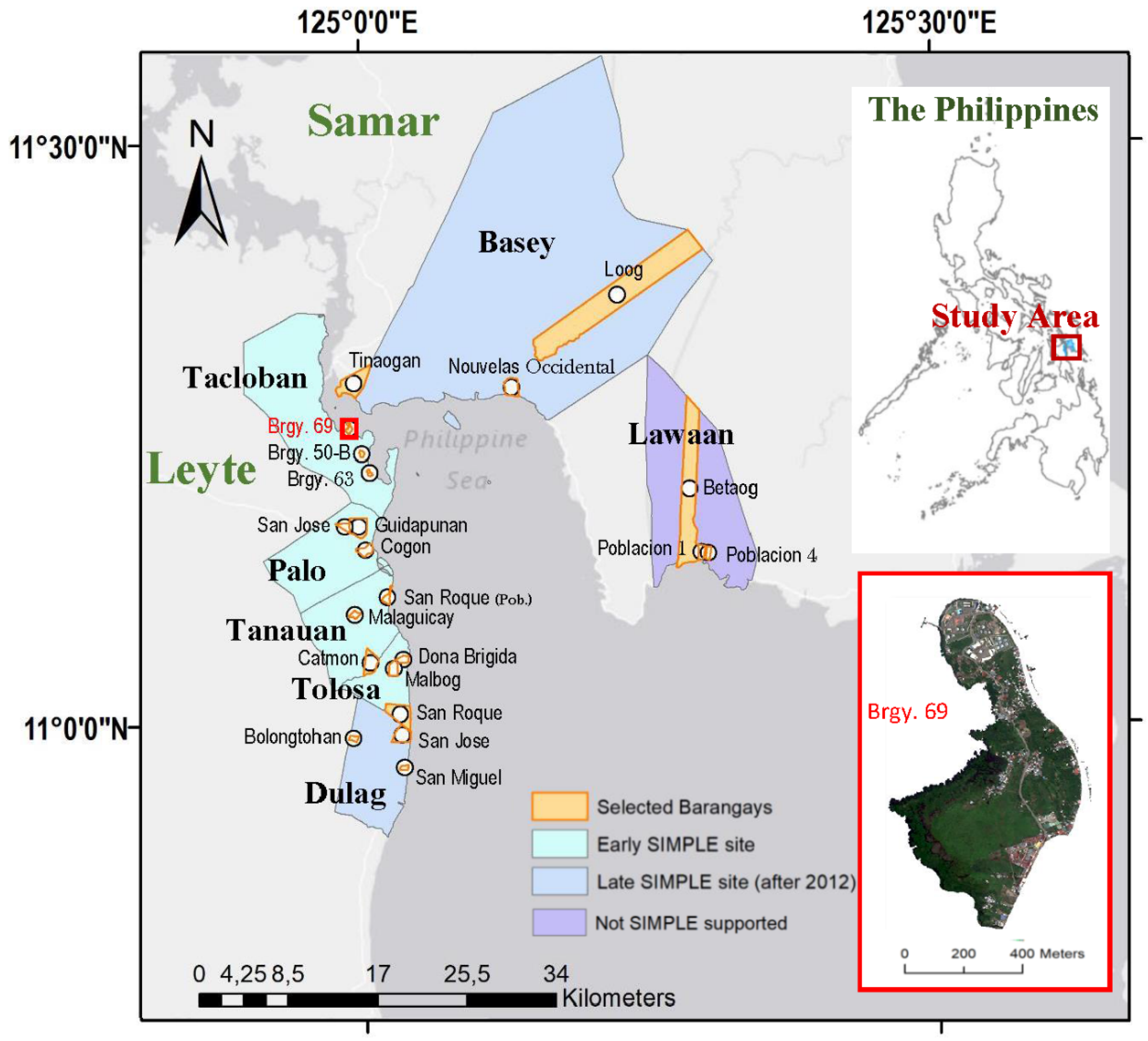
During the DEval impact evaluation extensive panel survey data were collected at the household, barangay, and municipal levels. Base- and endline data were collected in 2012 and 2016, respectively. Due to budget constraints we were unable to perform the remote sensing analysis for all surveyed municipalities for the study reported in this paper. The seven municipalities were purposefully chosen for two reasons: (i) we selected municipalities that were affected to different degrees by Haiyan, to capture sufficient variation in damage and recovery; and (ii) we further ensured that both treated (receipt of SIMPLE intervention) and untreated municipalities were represented in our sample. From each of the seven municipalities three barangays (villages) were randomly selected, resulting in a sample of N = 21 barangays. However, data limitations (e.g., cloud coverage in some of the RS data) led to a reduction in the analytic sample to N between 13–18, depending on the geographic variable. 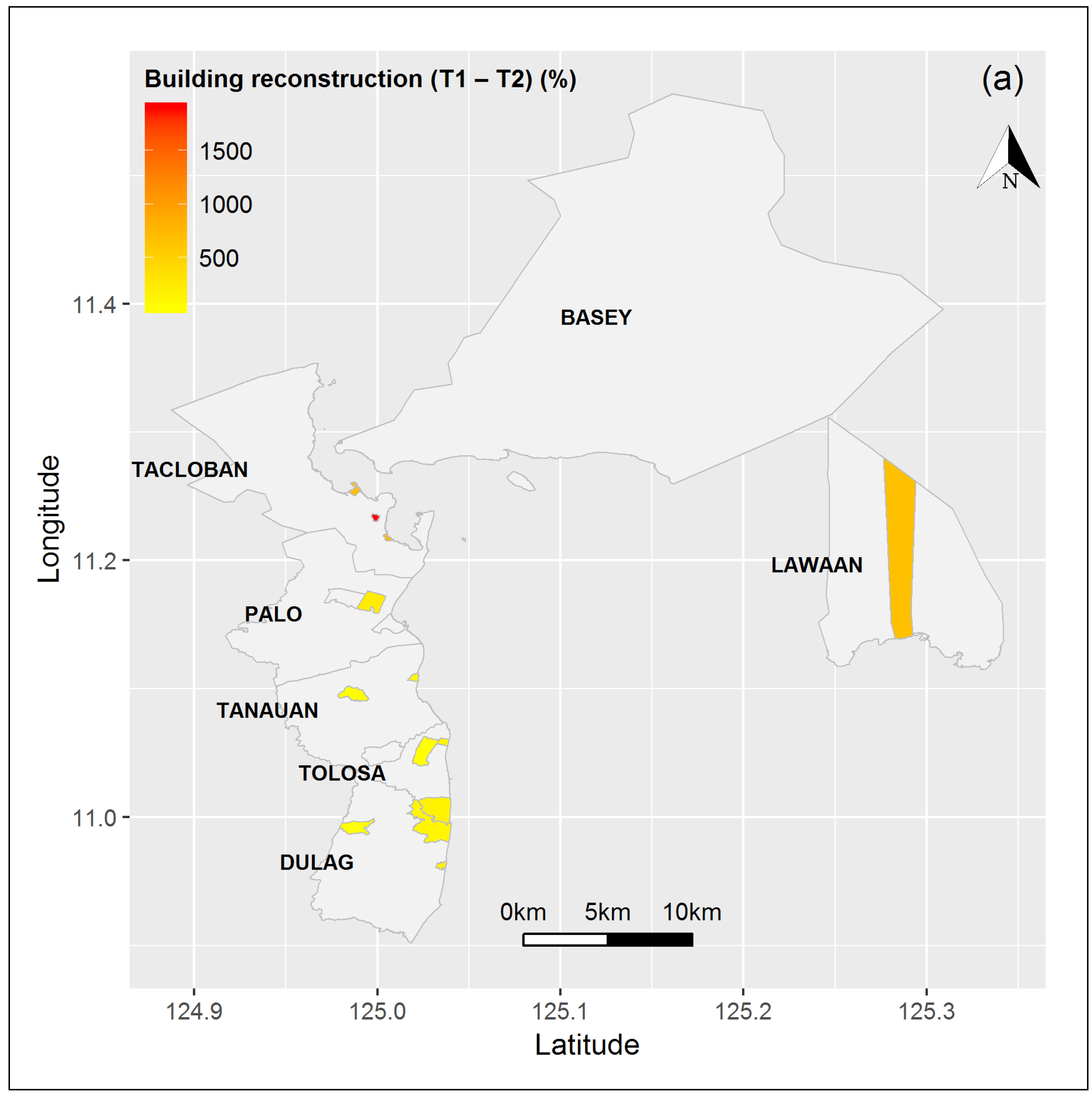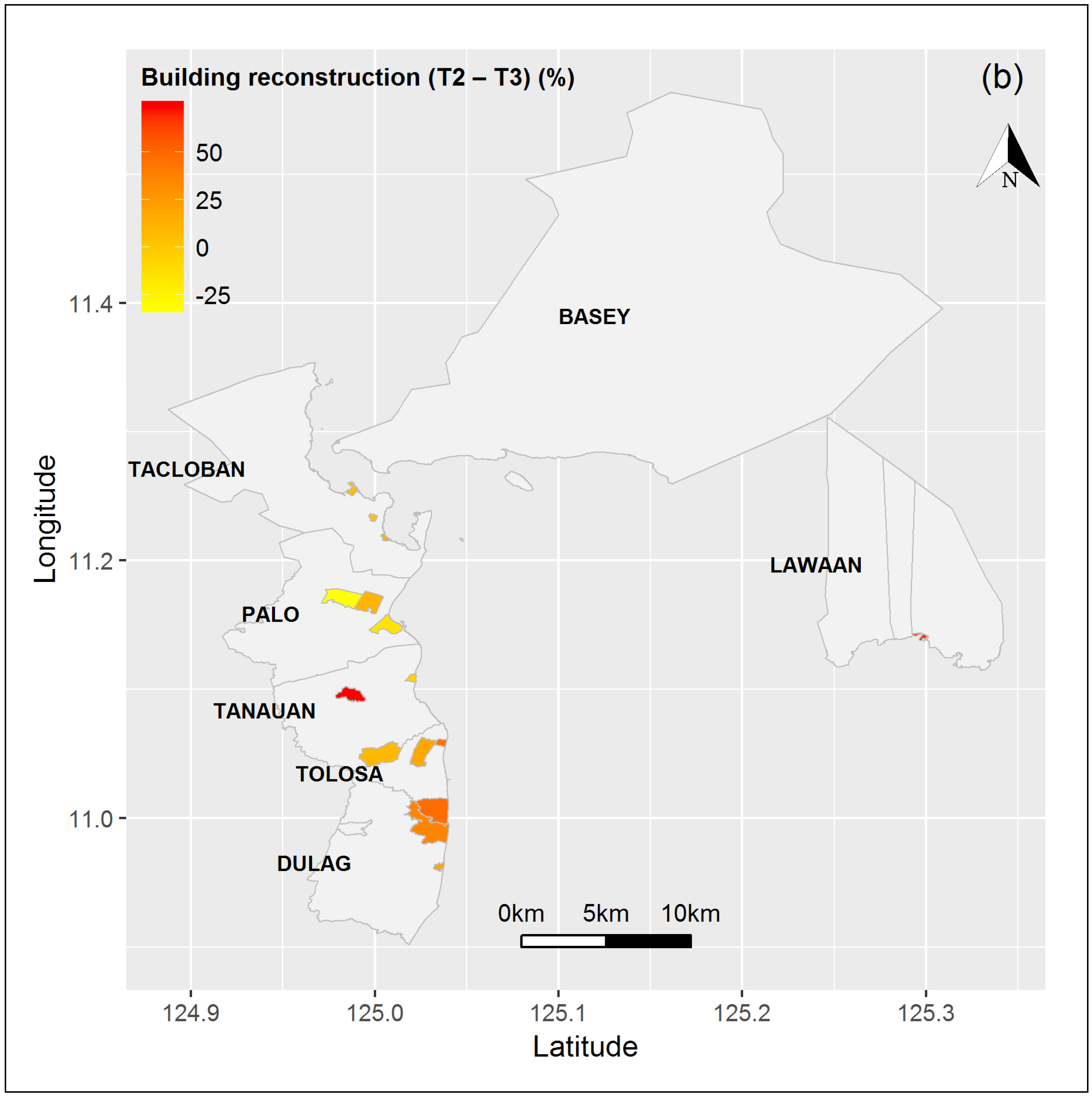Figure 2 shows the seven municipalities that contained the barangays included in this study.

3.4. RS Data Analsyis

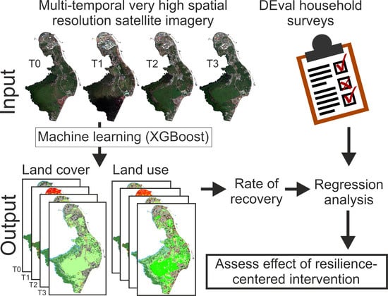
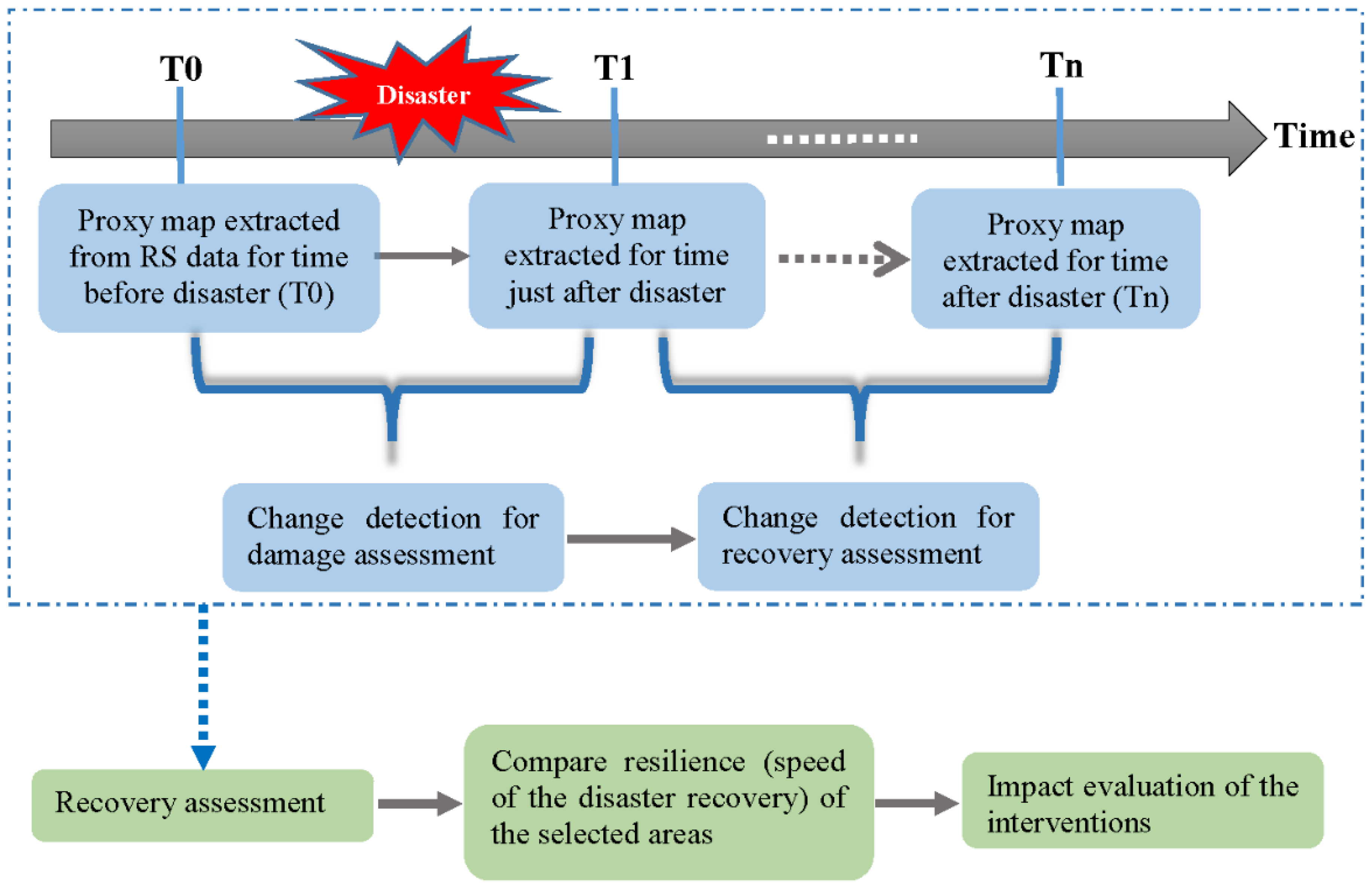
We developed a conceptual framework to assess recovery based on the extraction of image-based proxies. The approach consisted of two main steps: (i) to generate the damage map, and (ii) to generate recovery maps at the required times after the disaster. To do so, suitable proxies needed to be identified and extracted for each of the required time steps (e.g., pre-disaster, event time, and post-disaster). Proxies for separate dimensions, i.e., built-up, social, and economic [19] are needed to cover the entire damage and recovery process comprehensively. The proxies listed for the pre-disaster (T0) and event (T1) times support the damage assessment, and subsequently the damage map was compared with the proxies listed for two post-disaster time epochs approximately 2 and 3 years after Haiyan (T2 and T3, respectively) to assess recovery at each time. The changes in the state of each proxy between two epochs demonstrate the damage to the indicators, and subsequently the degree of recovery.

Table 2. The proxies used for the recovery assessment.

Proxy	Category	Description
Building damage	Built up	Number of damaged/collapsed buildings
Texture	Built up	To extract damaged buildings, roads, and urban areas
Building removal and reconstruction	Built up	To detect recovered buildings
Blow-out debris	Built up	To detect blocked roads and damaged buildings
Reconstruction of bridges and public transport facilities	Built up	Accessibility and transportation facility assessments
Impervious surface	Built up	To extract built-up area and permeability of the surface
Presence of vehicles	Built up/Economic	For transportation condition/accessibility analysis and functioning of roads, and to extract the level of economic activities
Land use (large-scale industry)	Economic	Economic activity types/location and economic focal spaces
Presence of boats	Economic	Fishery industry for livelihood recovery
Arable land	Economic	Agriculture industry for livelihood recovery
Roof color and material	Economic	Industry recovery
Proportion of built-up and vegetated area	Social	Settlement type/location in urban areas
Share of population in irregular clusters	Social	Irregular building clusters link to people with low income/economy (slum area)

shows the selected proxies and their use to evaluate recovery in the selected study area. To assess the full scope of damages we employed proxies that measure the structural damages to buildings, bridges, and transportation facilities, but also textural proxies and evidence of blow-out debris. To assess the recovery process we employ proxies that measure the reconstruction of buildings and impervious surface. Once the proxy-based damage map has been produced, monitoring changes through the built-up proxies indicates the degree of recovery at a given point in time following the disaster. Among the economic proxies, LU information indicates the types of economic activity, while the presence of vehicles and boats provides an indication of the extent and frequency of its use. Arable land is a proxy for the potential for farming. In addition, roof color and material helps to differentiate between types of buildings (e.g., industrial facilities vs. residential housing). We use the share of population residing in informal settlements (i.e., slums) as a proxy for the socio-economic status of the area.

Machine learning methods such as support vector machines (SVM) and random forest (RF) have been widely used in remote sensing data processing, particularly for satellite image processing, due to their efficiency and accurate results. Several researchers also studied their applicability in producing accurate LC and LU maps from remote sensing optical images [20,51,52,53,54]. Recent advances in computer science motivated researchers to use deep learning and convolutional neural network (CNN) approaches as superior classification methods [55]. However, CNN-based models must be trained with a large number of samples to give appropriate results, which also require substantially more computational power and complex models.

Other advanced ML methods have been developed to support challenging image classification tasks at low computational costs, such as logistic model trees, and rotation forest ensembles. The gradient boosting method (GBM) is a supervised classification technique and belongs to regression and classification trees models [56,57]. Tree boosting is an ensemble learning algorithm that is very effective in the classification of even weak trees [58], as has been shown in scene classification [59,60]. However, traditional GBMs require the tuning of a number of parameters and are thus more susceptible to overfitting than other ML algorithms, such as SVM. In 2008, Chen and Guestrin [61] developed the extreme gradient boosting (XGBoost) method, which is the regularized version of GBM and overcomes most of the limitations. Since then XGBoost has been successfully used for different classification problems. Its superiority for LC and LU classification from very high resolution images was also shown in recent studies [58,62].

Both urban and rural LU classes in most cases cannot be distinguished using only spectral information (e.g., slum areas), and require the addition of spatial features (i.e., texture) [63]. Local Binary Patterns (LBP) have been shown to be an effective textural information extraction method [20,64,65]. LBP are based on the gray level co-occurrence matrix, which contains simple textural computations such as mean, variance, homogeneity and entropy. Therefore, in this study the LBP of each image, using a 5 × 5 kernel, were computed and used as input in addition to the image bands in the XGBoost classification. The implementation of the XGBoost classifier was based on the default parameter values, and the calculation of the LBP and XGBoost was performed in Python.

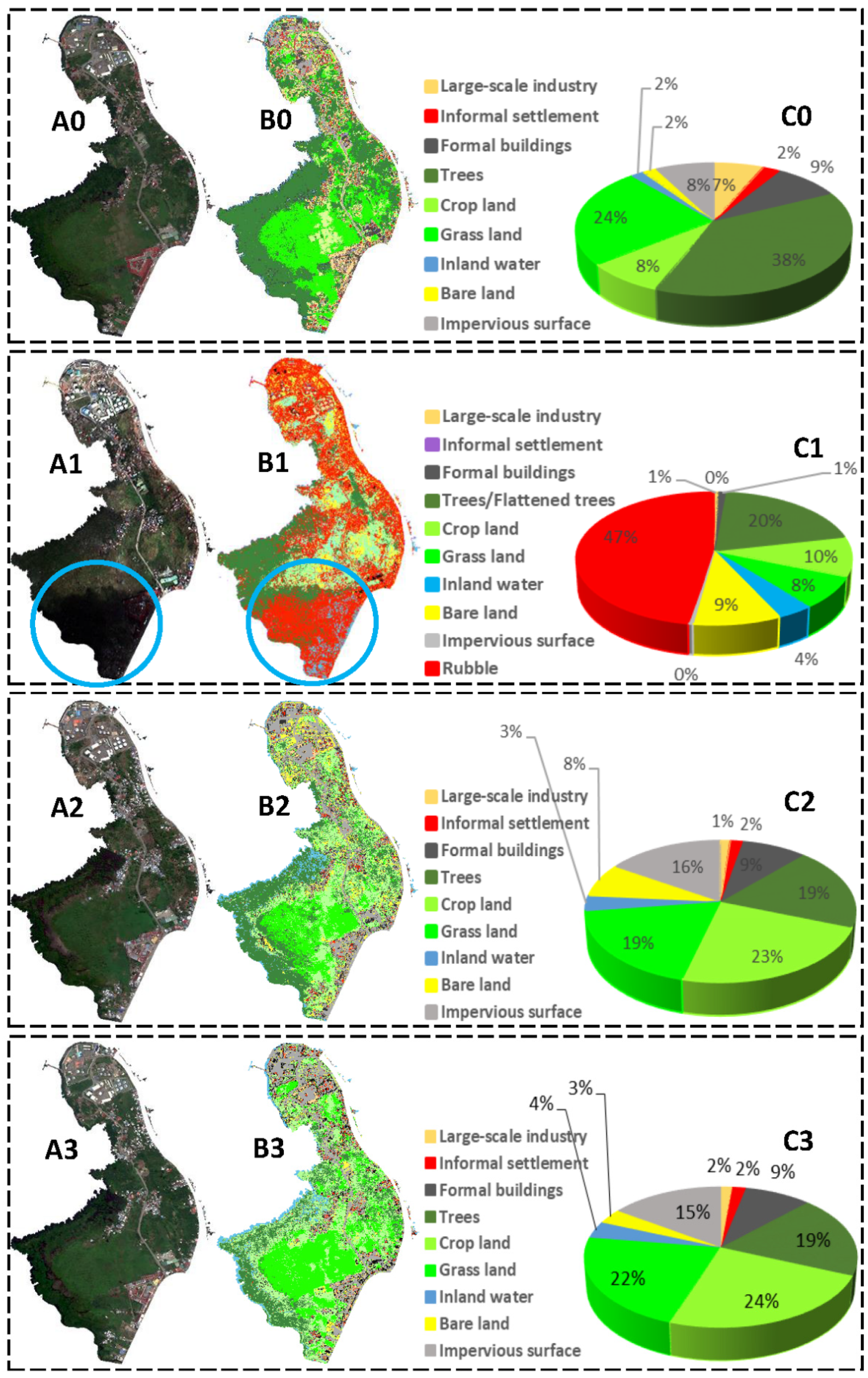
The LC map contains the following classes: building, impervious surface, bare land, inland water, trees/flattened trees, non-tree vegetation, and rubble for the event time images. In addition, the LU maps include large-scale industry, informal settlement (slums), formal buildings, trees/flattened trees, crop land, grass land, inland water, bare land, impervious surface, and rubble for event time images. In the first step of the classification the training areas were selected for each class, separately for the LC and LU classifications. In addition, the accuracy of the results was computed based on standard measurements, overall, user’s, and producer’s accuracy (OA, UA, and PA, respectively) for Barangay 69. Stratified random sampling was used to generate random reference points for the evaluation. Considering the size of the test area, a minimum of 30 sample pixels per class for both the LC and LU classification maps were selected to produce reference data.

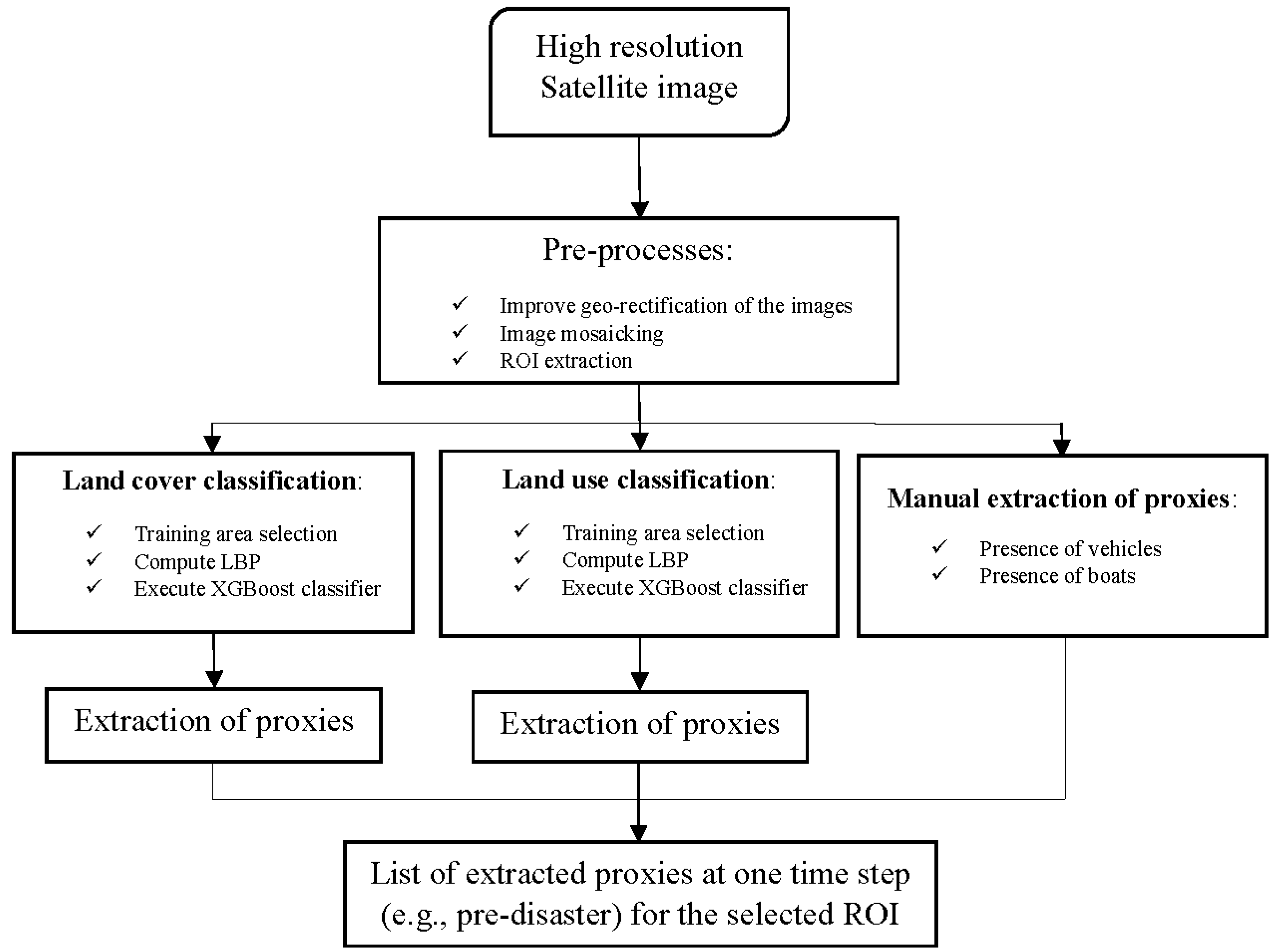
Figure 3 shows the general framework of the implemented steps for the proxy extraction based on LCLU maps. Before starting to select the training areas for the classification, three pre-processes were implemented: (i) improving the geo-referencing of the images; since the final recovery map/proxy extraction was conducted based on a pixel-by-pixel comparison of the maps for each time step, the images required a good matching in terms of geo-referencing. Accordingly, one of the images was selected as a base image, and the geo-referencing of the other images refined using image-to-image registration/rectification, as is commonly done in pixel-based change detection techniques [66]. However, satellite inclination angles vary, and in particular the time-critical post-disaster response phase tends to be dominated by images taken at large off-nadir angles. This leads to errors in the change assessment, in particular for vertical features such as building façades; (ii) image mosaicking to match and merge different satellite images to cover the entire area. The merging operation, and thus the provided merged images, challenge the classification approach and lead to inaccuracies in the LCLU maps, particularly for images collected in different seasons or with large gaps between acquisitions; (iii) region of interest (ROI)/barangay image extraction, which was conducted using ArcGIS based on the barangay boundaries by the United Nation’s Office for Humanitarian Affairs (OCHA) based on information provided by the Philippine Statistical Authority (PSA) [67].

The computed class characteristics were used for the proxy extraction and interpretations. The LCLU classification was implemented on multi-spectral satellite images, while due to their small size compared to other LCLU classes vehicles and boats were extracted using both panchromatic and multispectral images. The boats inside the barangays (on inland water), as well as the boats close to the selected barangays (on open water) were counted. The proxies were extracted based on the LCLU class area sizes and their changes from T0–T3, except for the number of boats and vehicles that were counted manually. For example, the building land cover change from the pre-disaster time (T0) to just after the disaster (T1) shows the change in the overall size of the area covered by buildings in the area and, consequently, the damaged buildings. Furthermore, roof color was calculated based on the extraction of the brightness values of the pixels for the building class using MATLAB.

We implemented the developed approach on the images of the four epochs considered (T0–T3) to extract the selected proxies.

3.5. Statistical Modelling of the Recovery Assessment

Outcome variables. In this study, we focused on building reconstruction and industry recovery as our outcomes of interest. Results from the semi-automated classification of LCLU patterns at the three post-disaster time points (T1–T3) allowed us to compute recovery rates (in %). Positive values indicate an increase in the building stock, while negative values suggest that (possibly damaged) structures were removed.

Survey variables. A selection of relevant variables from the DEval survey was employed in this analysis to investigate the influence of development interventions and various socio-demographic and structural characteristics on recovery rates. We grouped survey variables into donor support, structural characteristics, DRM-related characteristics, and local governance. Donor support was measured with focus on the Germany-funded SIMPLE intervention. A dichotomous variable indicates whether SIMPLE was implemented (1 = yes, 0 = no) in a given barangay, and whether the intervention started early (pre-2009) or late (2009–2012). In addition, we employed a variable measuring whether the barangay had received support from other donors (1 = yes, 0 = no).

Structural characteristics included information on average annual municipal income classified as high (income = 1: ≥500,000 US$) and low (income = 0: <500,000 US$), whether a barangay was located in the city (urban area = 1) or the rural countryside (urban area = 0), and amount of IRA (Internal Revenue Allotment) subsidies (in million $US) that a municipality received during the previous year.

DRM-related characteristics included perceived disaster preparedness, ranked by the barangay captain on a scale from 1 (low) to 10 (high), and whether the barangay had experienced a disaster in the preceding 5 years (1 = yes, 0 = no). In addition, a variable indicated the amount of reconstruction support received by the municipality from government authorities (in million US$), as well as a rating by the barangay captain regarding the number of ongoing DRM-related activities (0 = low, 10 = high).

Finally, the quality of local governance was measured through the political experience level of the barangay captain (1 = more than one completed term as captain, 0 = less than one term as captain), the work experience level of the mayor (years in office), and how corrupt the barangay captain considered the local system to be (0 = low corruption, 10 = high corruption).

Table 3. Summary statistics of the analytical sample.

	Unit	N	Min	Max	Mean	SD
Outcome
Building rec. (T1–T2)	%	14	31.67	1898.9	372.57	505.15
Building rec. (T2–T3)	%	16	−31.45	74.07	22.08	29.73
Industry rec. (T1–T2)	%	13	−30.29	2205.94	397.94	652.92
Industry rec. (T2–T3)	%	13	−45.6	123.83	25	38.9
Donor support
SIMPLE intervention	1|0	18	0	1	0.83	0.38
Late intervention start	1|0	15	0	1	0.4	0.51
Other donor support	1|0	18	0	1	0.83	0.38
Structural characteristics
High income	1|0	18	0	1	0.83	0.38
Urban area	1|0	18	0	1	0.17	0.38
IRA subsidies	US$ (million)	18	0.22	8.86	2.22	3.09
Disaster risk management
Disaster preparedness	scale	18	4	10	7.39	2.33
Disaster experience	1|0	17	0	1	0.76	0.44
Reconstruction support	US$ (million)	13	0.01	1.52	0.33	0.47
DRM activities	scale	18	0	10	5.77	3.1
Local governance
Experienced captain	1|0	18	0	1	0.56	0.51
Experience of mayor	Years	18	1	6	3	2.3
Perceived corruption	Scale	18	0	10	4.83	2.71

Notes: Building rec. = Building reconstruction; Industry rec. = Industry reconstruction; typhoon Haiyan hit the Philippines 7–9 November 2013; T1 = just after disaster, T2 = approx. two years after disaster, T3 = approx. three years after disaster; US$ expressed in current (August 2019) US$.

provides summary statistics for the relevant survey variables.

Statistical approach. Due to the very small sample size the statistical analysis had to be limited to simple bivariate ordinary least squares (OLS) regression models. The primary goal of this analysis was to demonstrate the use of combining RS data with survey data to answer substantively meaningful questions regarding post-disaster recovery processes. Equation (1) formally describes the employed models.

$$y=\alpha +{\beta }_1{x}_1+\mathsf{\epsilon }.$$

(1)

We modeled changes in recovery rates (y) at the barangay level, with α representing the intercept or average recovery rate. The parameter β₁ constitutes the effect of a given predictor variable x₁ (e.g., experience of barangay captain), and $\mathsf{\epsilon }$ constituting the normally distributed error term. To account for the small N, significance tests use robust standard errors. Computations were performed using the R statistical environment [68].

4. Results

4.1. Image-Based Recovery Assessment

The main analysis was conducted based on the proposed methodology for the selected barangays from each municipality. Barangay 69 (0.38 km² in size), located in the North of Tacloban (Figure 2) was selected to visualize the analysis and explain the results in detail for each step. This barangay contains most of the LCLU classes, in addition to some representative challenges/inaccuracies we encountered during the classification and providing the final recovery assessment results.

Figure 4 and Figure 5 show the LC and LU results and their corresponding area coverage ratios for the entire Barangay 69, respectively. The original true color images as well as LCLU maps were provided for each time step to visualize the recovery. However, the selection of the training areas was challenging for some classes, particularly for LU, such as distinguishing the large-scale industry facilities from formal buildings without using auxiliary data.

The developed approach resulted in overall accuracy scores of 85.4%, 76.1%, 83.4%, and 86.0% for the LC classification at T0, T1, T2, and T3 images, respectively, which demonstrated the robustness of the method in classifying the land covers from satellite images (

Table 4. The LC classification accuracies for T0, T1, T2, and T3 time epochs for Barangay 69. User’s and producer’s accuracies and corresponding errors are computed across the study area from the confusion matrices. PA—producer’s accuracy; UA—user’s accuracy; OA—overall accuracy; N.S—number of samples used for the accuracy assessment.

Time/Class		Buildings	Impervious Surface	Bare Land	Water	Trees	Non-Tree Vegetation	Rubble
Pre-disaster (T0)	N.S.	40	40	40	40	40	40	---
	PA%	72.0	89.2	82.9	95.0	97.1	81.8	---
	UA%	90.0	82.5	72.5	95.0	82.5	90.0	---
	OA%	85.4
Just after disaster (T1)	N.S.	40	30	30	30	30	30	44
	PA%	92.5	76.9	80.0	94.7	65.9	79.4	58.7
	UA%	92.5	66.7	66.7	60.0	96.7	90.0	61.1
	OA%	76.1
Post-disaster (T2)	N.S.	30	30	30	30	30	37	---
	PA%	69.2	100	82.8	96.2	72.2	91.7	---
	UA%	90.0	70.0	80.0	83.3	86.7	89.2	---
	OA%	83.4
Post-disaster (T3)	N.S.	30	30	30	30	30	50	---
	PA%	71.1	87.5	81.5	100	85.3	93.5	---
	UA%	90.0	70.0	73.3	100	96.7	86.0	---
	OA%	86.0

). However, the user’s accuracy (UA) values of the impervious surface and water classes were 66.7% and 60.0%, respectively, which shows the relatively high commission error for those classes. In addition, overall accuracies of the LU maps produced by the developed method were 81.8%, 72.1%, 78.7%, and 78.8% for T0, T1, T2, and T3 images, respectively (

Table 5. The LU classification accuracies for T0, T1, T2, and T3 for Barangay 69. User’s and producer’s accuracies and corresponding errors were computed across the study area from the confusion matrices. BareL: bare land; FB: formal built-up area; ImS: impervious surface; LSI: large scale industry; IS: informal settlement; PA—producer’s accuracy; UA—user’s accuracy; OA—overall accuracy; N.S.—number of samples used for the accuracy assessment.

Time/Class		BareL	Crop	FB	Grass	ImS	Water	LSI	IS	Trees	Rubble
Pre-disaster (T0)	N.S.	30	30	35	30	30	30	30	30	40	---
	PA%	78.6	95.7	75.9	90.3	71.0	78.8	87.5	53.5	90.7	---
	UA%	73.3	73.3	73.3	86.7	73.3	86.7	70.0	76.7	97.5	---
	OA%		81.8
Just after disaster (T1)	N.S.	30	30	30	30	30	30	36	30	30	47
	PA%	74.2	100	78.3	60.5	72.4	100	71.1	---	55.8	61.4
	UA%	76.7	53.3	60.0	76.7	70.0	50.0	88.9	---	96.7	67.5
	OA%		72.1
Post-disaster (T2)	N.S.	30	30	32	30	30	30	30	30	31	---
	PA%	87.1	93.8	75.9	64.1	91.3	96.3	70.0	60.6	66.7	---
	UA%	90.0	50.0	73.3	83.3	70.0	86.7	70.0	66.7	75.0	---
	OA%		78.7
Post-disaster (T3)	N.S.	30	30	30	30	30	30	30	30	30	---
	PA%	90.9	100	67.7	80.0	80.0	90.3	61.1	63.6	70.7	---
	UA%	66.7	53.3	70.0	93.3	66.7	93.3	73.3	70.0	72.5	---
	OA%		78.8

). More classes and their similarity in the LU classification, which challenges the classification process, resulted in lower accuracy scores when compared to the LC classification. However, the high producer’s accuracy (PA) values for most of the land use classes, ranging from 70% to 100%, demonstrated the low level of omission errors for those classes in such a challenging case. The developed method produced accurate results in classifying roads (impervious surface) and built up areas, as well as the vegetation classes. However, some inaccuracies resulted in particular from the presence of clouds and their corresponding shadows. For example, the T1 image contained a shadowed area that was mainly covered with low-level vegetation and trees; however, in the LCLU maps the area was classified as debris/rubble (Figure 4 and Figure 5).

As can be seen from Figure 5 most of the buildings recovered, while half of the trees had not yet recovered by T3. The latter was to be expected, given that an estimated 33 million coconut trees were destroyed by Haiyan in the Visayas [69], which take 6–8 years to regrow to maturity. This also explains an observed shift in cultivation of palm trees to other crop types, which leads to a decrease in the number of trees in the area. In addition, young replanted trees are not yet detectable in satellite images, which results in them being misclassified as grass or crop land.

Table 6. The extracted results for the selected proxies for Barangay 69, Tacloban. WV2: WorldView2; GE1: GeoEye1.

#	Measurement	Proxies	Pre-Disaster T0 (2013-03-17_WV2)	Event T1 (2013-11-10_GE1)	Post-Disaster T2 (2016-04-24_GE1)	Post-Disaster T3 (2017-03-18_WV2)
1	Building size (m2)	Structural/building damages, and building removal and reconstruction	29,878	3236 1	25,236	26,852
2	Impervious surface area (m2)	Blow-out debris, and reconstruction of bridges and public transport facilities	15,792	3236	28,482	28,270
3	Counted vehicles	Presence of vehicles	9	1	15	10
4	Large-Scale industry (m2)	Large-Scale industry	12,396	1036	2564	2840
5	Crop land (m2)	Crop land	15,526	18,336	43,848	45,086
6	Tree (m2)	Tree	68,102	------ 2	35,318	34,470
7	Count boats	Presence of boats	13	2	32	22
8	Proportion of blue colored roofs (%)	Building rooftop materials	31	15	78	9
9	Proportion of red colored roofs (%)	Building rooftop materials	18	4	7	10
10	Proportion of white colored roofs (%)	Building rooftop materials	9	2	11	2
11	Proportion of other colored roofs (%)	Building rooftop materials	42	80	4	78
12	Proportion of built-up area (%)	Proportion of built-up area	24	2	28	29
13	Proportion of vegetated area (%)	Proportion of vegetated area	72	41	61	64
14	Informal settlement size (m2)	Proportion of irregular clusters	4284	0	3138	3484
15	Arable land (m2)	Availability of land for farming	3744	16,740	13,998	6106

¹ The extremely low post-event (T1) building size value suggests that more than 90% of all buildings in this barangay were destroyed; however, it instead implies that some degree of damage were detected on nearly all buildings. ² Most of the trees in Barangay 69 were coconut palm trees that were destroyed during Haiyan. However, some trees were left standing, but those cannot be distinguished from flattened trees in the satellite imagery used, hence here we assumed that in T1 all trees were destroyed.

shows the final extracted proxies. Almost 80% of the buildings in Barangay 69 had been reconstructed/had recovered by March 2017. However, the area covered by both industrial buildings and informal settlements (slums) decreased. The latter were marked by clusters with highly irregular patterns, and their share decreased, which illustrates a positive recovery aspect after the disaster.

4.2. Statistical Analysis Results

Combining results from the semi-automated LCLU classification with survey data we provide an example of how RS data and survey information can be meaningfully combined in evaluation work.

Table 7. Results from OLS regression models predicting building reconstruction and industry recovery.

	Building Rec. (T1–T2)		Building Rec. (T2–T3)		Industry Rec. (T1–T2)		Industry Rec. (T2–T3)
	b	sig	b	sig	b	sig	b	sig
Donor support
SIMPLE intervention	−50.51		−44.52	***	264.84		−107.06	***
Late intervention start	491.63		−0.23		737.15	+	−19.47
Other donor support	−1069.6	*	19.05	+	−386.39		−6.5
Structural characteristics
High income	332.69	+	−17.63		464.79	+	12.68
Urban area	936.72	*	−16.47		397.47		6.27
IRA subsidies	112.85	*	−2.86	*	54.26		0.42
Disaster risk management
Disaster preparedness	22.22		−2.69		−93.43		6.93
Disaster experience	−665.88		−29.28		−357.7		−75.39	*
Reconstruction support	−57.11		−50.02	***	−58.45		−14.52
DRM activities	−34.87		0.5		−73.36		−6.32
Local governance
Experienced captain	−38.14		−8.7		−439.61		15.56
Experience of mayor	−87.29	+	−3.41		−125.83	+	−0.63
Perceived corruption	−86.55	*	6.21	*	−70.67		2.17

Notes: + p < 0.10; * p < 0.05; ** p < 0.01; *** p < 0.001; typhoon Haiyan hit the Philippines 7–9 November 2013; T1 = just after disaster, T2 = approx. two years after disaster, T3 = approx. three years after the disaster; T1–T2 = early recovery phase; T2–T3 = late recovery phase; separate OLS regression models were estimated for each predictor; significance tests based on robust standard errors.

shows the results from the OLS regression model predicting short-term and long-term building reconstruction and industry recovery.

Donor support. A primary question we were interested in was how the German-funded SIMPLE intervention related to post-Haiyan recovery rates. Note that our analytical design (purposeful sample selection) did not permit rigorous causal attribution (see Discussion). We found no significant relationship between the SIMPLE intervention and the early recovery phase (T1–T2). However, the relationship was significant (p < 0.001) and negative during the late recovery phase (T2–T3). For example, the building recovery rate was about 45% lower in barangays that received the SIMPLE intervention compared to those that did not. Figure 6 shows building recovery rates and the intervention per barangay, which allows for a visual appraisal of the observed correlation. Similar to the SIMPLE intervention, the only significant effect of other donor support was negative and emerged for building reconstruction in the early recovery phase (b = −1069.6, p < 0.05).

Structural characteristics. For structural characteristics, significant relationships emerged mainly for building reconstruction, while industry recovery was comparatively unaffected. We observed higher growth rates in urban vs. rural areas (b = 936.72, p < 0.05). Barangays that received IRA subsidies showed higher reconstruction rates (b = 112.85, p < 0.05) during the early phase, but negative reconstruction rates (b = −2.86, p < 0.05) during the late phase.

Disaster risk management. Those barangays that had previously experienced a natural disaster showed slower industry recovery rates (b = −75.39, p < 0.05) than those without such experiences. Moreover, our analysis revealed that reconstruction support was significantly related to a lower building reconstruction rate in the later phase (b = −50.02, p < 0.001).

Local governance. Good governance may facilitate the recovery process through administrative support, procurement of financial resources, and implementation of guidelines and standards. Yet, in our analysis we found little relationship of the level of experience of the local leaders (e.g., mayor, barangay captain) with recovery speed. However, the perceived level of corruption influenced the speed of building reconstruction. Barangays with high levels of corruption experienced significantly slower (b = −86.55, p < 0.05) building reconstruction rates in the early phase, but slightly higher rates (b = 6.21, p < 0.05) in the later phase.

5. Discussion

The underlying assumption in this work was that communities that received DRR-related interventions such as assistance with comprehensive land-use planning would perform better in the aftermath of a major disaster than those without, and we considered post-disaster recovery to be a proxy of resilience. The analysis of high spatial resolution satellite images for 18 barangays provided a detailed picture of LCLU changes caused by typhoon Haiyan and the recovery efforts during the subsequent 3 years. The developed conceptual framework based on a range of proxy indicators primarily extracted through ML allowed the quantification of reconstruction in both formal and informal settlements, as well as of industrial facilities, but also changes in agricultural LU. As such we demonstrated the utility of RS to detect and characterize recovery, similar to [20], who did this for the city of Tacloban only. Nevertheless, the inherently descriptive nature and resulting limitation of RS data became apparent, in that the reasons for the spatially and temporally highly variable recovery performance observed could not be determined. We made use of survey information derived from 3000 household interviews conducted by DEval. Those are suitable to generate very detailed insights into DRR-related perspectives, motivations, and drivers of the affected population. However, their acquisition required a considerable effort and planning horizon. In addition, socio-economic data are frequently limited when it comes to assessing physical characteristics such as infrastructural changes. While the survey data are able to reveal changes in DRR-related perceptions and motivations of humans, they are not suitable to estimate actual recovery processes such as building reconstruction or industry recovery. Combining the RS-based measures of post-disaster recovery with detailed survey information allows embedding the physical recovery process within the socioeconomic context.

However, while the image analysis does provide detailed information about LC and LU changes directly linked to recovery, the observed recovery performance could not always be unambiguously explained by the socioeconomic data. For example, contrary to expectation we observed slower recovery rates in barangays that had received the SIMPLE intervention or other donor support, but also for those communities with prior disaster experience. This may be the consequence of more rigorous planning efforts and stricter building policies. As such slower recovery may signal higher quality of the newly established building stock and could indicate higher resilience, including to future events. Nevertheless, this does not agree with the generally accepted notion of resilient communities showing faster recovery [19,20]. The image analysis did show an overall rapid and positive recovery, with building stock getting reconstructed quickly (although more rapidly in urban than in rural communities), with the proportion of informal settlements declining, and some adaptation in the agricultural sector, such as vulnerable coconut palms getting replaced by other crops. The statistical analysis also showed that some of the poorer barangays rebuilt quickly, as they received additional IRA funding, though the effect was ephemeral and may thus signal the lack of more comprehensive recovery planning, and sustained means to fund its implementation.

The DEval evaluation gave a detailed picture of the impacts of a comprehensive land-use planning intervention. It clearly showed the relevance of the intervention, but evidence of effectiveness, impact, and sustainability was mixed [14]. For example, SIMPLE municipalities showed better LU planning quality and comprehensiveness. At the same time, there was little evidence for stronger and wider stakeholder participation, or of the enhanced LU planning the intervention aimed at, especially at household level. Interventions had a positive effect on disaster awareness and proactive management strategies, but the assessment also showed considerable mistrust in local government. In our analysis in particular perceived corruption correlated negatively with recovery speed.

The RS analysis is subject to additional limitations. The quantification of recovery hinges on an accurate initial damage assessment. However, RS-based damage detection continues to pose challenges, even if very high resolution images are used [17,70], and in particular when volunteers carry out the immediate post-disaster damage mapping [71,72]. In particular in the main affected coastal areas of Tacloban and Basey the blanket coverage with washed-up or wind-blown rubble and debris led to strong damage overestimation in published maps [73]. In particular the structural rubble of buildings that were partly or several damaged effectively blended in with the surrounding debris (Figure 7), severely challenging both visual and automated damage detection.

An analysis of the damage map created during a Humanitarian OpenStreetMap campaign showed an overestimation of destroyed buildings in Tacloban by some 92% [74], and also the damage and resulting recovery maps in [20,75] show this overestimation to some extent. It is likely that some of the barangays that in this study show building reconstruction rates of >1000% within about 3 years also suffered less actual building damage. In addition some of the proxies used in the analysis, in particular LU classes such as crop or tree types, but also related to building and settlement type, suffer from uncertainties. Using high-resolution unmanned aerial vehicle (UAV)/drone images (e.g., Figure 7a) instead of satellite data can reduce the debris problem and lead to more accurate damage detection results. However, the aim of this work was to test the suitability of multi-temporal satellite images that potentially allows a synoptic recovery assessment at any desired time interval, while both the availability and spatial coverage of UAV data are typically limited. In addition, recent work on structural damage mapping with UAV has also demonstrated the limits of those data [76], even when advanced deep learning methods are used [77].

While it would also have been ideal to process images covering all 100 DEval municipalities, this would have been prohibitive in terms of image and processing costs. The narrow coastal strip from Tacloban to Dulag alone covers an area of approximately 400 km². A single high resolution multispectral Pléiades images for this area would cost in excess of 5000 US$, while an 8-band WorldView-3 image would cost about 7500 US$, and a simple recovery assessment requires three time steps as a minimum (T0, T1, and T2). For the image analysis part of this work we made use of image data costing approximately 45,000 US$, part of which was donated by the Digital Globe Foundation. In particular immediate post-event images are also often acquired at large off-nadir angles, resulting in additional challenges for detailed recovery assessment [75]. The recent recovery study that focused on Tacloban [20] showed that a detailed LU classification that is needed for comprehensive urban recovery assessment requires very high spatial resolution imagery. However, it also showed that lower resolution data suffice for a LC assessment in urban areas, and are also suitable to support the quantification of recovery in rural areas, where the size of relevant objects tends to be larger. This means that a more optimized use of images can be achieved, i.e., very high spatial resolution imagery is not always needed.

6. Conclusions

The purpose of this study was to evaluate the usefulness of combining RS with field-based survey data in the assessment of resilience-centered interventions. We initially hypothesized that image data could add critical additional information to the questionnaire-based evaluation, and might allow an extrapolation to areas with fewer or no interviews. However, it became clear quickly that matching a RS analysis to the spatial extent of the DEval study (100 municipalities spread over two regions) was prohibitive. In addition to cost, many of the more outlying communities are not adequately covered in high resolution data catalogues. Conversely, the statistical analysis in this study showed that it was actually the survey information that added value to the interpretation of the LCLU classification results. Similar to other recent work e.g., [e.g., 20] the limitations of RS to explain spatially and temporally variable recovery also became clear here, and the field-based information proved valuable.

Regarding the utility of RS data to support intervention evaluations, current limitations are clear. Vast amounts of detailed image data are necessary, resulting also in high processing cost. However, the efficiency and sophistication of damage- and recovery-focused processing has also been increasing, in particular through advances in deep learning/CNN [75,78], where a trend towards automatically handling large datasets as training samples is evident. However, even when sophisticated image processing methods were used in our study also showed that remote sensing-based recovery assessment, which requires LCLU-based change analysis over multi-temporal data, significantly depended on the accuracy of the image classification results. For example, the overestimation of the building class in the pre-disaster image might lead to the extraction of negative recovery for buildings, which might not be correct.

One of the critical aspects related to resilience is climate change adaptation. This can include physical measures such as dikes or dams, but increasingly nature-based solutions are sought [79,80], and remote sensing has shown its utility in monitoring many relevant indicators [81]. In coastal communities such as the ones studied in this work, which are subject to rising sea levels, salt water intrusion, and regular tropical storms, image data have tremendous potential in detecting and quantifying adaptive measures, such as vulnerable crops (e.g., coconut palms) getting replaced by more resilient solutions, or protective mangrove corridors getting reinstated. Evidence of such actions can be a valuable addition to household surveys. For rural areas and crop monitoring it may be possible to work with freely available data, such as 3–5 m resolution images from Planet. However, more work is needed in this area.

Due to the high costs for image data and high demand on human resources (coding and manual data processing), we were unable to compute LC and LU for the full sample of municipalities (N = 100) for which socioeconomic survey data were available via the DEval impact evaluation. Since we purposefully selected seven municipalities (13–18 barangays), our analysis did not permit a rigorous attribution of causal impacts and the results of the statistical analysis should be interpreted with caution given the small sample size. Nevertheless, the purpose of this work was to provide a proof of concept of meaningfully integrating socio-economic survey data with RS data to combine the strength of both in an attempt to harness synergies. Building on this work, future research may employ a geospatial impact evaluation designs (GIE) [15], and use matching techniques to obtain a sufficiently large sample of control and intervention barangays. Following the computation of RS-based recovery measures for all units, statistical methods such as the difference-in-difference approach (see Section 2) would then permit to connect program effects with recovery processes causally. With a sufficiently large sample the full potential of combining survey information with RS data could then be realized beyond what was possible here.

References

1. UNISDR. Global Assessment Report on Disaster Risk Reduction; UNISDR: Geneva, Switzerland, 2015; p. 316. [Google Scholar]
2. Mochizuki, J.; Naqvi, A. Reflecting disaster risk in development indicators. Sustainability 2019, 11, 14. [Google Scholar] [CrossRef]
3. The World Bank. Results Brief—Climate Insurance. Available online: https://www.worldbank.org/en/results/2017/12/01/climate-insurance (accessed on 9 October 2019).
4. Kharin, V.V.; Zwiers, F.W.; Zhang, X.B.; Hegerl, G.C. Changes in temperature and precipitation extremes in the IPCC ensemble of global coupled model simulations. J. Clim. 2007, 20, 1419–1444. [Google Scholar] [CrossRef]
5. Bengtsson, L.; Hodges, K.I.; Roeckner, E. Storm tracks and climate change. J. Clim. 2006, 19, 3518–3543. [Google Scholar] [CrossRef]
6. Hsiang, S.; Kopp, R.; Jina, A.; Rising, J.; Delgado, M.; Mohan, S.; Rasmussen, D.J.; Muir-Wood, R.; Wilson, P.; Oppenheimer, M.; et al. Estimating economic damage from climate change in the United States. Science 2017, 356, 1362–1368. [Google Scholar] [CrossRef]
7. Tol, R.S.J. The economic impacts of climate change. Rev. Env. Econ. Policy 2018, 12, 4–25. [Google Scholar] [CrossRef]
8. UNEP. The Adaptation Gap Report 2017; United Nations Environment Programme (UNEP): Nairobi, Kenya, 2017; p. 85. [Google Scholar]
9. Gertler, P.J.; Martinez, S.; Premand, P.; Rawlings, L.; Vermeersch, C. Impact Evaluation in Practice, 2nd ed.; World Bank Group: Washington, DC, USA, 2016; p. 335. [Google Scholar]
10. MPC. Integrated Public Use Microdata Series, International: Version 7.1 [Dataset]; Minnesota Population Center: Minneapolis, MN, USA, 2018. [Google Scholar]
11. ICF. Demographic and Health Surveys; ICF: Rockville, MD, USA, 2019. [Google Scholar]
12. Luke, D.A. Multilevel Modeling; Sage: Thousand Oaks, CA, USA, 2004; Volume 143. [Google Scholar]
13. Lech, M.; Harten, S.; Uitto, J.I.; Batra, G.; Anand, A. Improving international development evaluation through geospatial data and analysis. Int. J. Geospat. Environ. Res. 2018, 5, 3. [Google Scholar]
14. Leppert, G.; Hohfeld, L.; Lech, M.; Wencker, T. Impact, Diffusion and Scaling-Up of a Comprehensive Land-Use Planning Approach in the Philippines. From Development Cooperation to National Policies; German Institute for Development Evaluation (DEval): Bonn, Germany, 2018. [Google Scholar]
15. Ben Yishay, A.; Runfola, D.; Tricher, R.; Dolan, C.; Goodman, S.; Parks, B.; Tanner, J.; Heuser, S.; Batra, G.; Anand, A. A Primer on Geospatial Impact Evaluation Methods, Tools, and Applications; AidData: Williamsburg, VA, USA, 2017. [Google Scholar]
16. Pech, L. Development of an urban area of limited statehood observed from above: The case of Goma, Democratic Republic of the Congo. In Measuring Statehood on a Sub-National Level: A Dialogue among Methods; Collaborative Research Center (SFB) 700: Berlin, Germany, 2017; pp. 27–34. [Google Scholar]
17. Kerle, N. Disasters: Risk assessment, management, and post—Disaster studies using remote sensing. In Remote Sensing of Water Resources, Disasters, and Urban Studies (Remote Sensing Handbook, 3); Thenkabail, P.S., Ed.; CRC Press: Boca Raton, FL, USA, 2015; pp. 455–481. [Google Scholar]
18. Ebert, A.; Kerle, N.; Stein, A. Urban social vulnerability assessment with physical proxies and spatial metrics derived from air- and spaceborne imagery and GIS data. Nat. Hazards 2009, 48, 275–294. [Google Scholar] [CrossRef]
19. Ghaffarian, S.; Kerle, N.; Filatova, T. Remote sensing-based proxies for urban disaster risk management and resilience: A review. Remote Sens. 2018, 10, 1760. [Google Scholar] [CrossRef]
20. Sheykhmousa, M.; Kerle, N.; Kuffer, M.; Ghaffarian, S. Post-disaster recovery assessment with machine learning-derived land cover and land use information. Remote Sens. 2019, 11, 1174. [Google Scholar] [CrossRef]
21. Dupas, P. Do teenagers respond to HIV risk information? Evidence from a field experiment in Kenya. Am. Econ. J. Appl. Econ. 2011, 3, 1–34. [Google Scholar] [CrossRef]
22. Duflo, E.; Dupas, P.; Kremer, M. Peer effects, teacher incentives, and the impact of tracking: Evidence from a randomized evaluation in Kenya. Am. Econ. Rev. 2011, 101, 1739–1774. [Google Scholar] [CrossRef]
23. De Janvry, A.; Finan, F.; Sadoulet, E. Local electoral incentives and decentralized program performance. Rev. Econ. Stat. 2012, 94, 672–685. [Google Scholar] [CrossRef]
24. Mu, R.; Van de Walle, D. Rural roads and local market development in Vietnam. J. Dev. Stud. 2011, 47, 709–734. [Google Scholar] [CrossRef]
25. McKenzie, D.; Puerto, S.; Odhiambo, F. Unpacking the Determinants of Entrepreneurship Development and Economic Empowerment for Women in Kenya; International Initiative for Impact Evaluation (3ie): New Delhi, India, 2019. [Google Scholar]
26. Alix-Garcia, J.; McIntosh, C.; Sims, K.R.E.; Welch, J.R. The ecological footprint of poverty alleviation: Evidence from Mexico’s Oportunidades program. Rev. Econ. Stat. 2013, 95, 417–435. [Google Scholar] [CrossRef]
27. Fort, R. The homogenization effect of land titling on investment incentives: Evidence from Peru. NJAS Wagening. J. Life Sci. 2008, 55, 325–343. [Google Scholar] [CrossRef]
28. Bensch, G.; Peters, J. Alleviating deforestation pressures? Impacts of improved stove dissemination on charcoal consumption in urban Senegal. Land Econ. 2013, 89, 676–698. [Google Scholar] [CrossRef]
29. Doswald, N.; Sanchez Torrente, L.; Reumann, A.; Moull, K.; Rocio Pérez, J.; Köngeter, A.; Fernandéz de Velasco, G.; Leppert, G.; Puri, J. Evidence Gap Map of Climate Change Adaptation Interventions in Low and Middle Income Countries; Green Climate Fund & DEval: Songdo, Korea; Bonn, Germany, 2019. [Google Scholar]
30. Nawrotzki, R. The Geodata Decision Tree: Using Geodata for Evaluations; Deutsches Evaluierungsinstitut der Entwicklungszusammenarbeit: Bonn, Germany, 2019. [Google Scholar]
31. Coppola, D.P. Chapter 1—The Management of Disasters. In Introduction to International Disaster Management, 3rd ed.; Coppola, D.P., Ed.; Butterworth-Heinemann: Boston, MA, USA, 2015; pp. 1–39. [Google Scholar] [CrossRef]
32. Arciniegas, G.; Bijker, W.; Kerle, N.; Tolpekin, V.A. Coherence- and amplitude-based analysis of seismogenic damage in Bam, Iran, using Envisat ASAR data. IEEE Trans. Geosci. Remote Sens. 2007, 45, 1571–1581. [Google Scholar] [CrossRef]
33. Saito, K.; Spence, R.J.S.; Going, C.; Markus, M. Using high-resolution satellite images for post-earthquake building damage assessment: A study following the 26 January 2001 Gujarat earthquake. Earthq. Spectra 2004, 20, 145–169. [Google Scholar] [CrossRef]
34. Berke, P.R.; Kartez, J.; Wenger, D. Recovery after disaster—Achieving sustainable development, mitigation and equity. Disasters 1993, 17, 93–109. [Google Scholar] [CrossRef]
35. Mueller, M.; Segl, K.; Heiden, U.; Kaufmann, H. Potential of high-resolution satellite data in the context of vulnerability of buildings. Nat. Hazards 2006, 38, 247–258. [Google Scholar] [CrossRef]
36. MCDEM. Focus on Recovery: A Holistic Framework for Recovery in New Zealand; Ministry of Civil Defence & Emergency Management: Wellington, New Zealand, 2005; p. 29.
37. Morrow, B.H. Identifying and mapping community vulnerability. Disasters 1999, 23, 1–18. [Google Scholar] [CrossRef] [PubMed]
38. Flax, L.K.; Jackson, R.W.; Stein, D.N. Community vulnerability assessment tool methodology. Nat. Hazards Rev. 2002, 3, 163–176. [Google Scholar] [CrossRef]
39. Burton, C.G. The Development of Metrics for Community Resilience to Natural Disasters. Ph.D. Thesis, University of South Carolina, Columbia, SC, USA, 2012. [Google Scholar]
40. Bradshow, S. Socio-Economic Impacts of Natural Disaster: A Gender Analysis; Series Manuales 32; Nation Economic Commission for Latin America (ECLA): Santiago, Chile, 2004. [Google Scholar]
41. Bevington, J.; Pyatt, S.; Hill, A.; Honey, M.; Adams, B.; Davidson, R.; Brink, S.; Chang, S.; Panjwani, D.; Mills, R.; et al. Uncovering Community Disruption Using Remote Sensing: An Assessment of Early Recovery in Post-Earthquake Haiti; University of Delaware, Disaster Research Center: Newark, DE, USA, 2010; p. 22. [Google Scholar]
42. Rubin, C.B.; Saperstein, M.D.; Barbee, D.G. Community Recovery from a Major Natural Disaster; Monograph 41; Institute of Behavioral Science, University of Colorado: Boulder, CO, USA, 1985. [Google Scholar]
43. Reif, M.K.; Macon, C.L.; Wozencraft, J.M. Post-Katrina land cover, elevation, and volume change assessment along the South shore of Lake Pontchartrain, Louisiana, USA. J. Coast. Res. 2011, 62, 30–39. [Google Scholar] [CrossRef]
44. Rau, J.Y.; Chen, L.C.; Liu, J.K.; Wu, T.H. Dynamics monitoring and disaster assessment for watershed management using time-series satellite images. IEEE Trans. Geosci. Remote Sens. 2007, 45, 1641–1649. [Google Scholar] [CrossRef]
45. Daniell, J.; Mühr, B.; Girard, T.; Dittrich, A.; Fohringer, J.; Lucas, C.; Kunz-Plapp, T. Super Typhoon Haiyan/Yolanda—Report No. 2; Center for Disaster Management and Risk Reduction Technology (CEDIM), Karlsruhe Institute of Technology: Karlsruhe, Germany, 2013; p. 25. [Google Scholar]
46. Lagmay, A.M.F.; Agaton, R.P.; Bahala, M.A.C.; Briones, J.; Cabacaba, K.M.C.; Caro, C.V.C.; Dasallas, L.L.; Gonzalo, L.A.L.; Ladiero, C.N.; Lapidez, J.P.; et al. Devastating storm surges of Typhoon Haiyan. Int. J. Disaster Risk Reduct. 2015, 11, 1–12. [Google Scholar] [CrossRef]
47. Takagi, H.; Esteban, M. Statistics of tropical cyclone landfalls in the Philippines: Unusual characteristics of 2013 Typhoon Haiyan. Nat. Hazards 2016, 80, 211–222. [Google Scholar] [CrossRef]
48. Kure, S.; Jibiki, Y.; Quimpo, M.; Manalo, U.N.; Ono, Y.; Mano, A. Evaluation of the characteristics of human loss and building damage and reasons for the magnification of damage due to Typhoon Haiyan. Coast. Eng. J. 2016, 58, 27. [Google Scholar] [CrossRef]
49. Boschetti, M.; Nelson, A.; Nutini, F.; Manfron, G.; Busetto, L.; Barbieri, M.; Laborte, A.; Raviz, J.; Holecz, F.; Mabalay, M.R.O.; et al. Rapid assessment of crop status: An application of MODIS and SAR Data to rice areas in Leyte, Philippines affected by Typhoon Haiyan. Remote Sens. 2015, 7, 6535–6557. [Google Scholar] [CrossRef]
50. Garcia Schustereder, M.; Hohfeld, L.; Lech, M.; Leppert, G. Donor-Assisted Land-Use Planning in the Philippines: Insights from a Multi-Level Survey; Deutsches Evaluierungsinstitut der Entwicklungszusammenarbeit (DEval): Bonn, Germany, 2016; p. 84. [Google Scholar]
51. Nery, T.; Sadler, R.; Solis-Aulestia, M.; White, B.; Polyakov, M.; Chalak, M. Comparing supervised algorithms in land use and land cover classification of a Landsat time-series. In 2016 IEEE International Geoscience and Remote Sensing Symposium; IEEE: New York, NY, USA, 2016; pp. 5165–5168. [Google Scholar] [CrossRef]
52. Maxwell, A.E.; Warner, T.A.; Fang, F. Implementation of machine-learning classification in remote sensing: An applied review. Int. J. Remote Sens. 2018, 39, 2784–2817. [Google Scholar] [CrossRef]
53. Ma, L.; Li, M.C.; Ma, X.X.; Cheng, L.; Du, P.J.; Liu, Y.X. A review of supervised object-based land-cover image classification. ISPRS J. Photogramm. Remote Sens. 2017, 130, 277–293. [Google Scholar] [CrossRef]
54. Georganos, S.; Grippa, T.; Vanhuysse, S.; Lennert, M.; Shimoni, M.; Kalogirou, S.; Wolff, E. Less is more: Optimizing classification performance through feature selection in a very-high-resolution remote sensing object-based urban application. GISci. Remote Sens. 2018, 55, IV. [Google Scholar] [CrossRef]
55. Yang, C.; Rottensteiner, F.; Heipke, C. Classification of land cover and land use based on convolutional neural networks. ISPRS Ann. Photogramm. Remote Sens. Spat. Inf. Sci. 2018, IV-3, 251–258. [Google Scholar] [CrossRef]
56. Friedman, J.H. Greedy function approximation: A gradient boosting machine. Ann. Stat. 2001, 29, 1189–1232. [Google Scholar] [CrossRef]
57. Zhu, Y.; Newsam, S. Land Use Classification Using Convolutional Neural Networks Applied to Ground-Level Images; Assoc Computing Machinery: New York, NY, USA, 2015. [Google Scholar] [CrossRef]
58. Ren, X.D.; Guo, H.N.; Li, S.H.; Wang, S.L.; Li, J.H. A novel image classification method with CNN-XGBoost model. In Digital Forensics and Watermarking; Kraetzer, C., Shi, Y.Q., Dittmann, J., Kim, H.J., Eds.; Springer International Publishing AG: Cham, Switzerland, 2017; Volume 10431, pp. 378–390. [Google Scholar]
59. Zhang, F.; Du, B.; Zhang, L.P. Scene classification via a gradient boosting random convolutional network framework. IEEE Trans. Geosci. Remote Sens. 2016, 54, 1793–1802. [Google Scholar] [CrossRef]
60. Chan, J.C.W.; Paelinckx, D. Evaluation of Random Forest and Adaboost tree-based ensemble classification and spectral band selection for ecotope mapping using airborne hyperspectral imagery. Remote Sens. Environ. 2008, 112, 2999–3011. [Google Scholar] [CrossRef]
61. Chen, T.Q.; Guestrin, C. XGBoost: A Scalable Tree Boosting System; Assoc Computing Machinery: New York, NY, USA, 2016; pp. 785–794. [Google Scholar] [CrossRef]
62. Georganos, S.; Grippa, T.; Vanhuysse, S.; Lennert, M.; Shimoni, M.; Wolff, E. Very high resolution object-based land use-land cover urban classification using extreme gradient boosting. IEEE Geosci. Remote Sens. Lett. 2018, 15, 607–611. [Google Scholar] [CrossRef]
63. Chen, C.; Zhang, B.C.; Su, H.J.; Li, W.; Wang, L. Land-use scene classification using multi-scale completed local binary patterns. Signal. Image Video Process. 2016, 10, 745–752. [Google Scholar] [CrossRef]
64. Mboga, N.; Persello, C.; Bergado, J.R.; Stein, A. Detection of informal settlements from VHR images using convolutional neural networks. Remote Sens. 2017, 9, 18. [Google Scholar] [CrossRef]
65. Kuffer, M.; Pfeffer, K.; Sliuzas, R. Slums from space—15 years of slum mapping using remote sensing. Remote Sens. 2016, 8, 29. [Google Scholar] [CrossRef]
66. Singh, A. Digital change detection techniques using remotely-sensed data. Int. J. Remote Sens. 1989, 10, 989–1003. [Google Scholar] [CrossRef]
67. The Humanitarian Data Exchange. Available online: https://data.humdata.org/dataset/philippines-administrative-levels-0-to-3 (accessed on 11 September 2019).
68. R Core Team. R: A Language and Environment for Statistical Computing; R Foundation for Statistical Computing: Vienna, Austria, 2019. [Google Scholar]
69. Acda, M.N. Fuel pellets from downed coconut (Cocos nucifera) in super typhoon Haiyan. Biomass Bioenerg. 2015, 83, 539–542. [Google Scholar] [CrossRef]
70. Kerle, N. Satellite-based damage mapping following the 2006 Indonesia earthquake—How accurate was it? Int. J. Appl. Earth Obs. Geoinf. 2010, 12, 466–476. [Google Scholar] [CrossRef]
71. Kerle, N. Disaster mapping by citizens is limited. Nature 2015, 517, 438. [Google Scholar] [CrossRef] [PubMed]
72. Kerle, N.; Hoffman, R.R. Collaborative damage mapping for emergency response: The role of Cognitive Systems Engineering. Nat. Hazards Earth Syst. Sci. 2013, 13, 97–113. [Google Scholar] [CrossRef]
73. Ghaffarian, S.; Kerle, N. Towards post-disaster debris identification for precise damage and recovery assessments from UAV and satellite images. Int. Arch. Photogramm. Remote Sens. Spat. Inf. Sci. 2019, XLII-2/W13, 297–302. [Google Scholar] [CrossRef]
74. Westrope, C.; Banick, R.; Levine, M. Groundtruthing OpenStreetMap building damage assessment. In Humanitarian Technology: Science, Systems and Global Impact 2014; Vidan, A., Shoag, D., Eds.; Elsevier Science Bv: Amsterdam, The Netherlands, 2014; Volume 78, pp. 29–39. [Google Scholar]
75. Ghaffarian, S.; Kerle, N.; Pasolli, E.; Jokar Arsanjani, J. Post-disaster building database updating using automated deep learning: An integration of pre-disaster OpenStreetMap and multi-temporal satellite data. Remote Sens. 2019, 11, 2427. [Google Scholar] [CrossRef]
76. Kerle, N.; Nex, F.; Duarte, D.; Vetrivel, A. UAV-based structural damage mapping—Results from 6 years of research in two European projects. Int. Arch. Photogramm. Remote Sens. Spat. Inf. Sci. 2019, XLII-3/W8, 187–194. [Google Scholar] [CrossRef]
77. Nex, F.; Duarte, D.; Steenbeek, A.; Kerle, N. Towards real-time building damage mapping with low-cost UAV solutions. Remote Sens. 2019, 11, 287. [Google Scholar] [CrossRef]
78. Duarte, D.; Nex, F.; Kerle, N.; Vosselman, G. Detection of seismic façade damages with multi-temporal oblique aerial imagery. GISci. Remote Sens. in press.
79. Zwierzchowska, I.; Fagiewicz, K.; Ponizy, L.; Lupa, P.; Mizgajski, A. Introducing nature-based solutions into urban policy—Facts and gaps. Case study of Poznan. Land Use Pol. 2019, 85, 161–175. [Google Scholar] [CrossRef]
80. Lafortezza, R.; Sanesi, G. Nature-based solutions: Settling the issue of sustainable urbanization. Env. Res. 2019, 172, 394–398. [Google Scholar] [CrossRef] [PubMed]
81. Taramelli, A.; Lissoni, M.; Piedelobo, L.; Schiavon, E.; Valentini, E.; Xuan, A.N.; Gonzalez-Aguilera, D. Monitoring green infrastructure for natural water retention using Copernicus global land products. Remote Sens. 2019, 11, 27. [Google Scholar] [CrossRef]
Figure 1. The conceptual framework connecting post-disaster recovery assessment using remote sensing-based proxies with impact evaluation.
Remotesensing 11 02511 g001
Figure 2. Municipalities included in this study, and overview of Barangay 69. Notes: Brgy. = barangay; SIMPLE = Sustainable Integrated Management and Planning for Local Government Ecosystems intervention; GIZ = German agency for technical cooperation.
Remotesensing 11 02511 g002
Figure 3. Framework for the extraction of proxies using high resolution satellite images for each region of interest (ROI) at each time step (e.g., pre-disaster, T0).
Remotesensing 11 02511 g003
Figure 4. A0, A1, A2, and A3: Original very high resolution WorldView2, GeoEye1, GeoEye1, and WorldView2 satellite images, respectively, acquired over Barangay 69, Tacloban city from 8 months before (T0), right after (T1), 2 years (T3), and 3 years after Typhoon Haiyan (T3), respectively; B0, B1, B2, and B3: land cover (LC) classification result for the four time epochs; C0, C1, C2, and C3: corresponding pie charts show distribution of the LC classes. The area denoted by the blue circles in A1 and B1 shows shadowed area in the image.
Remotesensing 11 02511 g004
Figure 5. A0, A1, A2, and A3: Original very high resolution WorldView2, GeoEye1, GeoEye1, and WorldView2 satellite images, respectively, acquired over Barangay 69, Tacloban city, 8 months before (T0), right after (T1), 2 years (T3), and 3 years after Typhoon Haiyan (T3), respectively; B0, B1, B2, and B3: land use (LU) classification result for the four time epochs; C0, C1, C2, and C3: corresponding pie charts show distribution of the LU classes. The area denoted by the blue circles in A1 and B1 shows the shadowed area in the image.
Remotesensing 11 02511 g005
Figure 6. Building recovery during the early (a) and late recovery phase (b), as well as the Sustainable Integrated Management and Planning for Local Government Ecosystems (SIMPLE) intervention per barangay (c). Notes: T1–T2 = early recovery phase; T2–T3 = late recovery phase; we were unable to compute late building recovery rates (T2–T3) for Betaog (large center barangay in Lawaan) due to extensive cloud coverage at T3; Panel C: the inset shows from left to right the large barangay Betaog, and the considerably smaller barangays Poblacion 1, and Poblacion 4 within the Lawaan municipality.
Remotesensing 11 02511 g006aRemotesensing 11 02511 g006bRemotesensing 11 02511 g006c
Figure 7. Debris and rubble deposited by the typhoon and the storm surge in the areas near the coast, in (a) Tacloban, and (b) Basey (Samar), masking the actual structural damage. The UAV/drone image in (a) also demonstrates the additional level of detail such data can provide. Sources: (a) Corephil/ OpenAerialMap, and (b) L. Ruiz/Wikipedia, CC BY-SA 4.0.
Remotesensing 11 02511 g007