Application of Deep Learning for Delineation of Visible Cadastral Boundaries from Remote Sensing Imagery


Abstract

1. Introduction
1.1. CNN Deep Learning for Cadastral Mapping
- Convolution operation increases the network’s simplicity, which makes training more efficient.
- Representation learning through filters requires the user to engineer the architecture rather than the features.
- Location invariance through pooling layers allows filters to detect features dissociated from their location.
- Hierarchy of layers allows the learning of abstract concepts based on simpler concepts.
- Feature extraction and classification are included in training, which eliminates the traditional machine learning need for hand-crafted features, and distinguishes CNN as a deep learning approach.
1.2. Study Objective
2. Materials and Methods
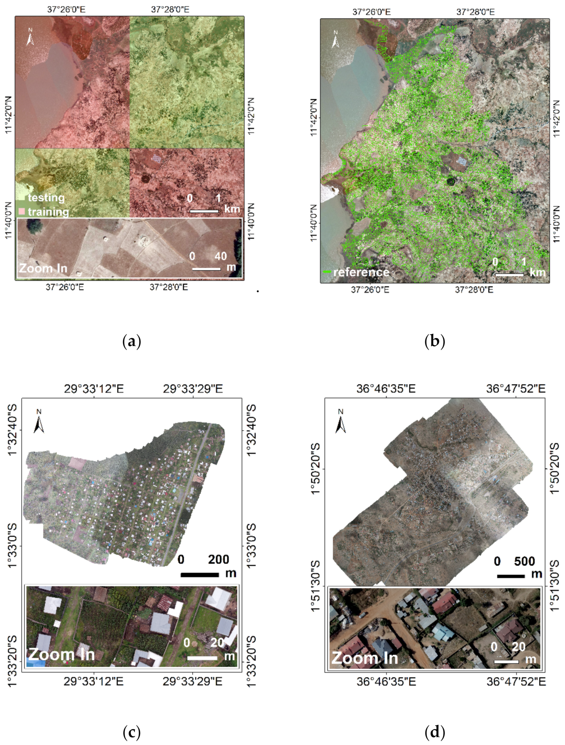
2.1. Image Data
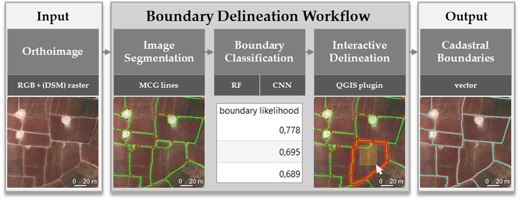
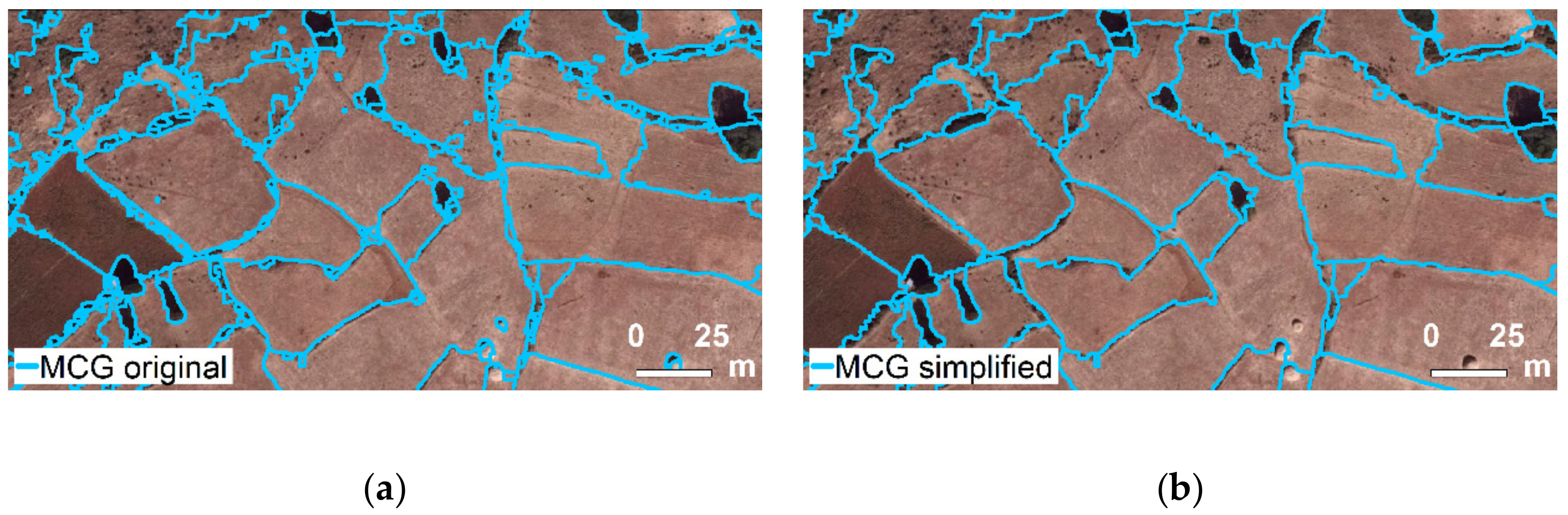
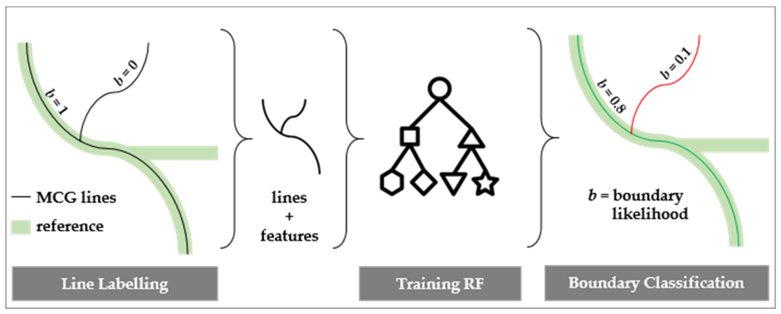
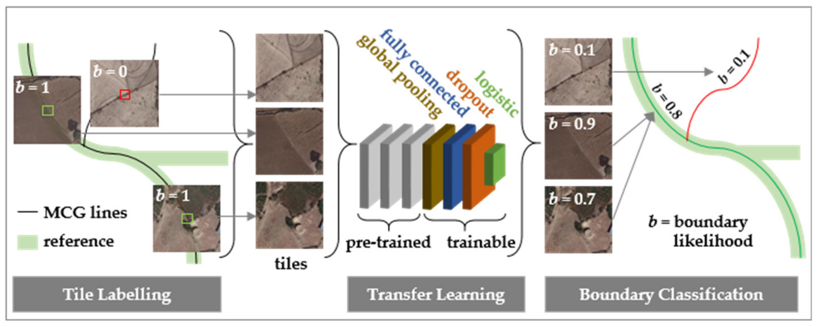
2.2. Boundary Mapping Approach
2.3. Accuracy Assessment
3. Results
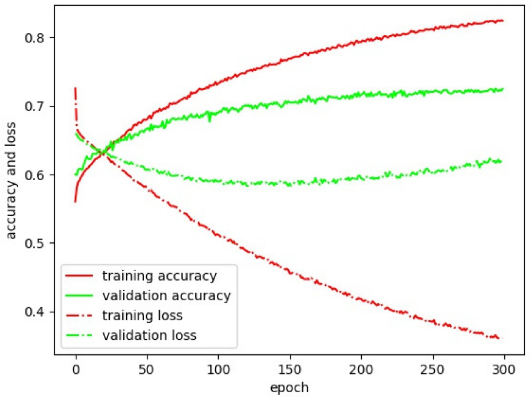
3.1. CNN Architecture
3.2. RF vs. CNN Classification
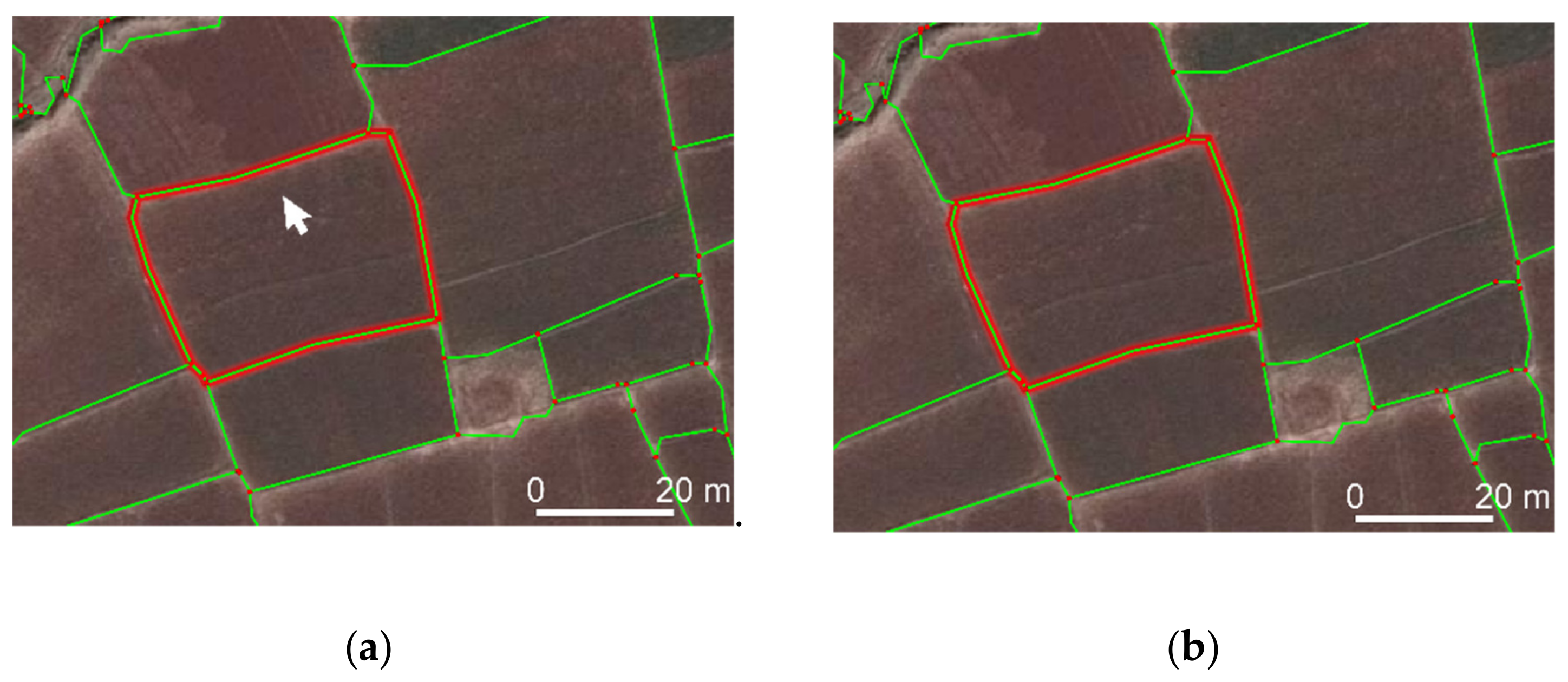
3.3. Manual vs. Automated Delineation
4. Discussion
4.1. Working Hypothesis: Improving Boundary Mapping Approach
4.2. Working Hypothesis: CNN vs. RF
4.3. Limitations & Future Work
4.4. Comparison to Previous Studies
5. Conclusions
Author Contributions
Funding
Acknowledgments
Conflicts of Interest
Appendix A

| Parameter | Value | Acc. | Loss | Plot |
|---|---|---|---|---|
| base model | VGG19 | 0.607 | 0.654 |  |
| dense layer depth | / | |||
| dense layer depth | 16 | |||
| dropout rate | 0.5 | |||
| learning rate | 0.01 | |||
| base model | VGG19 | 0.705 | 0.66 |  |
| dense layer depth | / | |||
| dense layer depth | 1024 | |||
| dropout rate | 0.5 | |||
| learning rate | 0.01 | |||
| base model | VGG19 | 0.693 | 1.632 |  |
| dense layer depth | 512 | |||
| dense layer depth | 16 | |||
| dropout rate | 0.5 | |||
| learning rate | 0.01 | |||
| base model | VGG19 | 0.613 | 0.643 |  |
| dense layer depth | / | |||
| dense layer depth | 16 | |||
| dropout rate | 0.5 | |||
| learning rate | 0.001 | |||
| base model | VGG19 | 0.615 | 0.646 |  |
| dense layer depth | / | |||
| dense layer depth | 16 | |||
| dropout rate | 0.2 | |||
| learning rate | 0.01 | |||
| base model | VGG19 | 0.6 | 0.656 |  |
| dense layer depth | 16 | |||
| dense layer depth | 16 | |||
| dropout rate | 0.8 | |||
| learning rate | 0.001 | |||
| base model | VGG16 | 0.667 | 0.608 |  |
| dense layer depth | / | |||
| dense layer depth | 1024 | |||
| dropout rate | 0.8 | |||
| learning rate | 0.001 | |||
| base model | VGG19 | 0.692 | 0.586 |  |
| dense layer depth | / | |||
| dense layer depth | 1024 | |||
| dropout rate | 0.8 | |||
| learning rate | 0.001 | |||
| base model | VGG19 | 0.733 | 1.205 |  |
| dense layer depth | / | |||
| dense layer depth | 1024 | |||
| dropout rate | 0.8 | |||
| learning rate | 0.001 | |||
| base model | ResNet50 | 0.571 | 0.742 |  |
| dense layer depth | / | |||
| dense layer depth | 16 | |||
| dropout rate | 0.5 | |||
| learning rate | 0.01 | |||
| base model | ResNet50 | 0.561 | 2.367 |  |
| dense layer depth | / | |||
| dense layer depth | 1024 | |||
| dropout rate | 0.5 | |||
| learning rate | 0.01 | |||
| base model | ResNet50 | 0.546 | 3.86 |  |
| dense layer depth | 512 | |||
| dense layer depth | 16 | |||
| dropout rate | 0.5 | |||
| learning rate | 0.01 | |||
| base model | ResNet50 | 0.577 | 0.787 |  |
| dense layer depth | / | |||
| dense layer depth | 16 | |||
| dropout rate | 0.5 | |||
| learning rate | 0.001 | |||
| base model | ResNet50 | 0.578 | 0.838 |  |
| dense layer depth | / | |||
| dense layer depth | 16 | |||
| dropout rate | 0.2 | |||
| learning rate | 0.01 | |||
| base model | InceptionV3 | 0.543 | 0.792 |  |
| dense layer depth | / | |||
| dense layer depth | 1024 | |||
| dropout rate | 0.8 | |||
| learning rate | 0.001 | |||
| base model | Xception | 0.559 | 0.777 |  |
| dense layer depth | / | |||
| dense layer depth | 1024 | |||
| dropout rate | 0.8 | |||
| learning rate | 0.001 | |||
| base model | MobileNet | 0.612 | 0.775 |  |
| dense layer depth | / | |||
| dense layer depth | 1024 | |||
| dropout rate | 0.8 | |||
| learning rate | 0.001 | |||
| base model | DenseNet201 | 0.569 | 0.895 |  |
| dense layer depth | / | |||
| dense layer depth | 1024 | |||
| dropout rate | 0.8 | |||
| learning rate | 0.001 |
References
- Enemark, S.; Bell, K.C.; Lemmen, C.; McLaren, R. Fit-for-Purpose Land Administration; International Federation of Surveyors: Frederiksberg, Denmark, 2014; p. 42. [Google Scholar]
- Williamson, I.; Enemark, S.; Wallace, J.; Rajabifard, A. Land Administration for Sustainable Development; ESRI Press Academic: Redlands, CA, USA, 2010; p. 472. [Google Scholar]
- Zevenbergen, J.; Bennett, R. The Visible Boundary: More Than Just a Line Between Coordinates. In Proceedings of the GeoTechRwanda, Kigali, Rwanda, 8–20 November 2015; pp. 1–4. [Google Scholar]
- Kohli, D.; Bennett, R.; Lemmen, C.; Asiama, K.; Zevenbergen, J. A Quantitative Comparison of Completely Visible Cadastral Parcels Using Satellite Images: A Step towards Automation. In Proceedings of the FIG Working Week 2017, Helsinki, Finland, 29 May–2 June 2017; pp. 1–14. [Google Scholar]
- Luo, X.; Bennett, R.; Koeva, M.; Lemmen, C.; Quadros, N. Quantifying the overlap between cadastral and visual boundaries: A case study from Vanuatu. Urban Sci. 2017, 1, 32. [Google Scholar] [CrossRef]
- Crommelinck, S.; Bennett, R.; Gerke, M.; Nex, F.; Yang, M.Y.; Vosselman, G. Review of automatic feature extraction from high-resolution optical sensor data for UAV-based cadastral mapping. Remote Sens. 2016, 8, 689. [Google Scholar] [CrossRef]
- Manyoky, M.; Theiler, P.; Steudler, D.; Eisenbeiss, H. Unmanned aerial vehicle in cadastral applications. In Proceedings of the International Archives of the Photogrammetry, Remote Sensing and Spatial Information Sciences, Zurich, Switzerland, 14–16 September 2011; pp. 1–6. [Google Scholar]
- Jazayeri, I.; Rajabifard, A.; Kalantari, M. A geometric and semantic evaluation of 3D data sourcing methods for land and property information. Land Use Policy 2014, 36, 219–230. [Google Scholar] [CrossRef]
- Koeva, M.; Muneza, M.; Gevaert, C.; Gerke, M.; Nex, F. Using UAVs for map creation and updating. A case study in Rwanda. Surv. Rev. 2018, 50, 312–325. [Google Scholar] [CrossRef]
- Gevaert, C.M. Unmanned Aerial Vehicle Mapping for Settlement Upgrading. Ph.D. Thesis, University of Twente, Enskede, The Netherlands, 2018. [Google Scholar]
- Maurice, M.J.; Koeva, M.N.; Gerke, M.; Nex, F.; Gevaert, C. A photogrammetric approach for map updating using UAV in Rwanda. In Proceedings of the GeoTechRwanda 2015, Kigali, Rwanda, 18–20 November 2015; pp. 1–8. [Google Scholar]
- He, H.; Zhou, J.; Chen, M.; Chen, T.; Li, D.; Cheng, P. Building extraction from UAV images jointly using 6D-SLIC and multiscale Siamese convolutional networks. Remote Sens. 2019, 11, 1040. [Google Scholar] [CrossRef]
- Marmanis, D.; Wegner, J.D.; Galliani, S.; Schindler, K.; Datcu, M.; Stilla, U. Semantic segmentation of aerial images with an ensemble of CNNs. ISPRS Ann. Photogramm. Remote Sens. Spat. Inf. Sci. 2016, 3, 473–480. [Google Scholar] [CrossRef]
- Yang, M.Y.; Liao, W.; Li, X.; Rosenhahn, B. Deep learning for vehicle detection in aerial images. In Proceedings of the IEEE International Conference on Image Processing (ICIP), Athens, Greece, 7–10 October 2018; pp. 3079–3083. [Google Scholar]
- Long, Y.; Gong, Y.; Xiao, Z.; Liu, Q. Accurate object localization in remote sensing images based on convolutional neural networks. IEEE Trans. Geosci. Remote Sens. 2017, 55, 2486–2498. [Google Scholar] [CrossRef]
- Persello, C.; Tolpekin, V.A.; Bergado, J.R.; de By, R.A. Delineation of agricultural fields in smallholder farms from satellite images using fully convolutional networks and combinatorial grouping. Remote Sens. Environ. 2019, 231, 111253. [Google Scholar] [CrossRef]
- Bergen, K.J.; Johnson, P.A.; Maarten, V.; Beroza, G.C. Machine learning for data-driven discovery in solid earth geoscience. Science 2019, 363, 0323. [Google Scholar] [CrossRef]
- Zhu, X.X.; Tuia, D.; Mou, L.; Xia, G.; Zhang, L.; Xu, F.; Fraundorfer, F. Deep learning in remote sensing: A comprehensive review and list of resources. IEEE Geosci. Remote Sens. Mag. 2017, 5, 8–36. [Google Scholar] [CrossRef]
- Ketkar, N. Deep Learning with Python; Apress: New York, NY, USA, 2017; p. 169. [Google Scholar]
- Garcia-Gasulla, D.; Parés, F.; Vilalta, A.; Moreno, J.; Ayguadé, E.; Labarta, J.; Cortés, U.; Suzumura, T. On the behavior of convolutional nets for feature extraction. J. Artif. Intell. Res. 2018, 61, 563–592. [Google Scholar] [CrossRef]
- Crommelinck, S.; Höfle, B.; Koeva, M.; Yang, M.Y.; Vosselman, G. Interactive Boundary Delineation from UAV data. In Proceedings of the ISPRS Annals of the Photogrammetry, Remote Sensing and Spatial Information Sciences, Riva del Garda, Italy, 4–7 June 2018; pp. 81–88. [Google Scholar]
- Crommelinck, S.; Koeva, M.; Yang, M.Y.; Vosselman, G. Robust object extraction from remote sensing data. arXiv 2019, arXiv:1904.12586. [Google Scholar]
- Crommelinck, S. Delineation-Tool GitHub. Available online: https://github.com/its4land/delineation-tool (accessed on 10 October 2019).
- Pont-Tuset, J.; Arbeláez, P.; Barron, J.T.; Marques, F.; Malik, J. Multiscale combinatorial grouping for image segmentation and object proposal generation. IEEE Trans. Pattern Anal. Mach. Intell. 2017, 39, 128–140. [Google Scholar] [CrossRef] [PubMed]
- Simonyan, K.; Zisserman, A. Very deep convolutional networks for large-scale image recognition. arXiv 2014, arXiv:1409.1556. [Google Scholar]
- He, K.; Zhang, X.; Ren, S.; Sun, J. Deep residual learning for image recognition. In Proceedings of the IEEE Conference on Computer Vision and Pattern Recognition (CVPR), Las Vegas, NV, USA, 26 June–1 July 2016; pp. 770–778. [Google Scholar]
- Szegedy, C.; Vanhoucke, V.; Ioffe, S.; Shlens, J.; Wojna, Z. Rethinking the inception architecture for computer vision. In Proceedings of the IEEE Conference on Computer Vision and Pattern Recognition (CVPR), Las Vegas, NV, USA, 26 June–1 July 2016; pp. 2818–2826. [Google Scholar]
- Chollet, F. Xception: Deep learning with depthwise separable convolutions. In Proceedings of the IEEE Conference on Computer Vision and Pattern Recognition (CVPR), Honolulu, HI, USA, 21–26 July 2017; pp. 1251–1258. [Google Scholar]
- Howard, A.G.; Zhu, M.; Chen, B.; Kalenichenko, D.; Wang, W.; Weyand, T.; Andreetto, M.; Adam, H. Mobilenets: Efficient convolutional neural networks for mobile vision applications. arXiv 2017, arXiv:1704.04861. [Google Scholar]
- Iandola, F.; Moskewicz, M.; Karayev, S.; Girshick, R.; Darrell, T.; Keutzer, K. Densenet: Implementing efficient convnet descriptor pyramids. arXiv 2014, arXiv:1404.1869. [Google Scholar]
- QGIS Development Team. Qgis Geographic Information System, Open Source Geospatial Foundation. Available online: https://www.qgis.org (accessed on 10 October 2019).
- Crommelinck, S. QGIS Plugin Repository: BoundaryDelineation. Available online: http://plugins.qgis.org/plugins/BoundaryDelineation/ (accessed on 10 October 2019).
- International Association of Assessing Officers (IAAO). Standard on Digital Cadastral Maps and Parcel Identifiers; International Association of Assessing Officers (IAAO): Kansas City, MO, USA, 2015; p. 24. [Google Scholar]
- Deng, J.; Dong, W.; Socher, R.; Li, L.J.; Li, K.; Li, F.F. Imagenet: A large-scale hierarchical image database. In Proceedings of the IEEE Conference on Computer Vision and Pattern Recognition (CVPR), Miami Beach, FL, USA, 20–25 June 2009; pp. 248–255. [Google Scholar]
- Chollet, F. Keras. Available online: https://keras.io (accessed on 10 October 2019).
- Nyandwi, E.; Koeva, M.; Kohli, D.; Bennett, R. Comparing Human versus Machine-Driven Cadastral Boundary Feature Extraction. Preprints 2019. [Google Scholar] [CrossRef]
- Warner, T.A.; Fang, F. Implementation of machine-learning classification in remote sensing: An applied review. Int. J. Remote Sens. 2018, 39, 2784–2817. [Google Scholar]
- Rottensteiner, F.; Sohn, G.; Jung, J.; Gerke, M.; Baillard, C.; Benitez, S.; Breitkopf, U. The ISPRS benchmark on urban object classification and 3D building reconstruction. ISPRS Ann. Photogramm. Remote Sens. Spat. Inf. Sci. 2012, 1, 293–298. [Google Scholar] [CrossRef]
- Chen, Q.; Wang, L.; Wu, Y.; Wu, G.; Guo, Z.; Waslander, S.L. Aerial imagery for roof segmentation: A large-scale dataset towards automatic mapping of buildings. ISPRS J. Photogramm. Remote Sens. 2018, 147, 42–55. [Google Scholar] [CrossRef]
- Demir, I.; Koperski, K.; Lindenbaum, D.; Pang, G.; Huang, J.; Basu, S.; Hughes, F.; Tuia, D.; Raskar, R. Deepglobe 2018: A challenge to parse the earth through satellite images. In Proceedings of the IEEE/CVF Conference on Computer Vision and Pattern Recognition Workshops (CVPRW), Salt Lake City, UT, USA, 18–22 June 2018; pp. 172–181. [Google Scholar]
- Cardim, G.; Silva, E.; Dias, M.; Bravo, I.; Gardel, A. Statistical evaluation and analysis of road extraction methodologies using a unique dataset from remote sensing. Remote Sens. 2018, 10, 620. [Google Scholar] [CrossRef]
- University of Auckland. Land Information New Zeeland Data Service. Available online: https://data.linz.govt.nz/ (accessed on 10 October 2019).
- Humanitarian OpenStreetMap Team. OpenAerialMap. Available online: https://openaerialmap.org/ (accessed on 10 October 2019).
- Debats, S.R.; Estes, L.D.; Thompson, D.R.; Caylor, K.K. Integrating active learning and crowdsourcing into large-scale supervised landcover mapping algorithms. PeerJ Prepr. 2017. [Google Scholar] [CrossRef]
- Keenja, E.; De Vries, W.; Bennett, R.; Laarakker, P. Crowd sourcing for land administration: Perceptions within Netherlands kadaster. In Proceedings of the FIG Working Week, Rome, Italy, 6–10 May 2012; pp. 1–12. [Google Scholar]
- Basiouka, S.; Potsiou, C. VGI in cadastre: A Greek experiment to investigate the potential of crowd sourcing techniques in cadastral mapping. Surv. Rev. 2012, 44, 153–161. [Google Scholar] [CrossRef]
- Moreri, K.; Fairbairn, D.; James, P. Issues in developing a fit for purpose system for incorporating VGI in land administration in Botswana. Land Use Policy 2018, 77, 402–411. [Google Scholar] [CrossRef]
- Stöcker, C.; Ho, S.; Nkerabigwi, P.; Schmidt, C.; Koeva, M.; Bennett, R.; Zevenbergen, J. Unmanned Aerial System Imagery, Land Data and User Needs: A Socio-Technical Assessment in Rwanda. Remote Sens. 2019, 11, 1035. [Google Scholar] [CrossRef]
- Spatial Collective. Mapping: (No) Big Deal. Available online: http://mappingnobigdeal.com/ (accessed on 10 October 2019).
- Crommelinck, S. Delineation-Tool Wiki. Available online: https://github.com/its4land/delineation-tool/wiki (accessed on 10 October 2019).
- Fang, L.; Cunefare, D.; Wang, C.; Guymer, R.H.; Li, S.; Farsiu, S. Automatic segmentation of nine retinal layer boundaries in OCT images of non-exudative AMD patients using deep learning and graph search. Biomed. Opt. Express 2017, 8, 2732–2744. [Google Scholar] [CrossRef]
- Long, J.; Shelhamer, E.; Darrell, T. Fully convolutional networks for semantic segmentation. In Proceedings of the IEEE Conference on Computer Vision and Pattern Recognition (CVPR), Boston, MA, USA, 7–12 June 2015; pp. 3431–3440. [Google Scholar]
- Arbeláez, P. Boundary extraction in natural images using ultrametric contour maps. In Proceedings of the Conference on Computer Vision and Pattern Recognition Workshop (CVPRW), New York, NY, USA, 17–22 June 2006; pp. 1–8. [Google Scholar]
- Volpi, M.; Tuia, D. Deep multi-task learning for a geographically-regularized semantic segmentation of aerial images. ISPRS J. Photogramm. Remote Sens. 2018, 144, 48–60. [Google Scholar] [CrossRef]
- Yang, J.; Price, B.; Cohen, S.; Lee, H.; Yang, M.H. Object contour detection with a fully convolutional encoder-decoder network. In Proceedings of the IEEE Conference on Computer Vision and Pattern Recognition (CVPR), Las Vegas, NV, USA, 26 June–1 July 2016; pp. 193–202. [Google Scholar]
- Li, P.; Zang, Y.; Wang, C.; Li, J.; Cheng, M.; Luo, L.; Yu, Y. Road network extraction via deep learning and line integral convolution. In Proceedings of the IEEE International Geoscience and Remote Sensing Symposium (IGARSS), Beijing, China, 10–15 July 2016; pp. 1599–1602. [Google Scholar]
- Zhou, W.; Wu, C.; Yi, Y.; Du, W. Automatic detection of exudates in digital color fundus images using superpixel multi-feature classification. IEEE Access 2017, 5, 17077–17088. [Google Scholar] [CrossRef]
- Kass, M.; Witkin, A.; Terzopoulos, D. Snakes: Active contour models. Int. J. Comput. Vis. 1988, 1, 321–331. [Google Scholar] [CrossRef]
- Butenuth, M.; Heipke, C. Network snakes: Graph-based object delineation with active contour models. Mach. Vis. Appl. 2012, 23, 91–109. [Google Scholar] [CrossRef]
- Gerke, M.; Butenuth, M.; Heipke, C.; Willrich, F. Graph-supported verification of road databases. ISPRS J. Photogramm. Remote Sens. 2004, 58, 152–165. [Google Scholar] [CrossRef]
- Lucas, C.; Bouten, W.; Koma, Z.; Kissling, W.D.; Seijmonsbergen, A.C. Identification of linear vegetation elements in a rural landscape using LiDAR point clouds. Remote Sens. 2019, 11, 292. [Google Scholar] [CrossRef]


| RF Classification | CNN Classification | |||
|---|---|---|---|---|
| Number of Lines | Number of Tiles | |||
| Label | Training | Testing | Training | Testing |
| ‘boundary’ | 12,280 (50%) | 9,742 (3%) | 35,643 (50%) | 34,721 (4%) |
| ‘not boundary’ | 12,280 (50%) | 280,108 (97%) | 34,665 (50%) | 746,349 (96%) |
| ∑ | 24,560 | 289,850 | 70,308 | 781,070 |
| Functionality | Description |
|---|---|
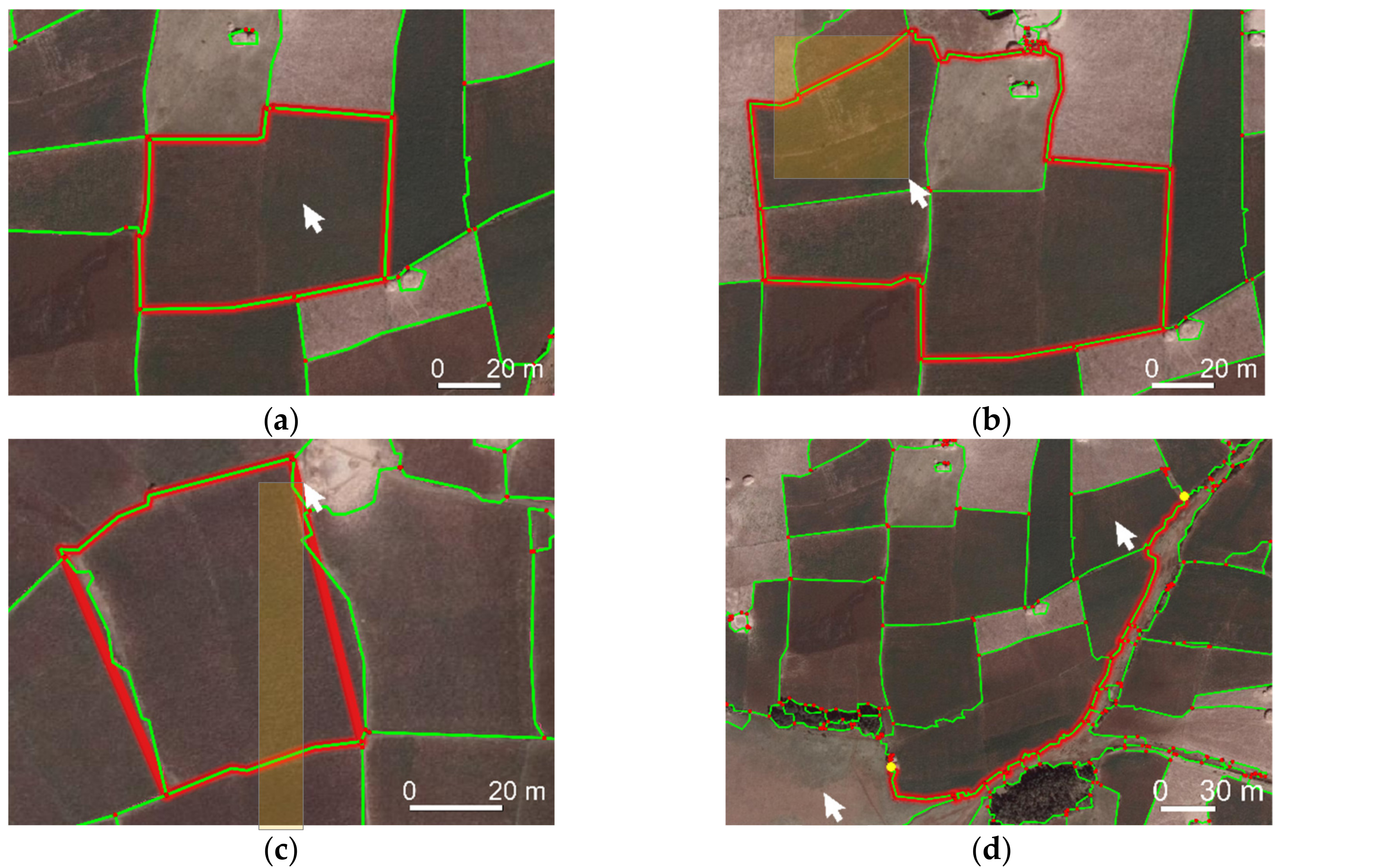
| Connect around selection | Connect lines surrounding a click or selection of lines (Figure 6a,b) |
| Connect lines’ endpoints | Connect endpoints of selected lines to a polygon, regardless of MCG lines (Figure 6c) |
| Connect along optimal path | Connect vertices along least-cost-path based on a selected attribute, e.g., boundary likelihood (Figure 6d) |
| Connect manual clicks | Manual delineation with the option to snap to input lines and vertices |
| Update edits | Update input lines based on manual edits |
| Polygonize results | Convert created boundary lines to polygons |
| Settings | Parameters | |
|---|---|---|
| untrainable layers | VGG19 pre-trained on ImageNet | exclusion of final pooling and fully connected layer |
| trainable layers | pooling layer | global average pooling 2D |
| fully connected layer | Depth = 1024, activation = ReLu | |
| dropout layer | dropout rate = 0.8 | |
| logistic layer | Activation = softmax | |
| learning optimizer | stochastic gradient descent (SGD) optimizer | learning rate = 0.001 momentum = 0.9 decay = learning rate/epochs |
| training | shuffled training tiles and un-shuffled validation tiles | Epochs = max. 200 batch size = 32 |
| Overlap | ||||||
|---|---|---|---|---|---|---|
| boundary likelihood | 0 | ]0; 1] | ∑ | ∑ % | ||
| RF | 0 | 535 | 265 | 800 | 0 | |
| ]0; 1] | 150,583 | 59,123 | 209,706 | 100 | ||
| ∑ | 151,118 | 59,388 | 210,506 | |||
| ∑ % | 72 | 28 | 100 | |||
| CNN | 0 | 7,560 | 1,794 | 9,354 | 4 | |
| ]0; 1] | 145,558 | 57,594 | 201,152 | 96 | ||
| ∑ | 151,118 | 59,388 | 210,506 | |||
| ∑ % | 72 | 28 | 100 | |||
| overlap | |||||||||
|---|---|---|---|---|---|---|---|---|---|
| 0 | ]0; 0.25] | ]0.25; 0.5] | ]0.5; 0.75] | ]0.75; 1] | ∑ | ∑ % | |||
| boundary likelihood | RF | ]0; 0.25] | 151,118 | 15,176 | 3633 | 481 | 95 | 19,385 | 32 |
| ]0.25; 0.5] | 11,553 | 5633 | 2178 | 730 | 20,094 | 34 | |||
| ]0.5; 0.75] | 6827 | 4849 | 3120 | 1617 | 16,413 | 28 | |||
| ]0.75; 1] | 973 | 1002 | 813 | 708 | 3496 | 6 | |||
| ∑ | 34,529 | 15,117 | 6592 | 3150 | 59,388 | ||||
| ∑ % | / | 58 | 26 | 11 | 5 | 100 | |||
| CNN | ]0; 0.25] | 151,118 | 26,546 | 10,472 | 4305 | 1981 | 43,304 | 73 | |
| ]0.25; 0.5] | 5974 | 3307 | 1534 | 765 | 11,580 | 19 | |||
| ]0.5; 0.75] | 1751 | 1177 | 655 | 328 | 3911 | 7 | |||
| ]0.75; 1] | 258 | 161 | 97 | 77 | 593 | 1 | |||
| ∑ | 34,529 | 15,117 | 6591 | 3151 | 59,388 | ||||
| ∑ % | / | 58 | 26 | 11 | 5 | 100 | |||
| Manual Delineation | Automated Dlineation | |||||
|---|---|---|---|---|---|---|
| Parcel Count | Parcel Count | |||||
| Ethiopia (rural) | 350 | 13 | 10 | 181 (52%) | 8 | 2 |
| Rwanda (peri-urban) | 100 | 12 | 7 | 40 (40%) | 25 | 5 |
| Kenya (peri-urban) | 272 | 11 | 5 | 157 (58%) | 10 | 4 |
| Functionality | Boundary Type | Boundary ≙ Segmentation | Example Boundary |
|---|---|---|---|
| Connect around selection | complex or rectangular | yes | agricultural field |
| Connect lines’ endpoints | small or rectangular | partly | vegetation-covered |
| Connect along optimal path | long or curved | yes | curved river |
| Connect manual clicks | fragmented or partly invisible | no or partly | low-contrast |
© 2019 by the authors. Licensee MDPI, Basel, Switzerland. This article is an open access article distributed under the terms and conditions of the Creative Commons Attribution (CC BY) license (http://creativecommons.org/licenses/by/4.0/).
Share and Cite
Crommelinck, S.; Koeva, M.; Yang, M.Y.; Vosselman, G. Application of Deep Learning for Delineation of Visible Cadastral Boundaries from Remote Sensing Imagery. Remote Sens. 2019, 11, 2505. https://doi.org/10.3390/rs11212505
Crommelinck S, Koeva M, Yang MY, Vosselman G. Application of Deep Learning for Delineation of Visible Cadastral Boundaries from Remote Sensing Imagery. Remote Sensing. 2019; 11(21):2505. https://doi.org/10.3390/rs11212505
Chicago/Turabian StyleCrommelinck, Sophie, Mila Koeva, Michael Ying Yang, and George Vosselman. 2019. "Application of Deep Learning for Delineation of Visible Cadastral Boundaries from Remote Sensing Imagery" Remote Sensing 11, no. 21: 2505. https://doi.org/10.3390/rs11212505
APA StyleCrommelinck, S., Koeva, M., Yang, M. Y., & Vosselman, G. (2019). Application of Deep Learning for Delineation of Visible Cadastral Boundaries from Remote Sensing Imagery. Remote Sensing, 11(21), 2505. https://doi.org/10.3390/rs11212505