Abstract
Scene classification is one of the bases for automatic remote sensing image interpretation. Recently, deep convolutional neural networks have presented promising performance in high-resolution remote sensing scene classification research. In general, most researchers directly use raw deep features extracted from the convolutional networks to classify scenes. However, this strategy only considers single scale features, which cannot describe both the local and global features of images. In fact, the dissimilarity of scene targets in the same category may result in convolutional features being unable to classify them into the same category. Besides, the similarity of the global features in different categories may also lead to failure of fully connected layer features to distinguish them. To address these issues, we propose a scene classification method based on multi-scale deep feature representation (MDFR), which mainly includes two contributions: (1) region-based features selection and representation; and (2) multi-scale features fusion. Initially, the proposed method filters the multi-scale deep features extracted from pre-trained convolutional networks. Subsequently, these features are fused via two efficient fusion methods. Our method utilizes the complementarity between local features and global features by effectively exploiting the features of different scales and discarding the redundant information in features. Experimental results on three benchmark high-resolution remote sensing image datasets indicate that the proposed method is comparable to some state-of-the-art algorithms.
1. Introduction
Recently, a large amount of high-resolution remote sensing images have been applied to urban functional analysis, geographic image retrieval, environment monitoring, and so on [1]. Scene classification is a fundamental work among the interpretation tasks of remote sensing images, which directly affects the subsequent interpretation of remote sensing images. Specifically speaking, the purpose of scene classification is to assign a high-level semantic label (e.g., airplane, harbor, and residential) to a local area of high-resolution remote sensing images, which is different from medium-resolution remote sensing image land use/land cover classification task [2]. Normally, scene classification consists of two parts: feature extraction and classification. Among them, it is difficult for scene classification to describe scenes better by the extracted features.
To obtain discriminative feature representation, most classification methods have focused on the research of various feature descriptors, such as histograms of oriented gradients (HOG) [3], scale-invariant feature transform (SIFT) [4], local binary patterns (LBP) [5], and GIST [6]. These feature descriptors have been extensively used in computer vision classification tasks. Unfortunately, these features are all low-level features of artificial design, containing less semantic information. There is a huge “semantic gap” between low-level features and high-level semantics of remote sensing scenes. In order to overcome the problem, researchers have proposed a scene classification approach based on mid-level features of aerial scenes. In [7], the classic Bag-of-Visual-Words (BoVW) [8] was firstly introduced into the remote sensing field, and it found that the extracted visual words can directly describe the scene content. To increase the semantic information contained in BoVW, the literature [9,10,11,12] further considered the spatial distribution between visual words. Lazebnik et al. [9] proposed a spatial pyramid model, which divided an image into different levels of the pyramid and cascaded each level of BoVW to form the final feature representation. Nevertheless, these methods only considered the absolute spatial relationship between visual words. To make up the shortcoming, a spatial co-occurrence kernel was proposed to construct relative spatial information in [10]. Moreover, the spatial pyramid version of the method was presented in [11]. The above literature used grids to integrate spatial information, which was highly sensitive to rotation of images. Therefore, a method based on a concentric circle was proposed in [12]. The method made objects of a clustering process change from conventional feature blocks to multi-scale concentric circle feature blocks. It not only enhanced scale invariance of the algorithm, but also improved the classification effect. The above approaches paid greater attention to the statistical information between local features of images and neglected the statistical correlation between visual words. Consequently, probabilistic topic models based on BoVW were developed, for instance, probabilistic Latent Semantic Analysis (pLSA) and Latent Dirichlet Allocation (LDA) models. In [13,14,15,16,17], single or multiple low-level features were firstly transformed into visual words, then modeled to mine latent topics. Furthermore, the literature [18,19] proposed a multi-feature topic model, which built topic models for different features and fused them at visual topic level.
Although mid-level feature representation can improve the classification performance of remote sensing image scenes to a certain extent, they still rely on low-level features of images and cannot realize the essential understanding of scene contents. As a result, these methods may not perform well for classifying high-resolution remote sensing images with highly complex spatial structures and extremely rich scene information [20].
In recent years, deep learning techniques, especially convolutional neural networks (ConvNets), have been widely used in remote sensing image interpretation tasks such as object detection [21,22,23], semantic segmentation [24,25,26], hyperspectral classification [27,28], and scene classification [29,30,31]. For remote sensing scene classification tasks, the existing research work shows that classification performance of algorithms based on ConvNets is significantly improved. However, ConvNets is a data-driven method, and training a new network from scratch requires a large amount of data. Currently, the scale of publicly available high-resolution remote sensing datasets is far less than the ImageNet [32], which cannot satisfy the requirement of training a novel deep ConvNets adequately. At the same time, pre-trained ConvNets based on the ImageNet present strong generalization power such as CaffeNet [33], VggNet [34], GoogLeNet [35], etc. Compared with traditional feature acquisition methods, the pre-trained ConvNets can extract more representative features. Therefore, the authors extracted the fully connected layer features of remote sensing images from pre-trained ConvNets to classify scenes in [36,37,38]. The literature [39,40,41] used the traditional feature coding methods [42,43] to encode and classify features of convolutional layers. In [44], the authors adopted a multi-scale improved fisher kernel coding method to build mid-level feature representation of convolutional features. The literature [45] used an improved Vector of Locally Aggregated Descriptors (VLAD) algorithm to encode the deep regional features for generating local feature representation of remote sensing images. To obtain robust features to objects’ scale, the literature [46,47] first fed the images with different scales produced by randomly stretching an image into ConvNets, then extracted the fully connected layer features. The discriminant correlation analysis algorithm was employed in [48] to fuse the last two fully connected layer features of pre-trained VggNet. The fusion features were regarded as the final scene representation for improving the discriminant ability. Similar to [48], the literature [49] first rearranged features of the last convolutional layer, then concatenated the fully connected layer features. Although these CNN-based approaches effectively improved the performance of remote sensing image scene classification, there are still the following limitations.
For example, most of the above research work adopts the single scale deep features (convolutional layer, etc.) or the concatenated features of convolutional and fully connected layers. The single scale deep features may be difficult to improve the scene classification performance due to containing only information of a certain scale. Besides, encoded convolutional features simply project local features to a new feature space, which perhaps loses global and spatial information of an image [49,50]. Although fusion methods of connection take into account the global and local information of images, they increase the dimension of features. These methods may not utilize the complementary information of different layers from ConvNets effectively.
To address the aforementioned problems, we propose a scene classification approach based on multi-scale deep feature representation (MDFR). The proposed approach integrates the local information at complementary feature maps based on feature maps selection algorithm and region covariance descriptor. In addition, considering the limitation of single scale features, we further fuse deep features of multiple convolutional and fully connected layers via a multi-scale fusion strategy.
The major contributions of this paper can be summarized as follows:
- We propose a feature maps selection algorithm to choose the complementary feature maps. Meanwhile, we combine the region covariance descriptor to fuse feature maps of different layers. The fused deep local features may enhance local information and achieve higher discrimination with lower feature dimension.
- We develop a new feature fusion strategy to integrate the multi-scale deep features, which effectively merge the local and global information of images in remote sensing image scene classification task.
2. Proposed Method
In this section, we will elaborate each part of our algorithm in more details. The MDFR framework based feature level fusion is illustrated in Figure 1.
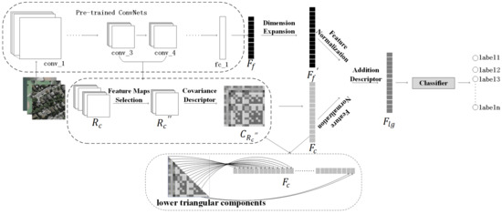
Figure 1.
Overall architecture of the proposed method. Firstly, we extract multiple deep features from the pre-trained ConvNets. Secondly, process deep local features via feature maps selection algorithm and region descriptor. Finally, use an addition descriptor to fuse the two stream features and achieve classification.
Our framework is composed of three components. Firstly, multiple deep features are extracted by the pre-trained CaffeNet. The architecture of CaffeNet comprises five convolutional layers, each followed by a pooling layer, and three fully connected layers at the end. Compared with VggNet, GoogLeNet, etc, it has fewer layers. Nevertheless, the deeper the pre-trained ConvNets is, the more dependent the extracted features are on the original dataset (ImageNet), which may result in worse performance for classifying aerial scenes [51]. For this reason, our model proposed in this paper adopts pre-trained CaffeNet for high-resolution remote sensing scenes. Secondly, a feature maps selection algorithm based on the complementarity of feature maps is proposed to choose the effective feature maps. Meanwhile, the region covariance descriptor is combined to process multiple feature maps. Finally, we develop an addition descriptor to further fuse the deep local and global features.
2.1. Deep Local Feature Representation
Unlike natural images, the shooting angle of remote sensing scenes is usually a top-down perspective. As a result, there is no definite spatial relationship between the distribution of scene objects. In this paper, the output values of the third layer (conv_3) and the fourth layer (conv_4) from CaffeNet are regarded as the local features of scenes so as to make local information more correct and complete. In addition, the feature maps selection algorithm is proposed to filter multiple feature maps of different convolutional layers and region covariance descriptor fuses the selected feature maps for improving the discrimination of deep local features.
2.1.1. Covariance as a Region Descriptor
Let R denote a rectangular region, and be the D-dimensional feature points within the range of R. Then the calculation formula of covariance descriptor [52] in region R is as follows:
where is the mean of D-dimensional feature points ,
as the feature representation of region R has the following three advantages: (1) By calculating the covariance matrix to fuse correlated multiple features, the fusion of any two feature maps at relevant positions can be achieved. Compared with unfused features, the representation ability of fused features is greatly enhanced; (2) The covariance matrix is independent from the order of feature points, and the fusion features have a certain scale and rotation invariance; (3) The covariance matrix has symmetry, which effectively relieves the problem of higher feature dimensions. In this paper, conv_3 feature maps and conv_4 feature maps are firstly connected to construct region . Then, the region covariance descriptor of is obtained. The schematic of and fusion of different feature points are shown in Figure 2, where is the number of feature maps. (, ) is the fusion result of any two feature maps. According to CaffeNet, the size of is 13 × 13 × 768. If the covariance matrix of is calculated directly, the redundant information between feature maps may weaken the discrimination of local features. Besides, the dimension of features will also be close to 300 k and the computational complexity seems to be high for the final classification.
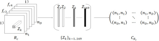
Figure 2.
and fusion process of different feature points.
2.1.2. Feature Maps Selection Algorithm
To address the aforementioned limitations, the feature maps selection algorithm is proposed. Moreover, for guaranteeing the algorithm simple and feasible, and are equally divided into n groups according to a channel-wise average fusion method [53]. The average feature map of each group is calculated in Equation (3).
In Equation (3), denotes the element of average feature matrix at and is the number of feature maps. represents the average function. Then, all average feature maps are combined into a new in the original order. Aiming at the redundant information existing in , the following algorithm is designed: first of all, execute the region covariance descriptor, of and transform into the Euclidean space in Equation (4).
where V is the decomposition matrix of [54]. Secondly, all feature values in the lower triangular of are rearranged into one-dimensional vector. The vector representing each image is then fed the SVM classifier and record the classification accuracy. Thirdly, the average feature maps are selected based on the complementarity of feature maps. The overall algorithm is summarized in Algorithm 1.
| Algorithm 1: Feature Maps Selection. |
| Input: |
| average feature maps, ; |
| Output: |
| selected feature maps, ; |
| 1: Calculate the region covariance descriptor of ; |
| 2: Transform into in Equation (4); |
| 3: Rearrange all feature values in the lower triangular of into one-dimensional vector ; |
| 4: Train a classifier on set to record the classification accuracy; |
| 5: Calculate covariance matrix () of feature map (i=1...2n); |
| 6: Repeat 2,3,4, and record the number k of corresponding feature map; |
| 7: Sort the accuracy records obtained in 6 in descending order; |
| 8: Select feature maps whose accuracies are lower than the accuracy obtained in 4; |
| 9: Construct the final ; |
| 10: return ; |
2.2. Deep Global Feature Representation
To better fuse multi-scale deep features, we extract features of the first fully connected layer. The output of the first fully connected layer is a Q-dimensional vector, as formulated in Equation (5). Among them, is the global feature, and denotes the feature maps of the last convolutional layer. and represent the matrix of weight and threshold respectively. is the key of the ConvNets, and it can be acquired through supervised learning. A nonlinear function is provided in . In fact, there are a lot of activation functions for selection. We employ the Rectified Linear Unit in the processing unit, which is reflected in Equation (6).
where and are the output and input of j-th neuron in the first fully connected layer, respectively. Since local and global features belong to different data distributions, data normalization of and are carried out before feature fusion. Taking as an example, it is assumed that a dataset contained m samples. According to the network architecture, it can be known that the dimension of is 4096 and the size of the global feature matrix composed of m samples is . Each column in represents all dimensions of the global features of a sample, and each row represents the same dimension of the global features of all samples. In this paper, each row of global feature matrix is normalized, and the data normalization is expressed as follows:
where , represent the features before and after normalization, respectively. and are the maximum and minimum values of the same dimension i from feature matrix . It is worth noting that when all values of a certain dimension are the same, is equal to . The divisor of Equation (8) is zero. As a result, all values of this dimension are retained for whole samples.
2.3. Feature Fusion and Classification
In this paper, we propose a feature fusion algorithm based on element-wise addition descriptor to fuse the two stream features of the model. The calculation formula of addition descriptor is as follows:
In Equation (9), is the final feature representation, and “⊕” represents the summation function. , are i-th element of the final local and global features, respectively. denotes the weight coefficient and the dimension of is denoted as D.
Owing to inconsistency of feature dimensions at different scales, this paper proposes using zero elements to expand the features with lower dimension.
Compared with concatenation, our method reduces the dimension of . Moreover, the experimental results demonstrate that the classification accuracy of fusion features obtained by our method is better than both the single scale features and other fusion features.
In the classification task, we use LIBSVM library [55] to realize supervised classification. The linear function is selected as the kernel function, and the regularization parameter C is determined by fivefold cross validation with the arrangement of [].
3. Experiments
To evaluate the effectiveness of the proposed approach, we conducted experiments on three public datasets. All experiments were performed in a MATLAB R2016a environment on a PC with 3.0 GHz i5-7400 CPU and 16 GB memory. Moreover, a GPU of NVIDIA GTX 1080Ti is used to increase the computing speed.
3.1. Data Sets Description
3.1.1. UC-Merced Data Set (UCM)
The UCM [10] dataset consists of 21 classes of land-use images with a pixel resolution of one foot. The original images were downloaded from the United States Geological Survey (USGS) National Map of the following US regions: Birmingham, Boston, Buffalo, Columbus, Dallas, Harrisburg, Houston, Jacksonville, Las Vegas, Los Angeles, Miami, Napa, New York, Reno, San Diego, Santa Barbara, Seattle, Tampa, Tucson, and Ventura. The size of each image is pixels. The dataset contains 2100 images with 100 samples for each class. Some examples of the UCM dataset are shown in Figure 3. Even though the dataset is small in scale, it is extremely challenging due to its higher intraclass variations (tennis courts, forests, etc.) and smaller interclass dissimilarity (building, dense residential, medium density residential, sparse residential, mobile home park, etc.).
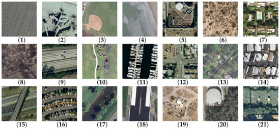
Figure 3.
Sample images of the UCM dataset: (1) Agricultural, (2) Airplane, (3) Baseball diamond, (4) Beach, (5) Building, (6) Chaparral, (7) Dense residential, (8) Forest, (9) Freeway, (10) Golf course, (11) Harbor, (12) Intersection, (13) Medium residential, (14) Mobile-homepark, (15) Overpass, (16) Parking lot, (17) River, (18) Runway, (19) Sparse residential, (20) Storage tanks, (21) Tennis court.
3.1.2. AID Data Set
The images of AID [51] dataset were collected from the Google Earth Imagery. The dataset has 10,000 images distributed on 30 aerial scene classes and the image number of each class varies from 220 to 420. The size of each image is pixels, and the pixel resolution changes from about 8 to 0.5 m. In the public scene datasets, the AID dataset is large in scale and difficult for classifying. Some examples of AID dataset are presented in Figure 4.
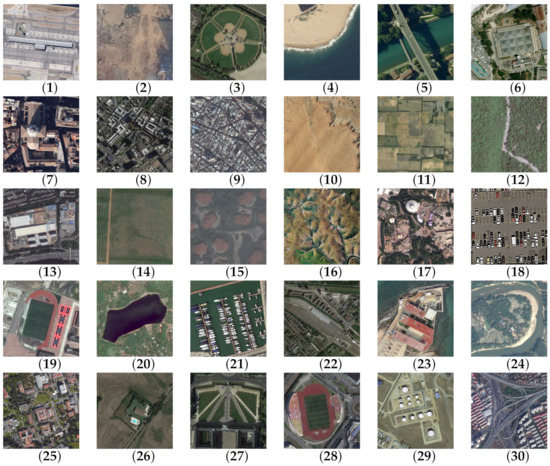
Figure 4.
Sample images of the AID dataset: (1) Airport, (2) Bare land, (3) Baseball field, (4) Beach, (5) Bridge, (6) Center, (7) Church, (8) Commercial, (9) Dense residential, (10) Desert, (11) Farmland, (12) Forest, (13) Industrial, (14) Meadow, (15) Medium residential, (16) Mountain, (17) Park, (18) Parking lot, (19) Playground, (20) Pond, (21) Port, (22) Railway station, (23) Resort, (24) River, (25) School, (26) Sparse residential, (27) Square, (28) Stadium, (29) Storage tanks, (30) Viaduct.
3.1.3. NWPU-RESISC45 Data Set (NWPU/NWPU45)
The NWPU [1] dataset includes totally 31,500 scenes divided into 45 classes. All scenes were obtained from the Google Earth Imagery. Each class consists of 700 images with a size of pixels. Except for islands, lakes, mountains and snow bergs, the spatial resolution of other scenes varies from 0.2 to 30 m. In comparison, this dataset possesses more abundant variations in viewpoint, object pose, appearance, illumination, and background, etc, within the same class, and there is a high semantic overlap between classes. Some examples are shown in Figure 5.
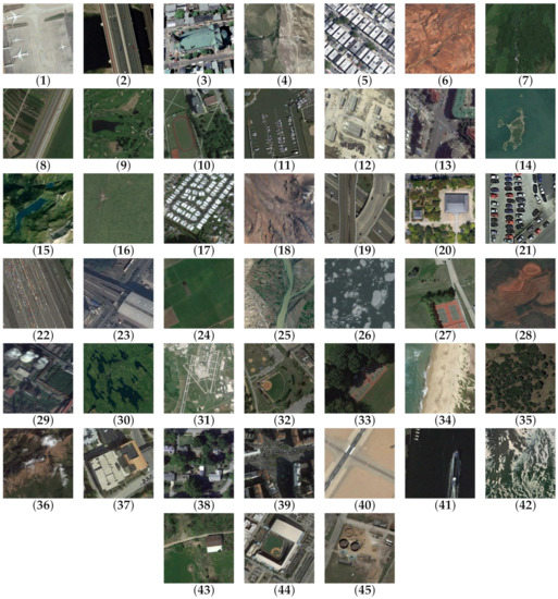
Figure 5.
Sample images of the NWPU dataset: (1) Airplane, (2) Bridge, (3) Church, (4) Circular_farmland, (5) Dense_residential, (6) Desert, (7) Forest, (8) Freeway, (9) Golf_course, (10) Ground_track_field, (11) Harbor, (12) Industrial_area, (13) Intersection, (14) Island, (15) Lake, (16) Meadow, (17) Mobile_home_park, (18) Mountain, (19) Overpass, (20) Palace, (21) Parking_lot, (22) Railway, (23) Railway_station, (24) Rectangular_farmland, (25) River, (26) Sea_ice, (27) Tennis_court, (28) Terrace, (29) Thermal_power_station, (30) Wetland, (31) Airport, (32) Baseball_diamond, (33) Basketball_court, (34) Beach, (35) Chaparral, (36) Cloud, (37) Commercial_area, (38) Medium_residential, (39) Roundabout, (40) Runway, (41) Ship, (42) Snowberg, (43) Sparse_residential, (44) Stadium, (45) Storage_tank.
3.2. Experimental Setup
3.2.1. Data Preprocessing
In this work, to ensure a fair comparison, we used the same ratio as the literatures [39,41,49,51,53] to divide each dataset. For the UCM dataset, we set the training ratio to 80%, and the rest for testing. Besides, all training samples of UCM dataset are further divided into 80% training data and 20% validation data. For the AID dataset, we set two training ratios, 20% and 50%, respectively. Similarly, 10% and 20% training ratio are used for the NWPU dataset. Because of the fixed image size required by the pre-trained ConvNets, all images are resized to pixels with bicubic interpolation.
3.2.2. Evaluation Metrics
To obtain reliable results, each experiment is tested for 30 times to reduce the influence of the randomness. We select the overall accuracy (OA), standard deviation (Std), confusion matrix and average accuracy (AA) as evaluation metrics. AA is the classification accuracy of each class.
3.2.3. Parameters Setting
The parameters affect the final classification performance of the model. In this paper, we mainly validate three hyperparameters via a lot of experiments. Among them, represents selected convolutional layers. C and are the regularization parameter of the classifier and weight coefficient, respectively.
3.2.4. Experiments Design
Firstly, the fusion effect of different convolutional layers is analyzed to determine the fusion layers and the parameter selection is discussed. Then, we compare and analyze the visualization results of the feature map selection algorithm. Thirdly, the effectiveness of fusion method and the superiority of the MDFR model are validated by comparing with other scene classification methods. Finally, a paired t-test statistical analysis is performed.
3.3. Analysis of Fusion Effects of Different Convolutional Layers
In order to improve the classification accuracy and reduce the dimension of final local features as much as possible, this paper fuses the features of different convolutional layers. The experiment consists of one convolutional layer, two convolutional layers and three convolutional layers. The UCM dataset is used for all experiments. The results are presented in Table 1. Among them, “c_m” represents features of m-th convolutional layer and “c_m_n” is the fusion features of m-th and n-th convolutional layer, and so on. From the results, we can observe that the features of low convolutional layers (c_1 and c_2) are obviously inferior to those of middle and high convolutional layers (c_3, c_4, c_5) and the fusion features. Different convolutional layers, especially the middle and high layers, can improve the recognition ability of local features. Considering the dimension of features and classification performance, the MDFR model proposed in this paper selects conv_3 and conv_4 for local feature fusion.

Table 1.
Classification accuracy of different convolutional layers (%).
3.4. Parameter Selection
The parameter in Equation (9) is the weight coefficient of deep local features. In order to find the best parameter for the classification task, we perform the comparative experiment on the representative UCM dataset. Figure 6 shows the results of different by the proposed method. In the experiment, varies from 0.1 to 0.9. It can be seen from Figure 6 that the classification accuracy is gradually improved when increases from 0.1 to 0.6. However, the classification accuracy reduces when continues to grow. Therefore, is set to 0.6 in this paper for weighted fusion of the global and local features. The experimental result further indicates that multi-scale features improve the accuracy of remote sensing image scene classification.
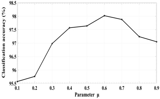
Figure 6.
Classification performance of the proposed MDFR framework with different parameter .
3.5. Comparative Analysis of Feature Maps Selection Algorithm
In order to verify the effectiveness of feature maps selection algorithm, in this paper, we use the t-sne algorithm to visualize the features before and after selection. The categories of UCM and AID dataset are presented in Table 2 and Table 3.
Table 2.
The number of features and categories on the UCM dataset.
Table 3.
The number of features and categories on the AID dataset.
Figure 7 shows the two-dimensional distribution of different features. Among them, Figure 7a,b present the visualization results of UCM dataset and AID dataset, respectively. In Figure 7a,b, the same mark represents the same category. To analyze intraclass clustering and interclass separation, we select some categories that are easy to compare. In Figure 7, we cover the same category as much as possible with a circle. In terms of coverage, the deep features after selection are more compact in the same category, and the confusion of different categories are obviously weaker than the features before selection. The comparative results show that the feature maps selection algorithm proposed in this paper can improve the discrimination of features. Besides, some categories (e.g., #12, #13, and #21 in Figure 7a) are relatively confused, which also indicates that the single scale features have a certain limitation.
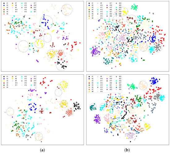
Figure 7.
Visualization results of different datasets. (a) UCM dataset. (b) AID dataset. The top figures show the features before selection and the bottom figures show the features after selection.
3.6. Analysis and Discussion
In this part, the experiments of low-level features, mid-level features and high-level features are performed respectively. Table 4 illustrates the means of OAs using the different features on UCM dataset. Among them, SIFT and CH features are selected as the low-level features. In addition, they are coded by IFK to obtain the mid-level features. High-level feature and represent the local and global features obtained by our method, respectively. By comparing the results of different feature representation, the fusion features of and give the best performance. Moreover, the classification accuracy of SIFT ⊕ CH is higher than that of SIFT and CH 29.98% and 16.25% and the classification accuracy of IFK(SIFT) ⊕ IFK(CH) is higher than IFK(SIFT) and IFK(CH) 8.39% and 10.09%, respectively. The results indicate that the fusion method is applicable to features of different level.
Table 4.
Classification accuracies of different features. The best result is in bold.
To further verify the effectiveness of this method, we compare it with other scene classification methods. Since our method uses multiple fusion methods to enhance the representation power of multi-scale deep features extracted from ConvNets, we mainly compare our method with CNN-based and other fusion methods on UCM, AID and NWPU dataset. The comparison results are shown as follows.
In Table 5, we report the overall accuracies for all these comparable methods, as they are contained in the original papers, together with the accuracy of our proposed method. The classification accuracy (98.02%) obtained by our method on UCM is higher than the CaffeNet [51], Scenario(II) [39] based on single scale deep features, and GLDFB [41], GLM16 [49], AlexNet + MSCP [53] based on other fusion methods. Figure 8 shows the confusion matrix (a) based on the UCM dataset and all samples (b) of misclassification in the testing set, respectively. The confusion matrix is the result of one of the experiments. From the confusion matrix of UCM (Figure 8), we can observe that classification accuracies of only three categories are less than 100%. Analyzing the misclassified images, we can find that the interclass distances of confused categories are extremely small. For example, overpass, intersection, and freeway. There are only slight differences in the structural relationships. Nevertheless, the average classification accuracy of all scene categories (21 categories) on UCM dataset also reaches 98.57%, which demonstrates the superiority of our method.
Table 5.
Comparison of classification accuracy with other methods (UCM). The best result is in bold.
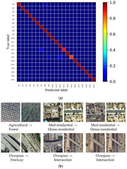
Figure 8.
Confusion matrix and all misclassification examples for the UCM dataset using the proposed MDFR architecture. (a) Confusion matrix of the UCM dataset with OA = 98.57%. (b) Misclassified samples of the UCM dataset.
Similar to the experiments discussed above for UCM dataset, we evaluate the classification performance on the AID and NWPU dataset. We follow the experimental setup employed in [53]. Table 6 displays the experimental results on the AID and NWPU dataset. As can be seen, on AID dataset, our MDFR model achieves better performance than CaffeNet [51] and VGG-VD-16 [51]. Specifically, it improves the performance by nearly 4% in terms of OA, and the OA exceeds 90% when the training set only has 20% data. Similarly, the classification accuracy of our method on the NWPU dataset is also higher than CaffeNet [51], AlexNet [1] and Fine-tuned GoogLeNet [1] by 5%, 7% and 0.8%, respectively. Compared with AlexNet+MSCP [51], our method improves the OAs of two datasets. Moreover, our feature size is reduced to about one third of its features, which greatly improves the classification performance of our model. Figure 9 and Figure 10 show the confusion matrix and some samples of misclassification based on AID and NWPU dataset, respectively. The confusion matrix is the result of one of the experiments. As can be seen from the confusion matrix, the classification accuracies of 17 scene categories in AID dataset are more than 95%, and that of 31 scene categories in NWPU dataset are more than 85%. However, according to some samples of misclassification, it is difficult to distinguish some categories with similar spatial structure, such as resort and park, center and square in the AID dataset, palaces and churches, basketball courts and tennis courts, mountain and desert in the NWPU dataset. The MDFR model still has some room for improvement in the recognition of these categories.
Table 6.
Comparison of classification accuracy with other methods. The best results are in bold.
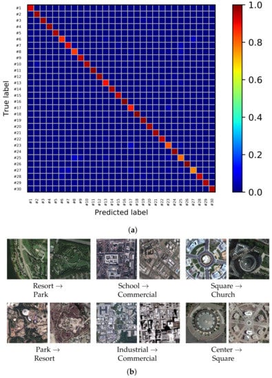
Figure 9.
Confusion matrix and some misclassification examples for the AID dataset using the proposed MDFR architecture. (a) Confusion matrix of the AID dataset with OA = 93.64%. (b) Some misclassified samples of the AID dataset.
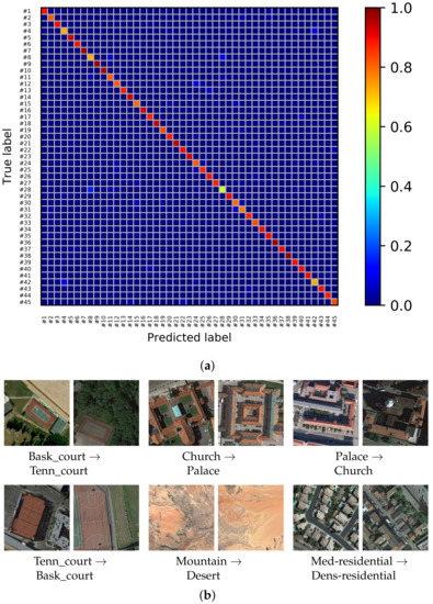
Figure 10.
Confusion matrix and some misclassification examples for the NWPU dataset using the proposed MDFR architecture. (a) Confusion matrix of the NWPU dataset with OA = 86.89%. (b) Some misclassified samples of the NWPU dataset.
Based on the experimental results in Table 5 and Table 6, we performed paired t-test experiments to further analyze the OAs of different methods. t-test is a popular statistical approach which can better validate the significance between two groups of data. It is expressed as follows:
where and represent the OAs of the two comparison methods, and are the corresponding standard deviations, and are the number of repeated experiments (, = 30), and is the significance level. In order to get reliable results, we statistically analyze our method, CaffeNet and AlexNet + MSCP that performs better on three datasets. The OAs of 30 experiments using different algorithms are presented in Figure 11. In a box plot, the red line denotes the median of OAs. The t-test results of three datasets indicate that there is significant differences between MDFR and other algorithms (at level 95%).
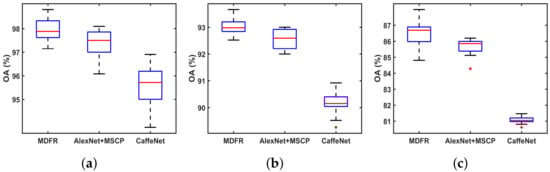
Figure 11.
Box plots of different methods. From top to the bottom are the plots by (a) UCM, (b) AID, (c) NWPU.
4. Conclusions
In this paper, we proposed a multi-scale deep feature representation framework for remote sensing image scene classification. In our method, multiple feature maps of different convolutional layers are firstly filtered by the feature maps selection algorithm. Then, the region covariance descriptor fuses the local information of corresponding positions at the complementary feature maps. Furthermore, to improve the discrimination of scene features, we develop an addition descriptor to integrate the deep local features and global features. The main contributions of the proposed approach are: (1) The representation power of deep local features may be enhanced by combining feature maps selection algorithm with region covariance descriptor. (2) The proposed feature fusion strategy merges the information of different scales in remote sensing images.
To verify the classification performance of the proposed MDFR algorithm, extensive experiments were performed on three challenging remote sensing scene datasets. Experimental results demonstrate that our approach improves the accuracies in contrast to other methods. Nevertheless, the proposed method in this paper is still not ideal for a few categories with small interclass distance and may not be applicable to heterogenous landscapes. In the future, we will pay more attention to improving the discrimination of deep features, and studying scene classification methods on remote sensing imagery with different spatial resolutions.
Author Contributions
Investigation, J.Z., M.Z.; methodology, J.Z., M.Z.; writing–original draft preparation, M.Z.; writing–review and editing, L.S., W.Y., B.P.; funding acquisition, L.S., W.Y.
Funding
This work was supported by the National Natural Science Foundation of China (Grant No. 61702157), and the Natural Science Foundation of Hebei Province (Grant No. F2017202145).
Acknowledgments
The authors would like to thank Shawn Newsam from the University of California at Merced, Guisong Xia from Wuhan University and Gong Cheng from Northwestern Polytechnical University, for providing the UCM, AID and NWPU datasets in their study, respectively.
Conflicts of Interest
The authors declare no conflict of interest.
References
- Cheng, G.; Han, J.; Lu, X. Remote sensing image scene classification: Benchmark and state of the art. Proc. IEEE 2017, 105, 1865–1883. [Google Scholar] [CrossRef]
- Abdullah, A.Y.; Masrur, A.; Adnan, M.S.; Baky, M.; Al, A.; Hassan, Q.K.; Dewan, A. Spatio-Temporal Patterns of Land Use/Land Cover Change in the Heterogeneous Coastal Region of Bangladesh between 1990 and 2017. Remote Sens. 2019, 11, 790. [Google Scholar] [CrossRef]
- Dalal, N.; Triggs, B. Histograms of oriented gradients for human detection. In Proceedings of the International Conference on Computer Vision and Pattern Recognition (CVPR’05), San Diego, CA, USA, 20–25 June 2005; Volume 1, pp. 886–893. [Google Scholar]
- Lowe, D.G. Distinctive image features from scale-invariant keypoints. Int. J. Comput. Vis. 2004, 60, 91–110. [Google Scholar] [CrossRef]
- Ojala, T.; Pietikäinen, M.; Mäenpää, T. Multiresolution gray-scale and rotation invariant texture classification with local binary patterns. IEEE Trans. Pattern Anal. Mach. Intell. 2002, 7, 971–987. [Google Scholar] [CrossRef]
- Oliva, A.; Torralba, A. Modeling the shape of the scene: A holistic representation of the spatial envelope. Int. J. Comput. Vis. 2001, 42, 145–175. [Google Scholar] [CrossRef]
- Weizman, L.; Goldberger, J. Urban-area segmentation using visual words. IEEE Geosci. Remote Sens. Lett. 2009, 6, 388–392. [Google Scholar] [CrossRef]
- Fei-Fei, L.; Perona, P. A bayesian hierarchical model for learning natural scene categories. In Proceedings of the 2005 IEEE Computer Society Conference on Computer Vision and Pattern Recognition (CVPR’05), San Diego, CA, USA, 20–25 June 2005; Volume 2, pp. 524–531. [Google Scholar]
- Lazebnik, S.; Schmid, C.; Ponce, J. Beyond bags of features: Spatial pyramid matching for recognizing natural scene categories. In Proceedings of the IEEE Conference on Computer Vision and Pattern Recognition, New York, NY, USA, 17–22 June 2006; pp. 2169–2178. [Google Scholar]
- Yang, Y.; Newsam, S. Bag-of-visual-words and spatial extensions for land-use classification. In Proceedings of the SIGSPATIAL International Conference on Advances in Geographic Information Systems, San Jose, CA, USA, 2–5 November 2010; pp. 270–279. [Google Scholar]
- Yi, Y.; Newsam, S. Spatial pyramid co-occurrence for image classification. In Proceedings of the IEEE International Conference on Computer Vision, Barcelona, Spain, 6–13 November 2011; pp. 1465–1472. [Google Scholar]
- Zhao, L.-J.; Tang, P.; Huo, L.-Z. Land-use scene classification using a concentric circle-structured multiscale bag-of-visual-words model. IEEE J. Sel. Top. Appl. Earth Obs. Remote Sens. 2014, 7, 4620–4631. [Google Scholar] [CrossRef]
- Lienou, M.; Maitre, H.; Datcu, M. Semantic annotation of satellite images using latent dirichlet allocation. IEEE Geosci. Remote Sens. Lett. 2010, 7, 28–32. [Google Scholar] [CrossRef]
- Hu, F.; Yang, W.; Chen, J.; Sun, H. Tile-level annotation of satellite images using multi-level max-margin discriminative random field. Remote Sens. 2013, 5, 2275–2291. [Google Scholar] [CrossRef]
- Luo, W.; Li, H.; Liu, G. Automatic annotation of multispectral satellite images using author-topic model. IEEE Geosci. Remote Sens. Lett. 2012, 9, 634–638. [Google Scholar]
- Luo, W.; Li, H.; Liu, G.; Zeng, L. Semantic annotation of satellite images using author-genre-topic model. IEEE Trans. Geosci. Remote Sens. 2014, 52, 1356–1368. [Google Scholar] [CrossRef]
- Zhu, Q.; Zhong, Y.; Wu, S.; Zhang, L.; Li, D. Scene classification based on the sparse homogeneous– heterogeneous topic feature model. IEEE Trans. Geosci. Remote Sens. 2018, 56, 2689–2703. [Google Scholar] [CrossRef]
- Zhong, Y.; Cui, M.; Zhu, Q.; Zhang, L. Scene classification based on multifeature probabilistic latent semantic analysis for high spatialresolution remote sensing images. J. Appl. Remote Sens. 2015, 9, 095064. [Google Scholar] [CrossRef]
- Zhong, Y.; Zhu, Q.; Zhang, L. Scene classification based on the multifeature fusion probabilistic topic model for high spatial resolution remote sensing imagery. IEEE Trans. Geosci. Remote Sens. 2015, 53, 6207–6222. [Google Scholar] [CrossRef]
- Li, X.; Shi, J.; Dong, Y.; Tao, D. Overview of scene image classification technology. Chin. Sci. Inf. Sci. 2015, 45, 827–848. [Google Scholar]
- Wang, C.; Bai, X.; Wang, S.; Zhou, J.; Ren, P. Multiscale visual attention networks for object detection in VHR remote sensing images. IEEE Geosci. Remote Sens. Lett. 2018, 16, 310–314. [Google Scholar] [CrossRef]
- Yang, X.; Sun, H.; Fu, K.; Yang, J.; Sun, X.; Yan, M.; Guo, Z. Automatic ship detection in remote sensing images from google earth of complex scenes based on multiscale rotation dense feature pyramid networks. Remote Sens. 2018, 10, 132. [Google Scholar] [CrossRef]
- Li, K.; Cheng, G.; Bu, S.; You, X. Rotation-insensitive and context-augmented object detection in remote sensing images. IEEE Trans. Geosci. Remote Sens. 2017, 56, 2337–2348. [Google Scholar] [CrossRef]
- Sun, W.; Wang, R. Fully convolutional networks for semantic segmentation of very high resolution remotely sensed images combined with DSM. IEEE Geosci. Remote Sens. Lett. 2018, 15, 474–478. [Google Scholar] [CrossRef]
- Audebert, N.; Le Saux, B.; Lefèvre, S. Segment-before-detect: Vehicle detection and classification through semantic segmentation of aerial images. Remote Sens. 2017, 9, 368. [Google Scholar] [CrossRef]
- Sherrah, J. Fully convolutional networks for dense semantic labelling of high-resolution aerial imagery. arXiv 2016, arXiv:1606.02585. [Google Scholar]
- Pan, B.; Shi, Z.; Xu, X.; Shi, T.; Zhang, N.; Zhu, X. CoinNet: Copy Initialization Network for Multispectral Imagery Semantic Segmentation. IEEE Geosci. Remote Sens. Lett. 2019, 16, 816–820. [Google Scholar] [CrossRef]
- Xu, X.; Shi, Z.; Pan, B.; Li, X. A Classification-Based Model for Multi-Objective Hyperspectral Sparse Unmixing. IEEE Trans. Geosci. Remote Sens. 2019. [Google Scholar] [CrossRef]
- Liu, Y.; Huang, C. Scene classification via triplet networks. IEEE J. Sel. Top. Appl. Earth Obs. Remote Sens. 2017, 11, 220–237. [Google Scholar] [CrossRef]
- Cheng, G.; Yang, C.; Yao, X.; Guo, L.; Han, J. When deep learning meets metric learning: Remote sensing image scene classification via learning discriminative CNNs. IEEE Trans. Geosci. Remote Sens. 2018, 56, 2811–2821. [Google Scholar] [CrossRef]
- Yu, Y.; Liu, F. Dense connectivity based two-stream deep feature fusion framework for aerial scene classification. Remote Sens. 2018, 10, 1158. [Google Scholar] [CrossRef]
- Russakovsky, O.; Deng, J.; Su, H.; Krause, J.; Satheesh, S.; Ma, S.; Huang, Z.; Karpathy, A.; Khosla, A.; Bernstein, M.; et al. Imagenet large scale visual recognition challenge. Int. J. Comput. Vis. 2015, 115, 211–252. [Google Scholar] [CrossRef]
- Jia, Y.; Shelhamer, E.; Donahue, J.; Karayev, S.; Long, J.; Girshick, R.; Guadarrama, S.; Darrell, T. Caffe: Convolutional architecture for fast feature embedding. In Proceedings of the 22nd ACM International Conference on Multimedia, Orlando, FL, USA, 3–7 November 2014; pp. 675–678. [Google Scholar]
- Simonyan, K.; Zisserman, A. Very deep convolutional networks for large-scale image recognition. arXiv 2014, arXiv:1409.1556. [Google Scholar]
- Szegedy, C.; Liu, W.; Jia, Y.; Sermanet, P.; Reed, S.; Anguelov, D.; Erhan, D.; Vanhoucke, V.; Rabinovich, A. Going deeper with convolutions. In Proceedings of the IEEE Conference on Computer Vision and Pattern Recognition, Boston, MA, USA, 7–12 June 2015; pp. 1–9. [Google Scholar]
- Castelluccio, M.; Poggi, G.; Sansone, C.; Verdoliva, L. Land use classification in remote sensingimages by convolutional neural networks. arXiv 2015, arXiv:1508.00092. [Google Scholar]
- Zhao, B.; Huang, B.; Zhong, Y. Transfer learning with fully pretrained deep convolution networks for land-use classification. IEEE Geosci. Remote Sens. Lett. 2017, 14, 1436–1440. [Google Scholar] [CrossRef]
- Zhu, R.; Yan, L.; Mo, N.; Liu, Y. Attention-Based Deep Feature Fusion for the Scene Classification of High-Resolution Remote Sensing Images. Remote Sens. 2019, 11, 1996. [Google Scholar] [CrossRef]
- Hu, F.; Xia, G.S.; Hu, J.; Zhang, L. Transferring deep convolutional neural networks for the scene classification of high-resolution remote sensing imagery. Remote Sens. 2015, 7, 14680–14707. [Google Scholar] [CrossRef]
- Yang, Z.; Mu, X.D.; Wang, S.Y.; Ma, C.H. Scene classification of remote sensing images based on multiscale features fusion. Opt. Precis. Eng. 2018, 26, 3099–3107. [Google Scholar] [CrossRef]
- Gong, X.; Wu, L.; Xie, Z.; Chen, Z.L.; Liu, Y.; Yu, K. Fusing Global and Local Deep Features for High-Resolution Remote Sensing Scene Classification. Acta Opt. Sin. 2019, 39, 19–29. [Google Scholar]
- Sivic, J.; Zisserman, A. Video Google: A text retrieval approach to object matching in videos. In Proceedings of the Ninth IEEE International Conference on Computer Vision (ICCV), Nice, France, 13–16 October 2003; p. 1470. [Google Scholar]
- Jegou, H.; Perronnin, F.; Douze, M.; Sánchez, J.; Perez, P.; Schmid, C. Aggregating local image descriptors into compact codes. IEEE Trans. Pattern Anal. Mach. Intell. 2011, 34, 1704–1716. [Google Scholar] [CrossRef]
- Zheng, X.; Yuan, Y.; Lu, X. A Deep Scene Representation for Aerial Scene Classification. IEEE Trans. Geosci. Remote Sens. 2019, 57, 4799–4809. [Google Scholar] [CrossRef]
- Li, P.; Ren, P.; Zhang, X.; Wang, Q.; Zhu, X.; Wang, L. Region-wise deep feature representation for remote sensing images. Remote Sens. 2018, 10, 871. [Google Scholar] [CrossRef]
- Liu, Y.; Zhong, Y.; Fei, F.; Zhu, Q.; Qin, Q. Scene classification based on a deep random-scale stretched convolutional neural network. Remote Sens. 2018, 10, 444. [Google Scholar] [CrossRef]
- Liu, Y.; Zhong, Y.; Qin, Q. Scene classification based on multiscale convolutional neural network. IEEE Trans. Geosci. Remote Sens. 2018, 56, 7109–7121. [Google Scholar] [CrossRef]
- Chaib, S.; Liu, H.; Gu, Y.; Yao, H. Deep feature fusion for VHR remote sensing scene classification. IEEE Trans. Geosci. Remote Sens. 2017, 55, 4775–4784. [Google Scholar] [CrossRef]
- Yuan, Y.; Fang, J.; Lu, X.; Feng, Y. Remote sensing image scene classification using rearranged local features. IEEE Trans. Geosci. Remote Sens. 2018, 57, 1779–1792. [Google Scholar] [CrossRef]
- Zhe, X.; Chen, S.; Yan, H. Directional statistics-based deep metric learning for image classification and retrieval. Pattern Recognit. 2019, 93, 113–123. [Google Scholar] [CrossRef]
- Xia, G.-S.; Hu, J.; Hu, F.; Shi, B.; Bai, X.; Zhong, Y.; Zhang, L.; Lu, X. AID: A benchmark dataset for performance evaluation of aerial scene classification. IEEE Trans. Geosci. Remote Sens. 2017, 55, 3965–3981. [Google Scholar] [CrossRef]
- Tuzel, O.; Porikli, F.; Meer, P. Region covariance: A fast descriptor for detection and classification. In Proceedings of the European Conference on Computer Vision ECCV 2006, Graz, Austria, 7–13 May 2006; pp. 589–600. [Google Scholar]
- He, N.; Fang, L.; Li, S.; Plaza, A.; Plaza, J. Remote Sensing Scene Classification Using Multilayer Stacked Covariance Pooling. IEEE Trans. Geosci. Remote Sens. 2018, 56, 6899–6910. [Google Scholar] [CrossRef]
- Arsigny, V.; Fillard, P.; Pennec, X.; Ayache, N. Geometric means in a novel vector space structure on symmetric positive-definite matrices. SIAM J. Matrix Anal. Appl. 2007, 29, 328–347. [Google Scholar] [CrossRef]
- Chang, C.C.; Lin, C.J. LIBSVM: A library for support vector machines. ACM Trans. Intell. Syst. Technol. (TIST) 2011, 2, 27. [Google Scholar] [CrossRef]


© 2019 by the authors. Licensee MDPI, Basel, Switzerland. This article is an open access article distributed under the terms and conditions of the Creative Commons Attribution (CC BY) license (http://creativecommons.org/licenses/by/4.0/).