Abstract
The ability to precisely classify different types of terrain is extremely important for Unmanned Aerial Vehicles (UAVs). There are multiple situations in which terrain classification is fundamental for achieving a UAV’s mission success, such as emergency landing, aerial mapping, decision making, and cooperation between UAVs in autonomous navigation. Previous research works describe different terrain classification approaches mainly using static features from RGB images taken onboard UAVs. In these works, the terrain is classified from each image taken as a whole, not divided into blocks; this approach has an obvious drawback when applied to images with multiple terrain types. This paper proposes a robust computer vision system to classify terrain types using three main algorithms, which extract features from UAV’s downwash effect: Static textures- Gray-Level Co-Occurrence Matrix (GLCM), Gray-Level Run Length Matrix (GLRLM) and Dynamic textures- Optical Flow method. This system has been fully implemented using the OpenCV library, and the GLCM algorithm has also been partially specified in a Hardware Description Language (VHDL) and implemented in a Field Programmable Gate Array (FPGA)-based platform. In addition to these feature extraction algorithms, a neural network was designed with the aim of classifying the terrain into one of four classes. Lastly, in order to store and access all the classified terrain information, a dynamic map, with this information was generated. The system was validated using videos acquired onboard a UAV with an RGB camera.
Keywords:
image processing; texture; GLCM; GLRLM; optical flow; terrain classification; UAV; downwash effect; FPGA 1. Introduction
Unmanned Aerial Vehicles (UAVs) are a topic of interest in several areas. Their use is expected to have a great impact on society [1] in the near future. Computer vision is an example of one such area, and which aims to perform the same complex cognitive processes and to perform the same tasks (example, identify objects, processing the data, and then making a decision of how to respond) with at least the same level of efficiency as humans. One very important application of Computer Vision and UAVs is to help Unmanned Surface Vehicles (USV), giving them proper information about the terrain types, allowing them to identify where they can navigate, making them autonomous robots. Thus, the UAVs must be able to capture, process and analyze environment images in order to classify the terrain type under its flight area.
Several methods for terrain classification have been proposed in different works. Texture algorithms, such as those proposed in [2,3,4,5], have been widely recommended to emphasize the high and low frequencies of the images, supporting image classification. Other algorithms use color information to classify terrains, such as presented in [6], which is able to distinguish four different terrain types within an image. During this process, each channel’s pixel is divided by the square root of its own three channels intensity. The final result will emphasize the color that most represents the terrain type (eg, blue for water). Additionally, frequency domain [7,8], segmentation [6,9,10], bayesian network [11], and Hyperspectal Images [12] can also be used in terrain classification.
Other types of sensors such as LiDAR [13,14,15,16] can complement the classification decision. Algorithms that use laser scanners proved to be qualified to accurately distinguish between water and non-water terrains [13,14,15,16]. However, shallow water terrains increase the decision error due to laser reflection, which leads to a misclassification as non-water terrain.
Although prior research work has proposed many good solutions for terrain classification, there is still a gap regarding the study of dynamic terrain. The previously mentioned algorithms suffer from a high sensitivity to changes in the environment, mainly due to changes in brightness, color and texture. Recent works [17,18] proposed the use of downwash effect to overcome these limitations.
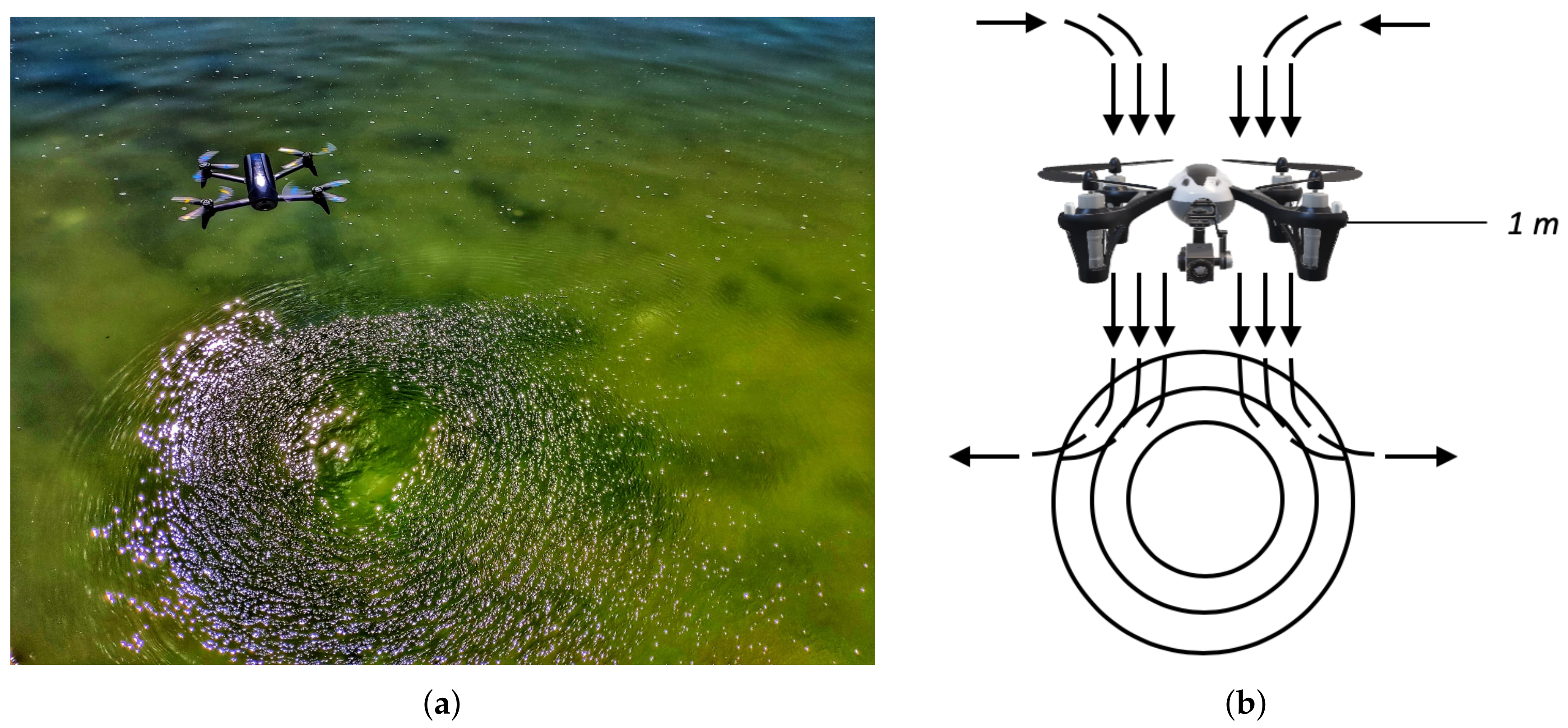
The downwash effect caused by UAV propellers, shown in Figure 1, might have a major impact on terrain classification, because each terrain, when subject to this effect, present different behaviours. Take the example of water-type terrains, where there is no color variation, i.e, no motion presented, these are wrongly classified by algorithms prepared to evaluate static textures, as shown in [2,3,4,5]. This happens because in water it is not possible to observe any texture under these conditions. Using the downwash effect, it adds motion in the environment, and circular textures can be observed, something that normally occurs on water-like terrain.
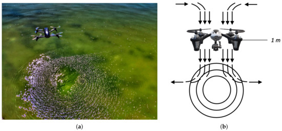
Figure 1.
Downwash Effect: (a) In water terrain; (b) The concept.
Until now, only two recent publications [17,18] were known to use the concept of downwash effect for terrain classification. Ricardo Pombeiro [17] uses the optical flow concept to extract the dynamic part of an image using the Lukas Kanade method [17], from an onboard RGB camera. This work presents a method to determine if the terrain under study was water type or not. However, the algorithm’s extremely long processing time is an issue, since it needs at least four seconds to classify if the terrain under study is water type or not. That means that the UAV needs to stand still for at least four seconds to know which type of terrain it is flying over.
The second most recent work also using the downwash effect to classify terrain types, beyond the use of dynamic properties, also takes advantage of static properties of an image. Unlike in [17], the work presented in [18] not only can identify water, but also sand and vegetation terrains and can do so in near real-time (in less than 30 ms). To classify the terrain type, the system from [18] uses the gabor concept in order to extract the static terrain texture; the optical flow concept, is used under the Farneback algorithm, which obtains the dynamic terrain properties. However, the systems from [17] and [18] only identify one type of terrain per frame, which clearly becomes a disadvantage when there are several types of terrain in a single frame.
The execution of algorithms for terrain classification is computationally heavy and can lead to lower performance than desired. Field Programmable Gate Array (FPGA) implementations have been used to accelerate the execution of algorithms due to their maximization of parallel processing and lower energy consumption [19]. This features allow FPGA implementations to achieve faster execution times when compared to computer vision software libraries, such as OpenCV, or high performance interactive software for numerical computation, such as MATLAB [20,21]. An FPGA-based real-time tree crown detection approach for large-scale satellite images was proposed in [22] and the results showed a speedup of 18.75 times for a satellite image with a size of 12,188 × 12,576 pixels when compared to a 12-core CPU. An ortho-rectification technique based on an FPGA was presented in [23]. Compared to a PC-based platform, to process the same remotely sensed images, the FPGA-based platform was 4.3 times faster. An onboard georeferencing method for remotely sensed imagery was proposed in [24]. The experimental results showed that using FPGA is 8 times faster than using a PC. An FPGA-based method for onboard detection and matching was presented in [25]. The proposed implementation execution speed is 27 times higher when compared to a PC-based implementation. A pattern recognition architecture based on content addressable memory was implemented in [26] and the results show that the worst-case execution time to recognize a pattern is less than a few microseconds. This is 37.12% less then the previous implemented system based on software pattern recognition algorithms [26]. Hardware accelerators, containing content addressable memory and index 8-bit and 16-bit in parallel with each clock cycle, were implemented in [27]. This system consumes as low as 6.76% and 3.28% of energy compared to CPU and GPU-based designs respectively. In the literature, many other articles can be found, such as [28,29,30], describing the usage of FPGAs to support image processing, in real time. The execution times and/or the energy consumption, may justify the use of FPGAs to implement terrain classification and feature extraction algorithms.
This paper proposes a computer vision system that uses static and dynamic features to classify different types of terrain. It uses the downwash effect created by UAV propellers (visible at low altitudes, as shown in Figure 1) to improve the pattern recognition process. The developed system improves the terrain classification accuracy while at the same time, supporting the identification of multiple terrains (water, vegetation, asphalt and sand) in each image. The developed system prototype uses the OpenCV library and it was implemented in a general-purpose computer. It was also partially specified in a Hardware Description Language and implemented in an FPGA based platform.
This paper is organized in seven sections. Section 2 presents the information regarding the UAV used in this paper, whereas Section 2.2 identifies the terrain under study as well as their location. In Section 2.3 we describe the proposed system model of this paper. Section 2.4.1 and Section 2.4.2 contain information about the static texture features, whereas Section 2.5 explains the dynamic extraction to improve the system accuracy to sort terrain. The implementation is described in Section 3. Section 4 shows how the results will be provided using a dynamic map. Section 5 describes and discusses the experimental results, including a comparison with other published results. Conclusions and future work to improve our system are discussed in Section 6 and Section 7, respectively.
2. Experimental Setup
2.1. UAV Platform Design
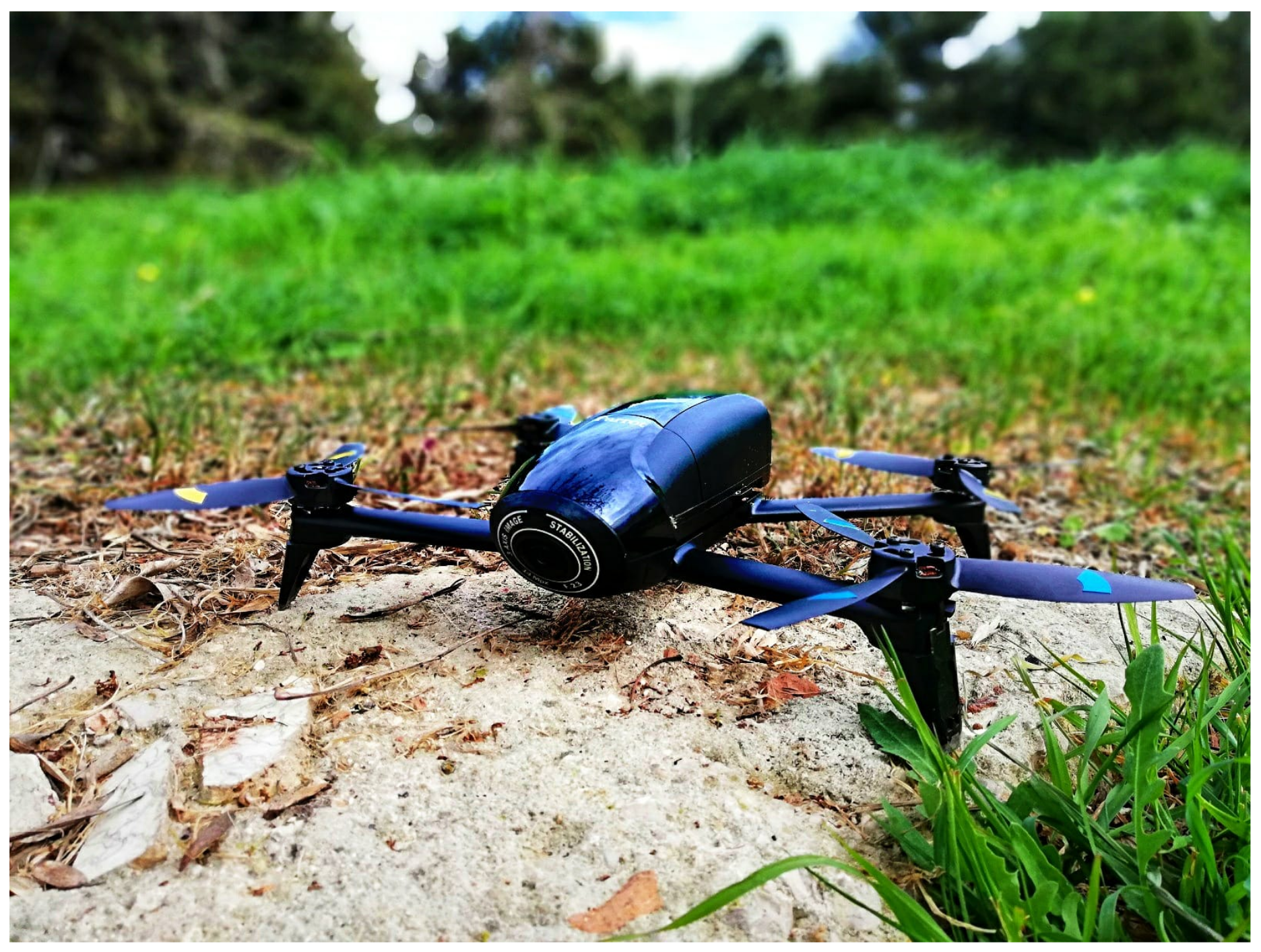
The aerial vehicle used in this work was the Bebop2 [31], a four-rotor UAV from Parrot, shown in Figure 2, with the following characteristics:

Figure 2.
Unmanned Aerial Vehicle - Parrot Bebop2.
- A hardware device to control the low and high level operations. This hardware contains the Global Positioning System (GPS) and the Inertial Measurement Unit (IMU) to detect the UAV position and orientation, respectively. An Wi-Fi receiver is connected to this hardware controller, in order to control UAV motors;
- An RGB camera with a gimbal to stabilize imaging capture. Since the camera technical specifications are known, it is possible to obtain the Field of View (FoV) and therefore, to know the distance (in meters) per pixel. The selected resolution of each frame was 640 × 480 with a rate of 30 Hz;
- A mini controller to stabilize the UAV when it is in flight mode. The sensor used for this purpose was a mini camera pointed to the ground where an optical flow algorithm runs to determine how much the UAV has traveled and to determine the unwanted motion of the UAV and thus reverse the process;
- For autonomous UAV landing, it features a sonar sensor pointed at the ground, in order to detect any obstacle within a six-meter range allowing it to land in an unobstructed zone.
2.2. Data Gathering
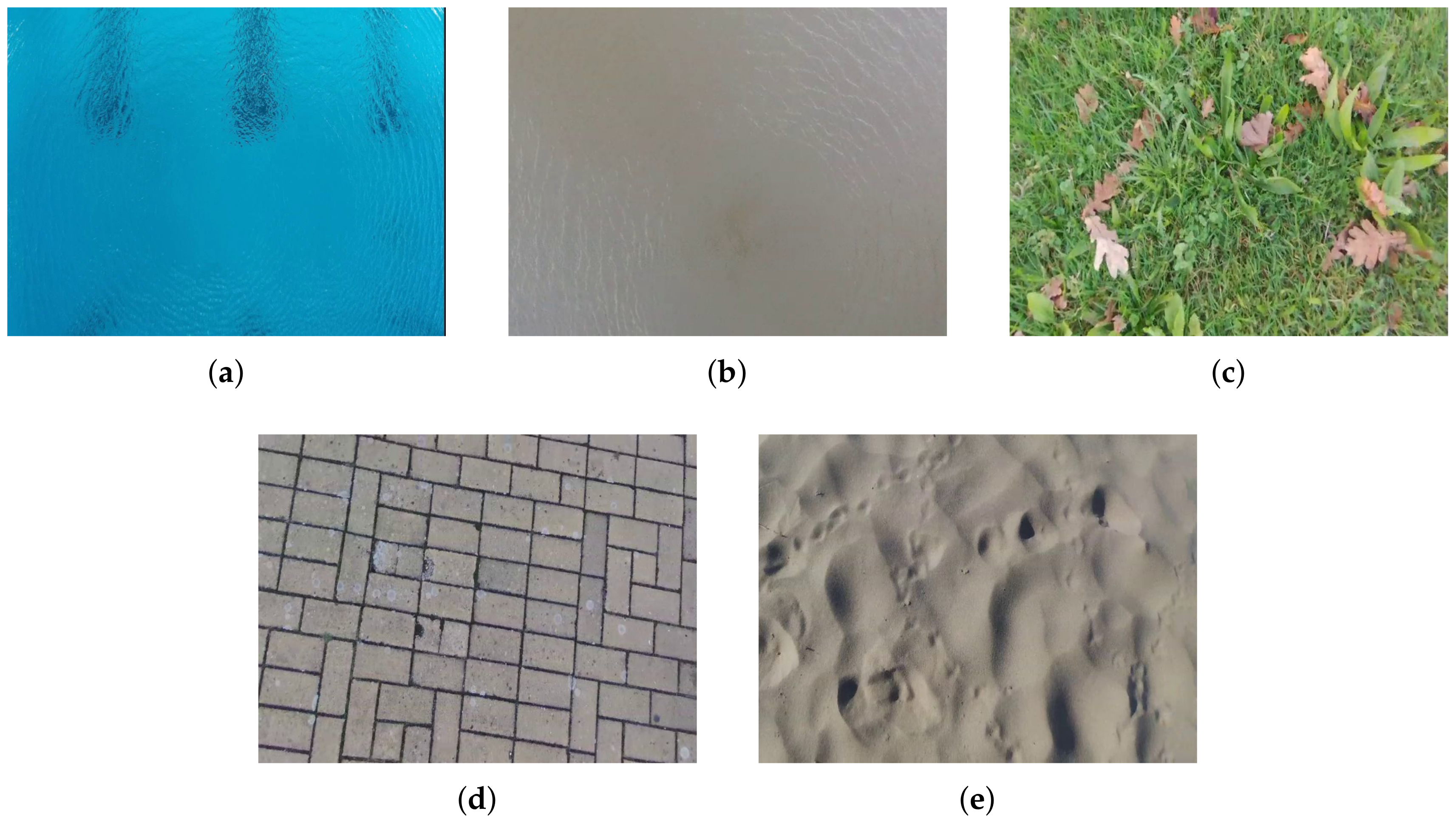
In this paper, four different terrain types (water, vegetation, asphalt and sand) were analyzed, as shown in Figure 3.

Figure 3.
Examples of terrain types: water (a,b); vegetation (c); asphalt (d) and sand (e).
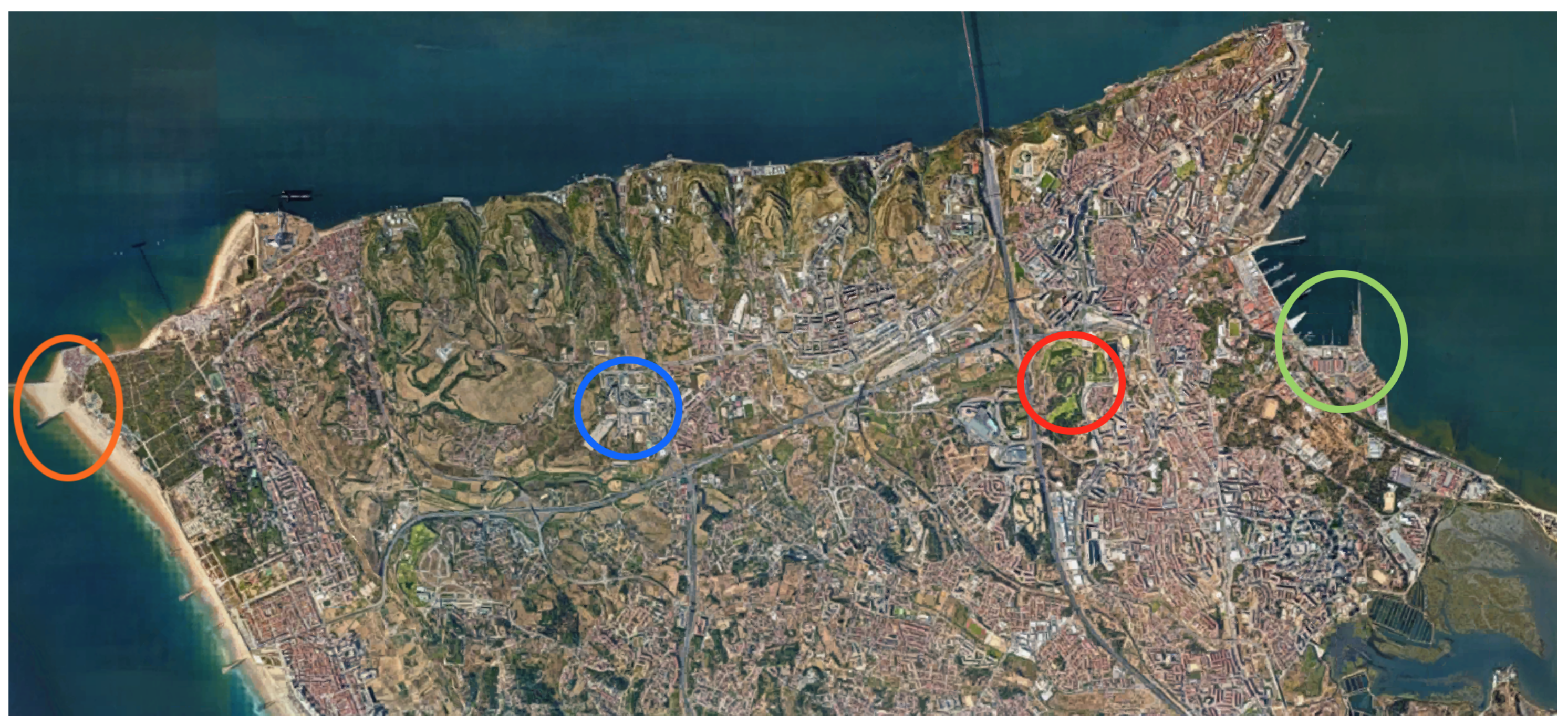
These terrain types were studied at four locations in Portugal as shown in Figure 4:
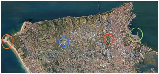
Figure 4.
Data collection localization in Portugal. The circles show the areas where the data set was obtained.
- Orange circle: Costa da Caparica;
- Blue circle: Faculty of Sciences and Technology of NOVA University of Lisbon;
- Red circle: Parque da Paz at Almada;
- Green circle: Portuguese Navy’s Naval Base at Alfeite;
At these locations, it was collected several data in different conditions. Data was collected at an altitude between one and two meters, between 8 a.m. to 6 p.m. Regarding environmental conditions, the authors collected data during both clear and cloudy skies. To avoid overfitting and make the proposed algorithms more robust, older data (with and without the downwash effect) from other locations (e.g., agriculture field at Spain) and from other UAVs (from PDMFC) was also used. Besides, for improving generalization, a technique called “Early Stopping” was used that uses two different data sets: the training set, to update the weights and biases, and the validation set, to stop training when the network begins to overfit the data.
Regarding the cross-validation, this paper used the “k-fold” technique where the data was divided into k randomly chosen subsets of roughly equal size (in this paper k = 5 was chosen).
The complete data set collected is composed by 513.840 images where 161.525 are of water, 95.403 are of vegetation, 31.093 are of asphalt and 225.819 are of sand.
2.3. Proposed System Model
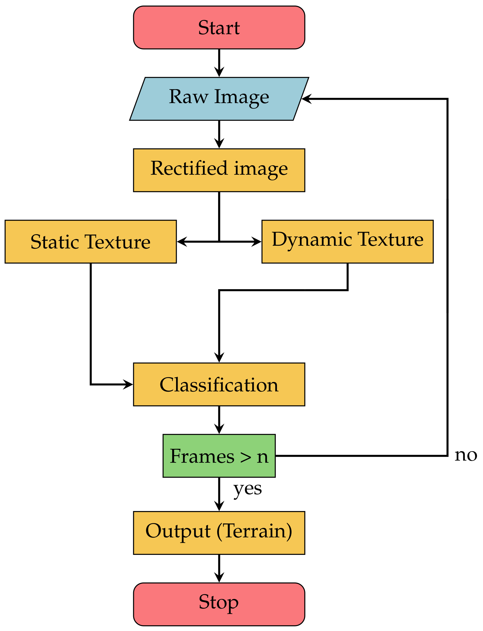
The model of the proposed system, for terrain classification, is presented in Figure 5. As previously mentioned, two main measurements were used in this proposal: Dynamic and Static Textures. Since these two techniques are independent from each other, it is possible to operate it in parallel mode, in order to decrease the time required to process images.

Figure 5.
Proposed system model.
As shown in Figure 5, five main processes were identified in the architecture, namely:
- Rectified Image: It is necessary to calibrate the camera before any process to make the proposed algorithms universal. Only then is possible to work with all RGB cameras regardless of their resolution;
- Static Texture: To extract the terrain’s static textures, Gray-Level Co-Occurrence Matrix (GLCM) and Gray-Level Run Length Matrix (GLRLM) were used to calculate features capable of providing information to classify terrain types;
- Dynamic Texture: To identify the movement of each terrain type, an extraction of dynamic textures was performed using the Optical flow concept;
- Classification: The outputs generated by the static and dynamic extraction phases are turned into inputs for a Neural Network (NN) [32] tasked with classifying the terrain the UAV is flying over. Machine learning techniques have already been proven to be efficient for terrain classification [33,34,35]. In this work, an NN was used, namely a Multilayer Perceptron (MLP) architecture. The Neural Network inputs are the output values from static and dynamic feature extraction algorithms. The Neural Network model consists of three layers: the hidden layer contains 10 neurons, whereas the third layer corresponds to the system output and has four neurons, e.g., four possible outputs (water, vegetation, asphalt and sand). Each neuron uses a sigmoidal function to calculate its output. They are connected as a Fully Connected Feed Forward Neural Network. During the training stage, 70% of the total data was used for training, 15% for testing and 15% for validation;
- Frames > n: “n” is the total number of frames required to increase the algorithm’s accuracy. This threshold value was chosen empirically by the authors.
2.4. Static Textures
Knowing how to take advantage of textures in order to classify any type of terrain is very important for a variety of areas, as already mentioned in Section 1. In this section, we will discuss two types of static texture algorithms: Gray-Level Co-Occurrence Matrix (GLCM); Gray-Level Run Length Matrix (GLRLM).
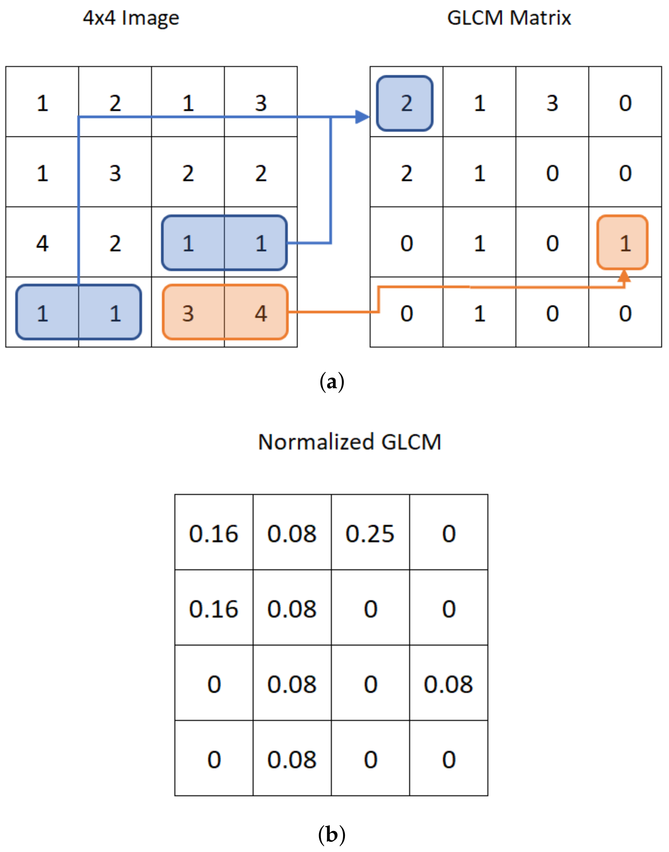
2.4.1. Gray-Level Co-Occurrence Matrix
In this section, it is presented the first static texture algorithm- Gray-Level Co-Occurrence Matrix, known as GLCM [36,37]. This algorithm extracts statistical texture features, that represents textures based on the relation and the distribution between pixels of a given frame. The algorithms that evaluate the texture of a frame can be classified as first, second or higher statistical texture orders. While the first order only calculates properties for individual pixels (such as mean and variance from the original image) neglecting the spatial relationship between pixels, the second and higher texture orders calculate properties of an image using a spatial relationship between two or more pixels, such as GLCM [38,39].
Before building the GLCM of this paper, it is necessary to understand these three parameters:
- The distance d between i and j pixels;
- The angular orientation chosen;
- The Symmetric matrix decision.
After understanding the parameters described above, it is possible to create our matrix for the terrain texture classification.
As a first step, it is necessary to create the GLCM N × N matrix. In this paper the matrix dimensions are 256 × 256 because the input images are defined between 0 and 255 levels (256 gray levels). Figure 6 is an example of a 4 × 4 GLCM matrix. To simplify and make the explanation more intuitive, the following figures will be related to a 4 × 4 GLCM matrix with five gray intensity levels.

Figure 6.
Design of the GLCM matrix from a 4 × 4 image with five gray intensity levels. (a) GLCM matrix with and ; (b) The GLCM normalized matrix.
As it can be seen in Figure 6a, the GLCM matrix was designed to have the distance d, between pixels, equal to 1 with an angular orientation equal to 0 (the distance d and the values were chosen only for the concept description). The GLCM matrix can also be normalized as shown in Figure 6b, by dividing each element by the sum of all image pixels. Lastly, the GLCM can have up to eight different angular orientations (0, 45, 135, 180, 225, 270 and 315 degrees).
After having the GLCM matrix defined, the next step is to determine its transpose in order to become a GLCM symmetric matrix:
In this paper, a , and a symmetric matrix were chosen in order to have a trade-off between noise and system speed. These values were obtained by trial and error.
With a GLCM matrix defined, 6 out of 14 textural features by Haralick [36] were extracted to classify the terrain:
where:
entry in a GLCM normalized matrix as shown in Figure 6b.
- Contrast: Used to return the intensity contrast between a pixel and its neighbor throughout the entire image;
- Correlation: This method is important to define how a pixel is correlated with its neighbor throughout the entire image;
- Energy: Also known as angular second moment, the goal is to evaluate how constant is an image;
- Homogeneity: Know as Inverse Difference Moment, this equation returns 1 when the GLCM is uniform (diagonal matrix);
- Entropy: This feature measures the randomness of intensity distribution. The greater the information’s heterogeneity in an image, the greater the entropy value is. However, when homogeneity increases, the entropy tends to 0;
- Variance: Represents the measure of the dispersion of the values around the mean.
Section 2.4.2 will explain the second static texture algorithm and how to send the feature results to the NN.
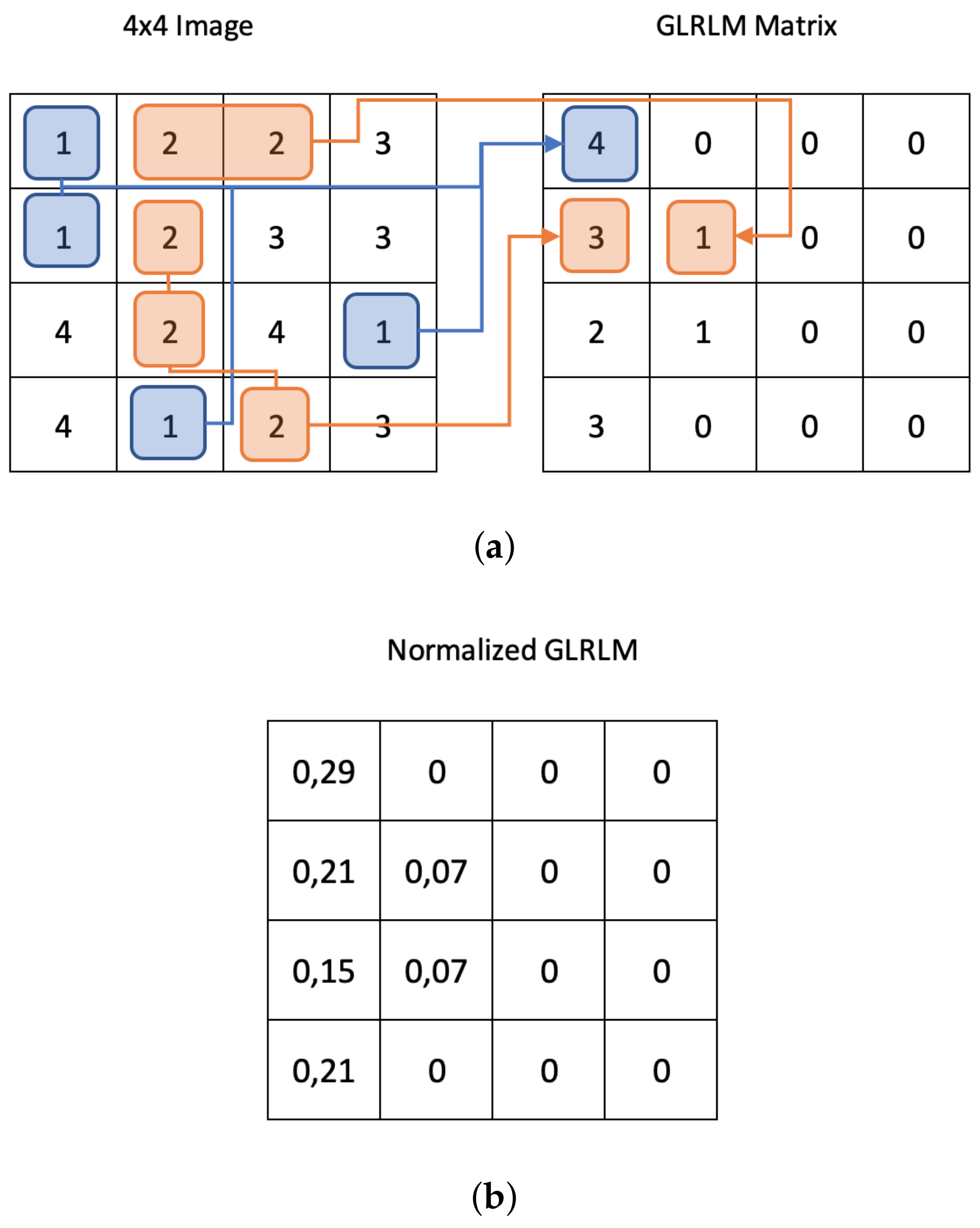
2.4.2. Gray-Level Run Length Matrix
The Gray-Level Run Length Matrix, known as GLRLM, is the second static texture algorithm proposed in this paper. The GLRLM was introduced in [40] to define various texture features. Like the GLCM, GLRLM also evaluates the distribution of gray levels in an image or multiple images. As explained in Section 2.4.1, whereas GLCM evaluates the gray levels within neighbour pixels (taking into account the distance d and the angle ), GLRLM evaluates run lengths. A run length is defined as the length of a consecutive sequence of pixels with the same gray level intensity along direction t.
As with Section 2.4.1, a 4 × 4 matrix (which represents an image of a terrain type) was also created to demonstrate the algorithm. As shown in Figure 7a, the length (columns) of each gray level intensity are calculated for each line. The GLRLM may also have up to eight different angular orientations, t, (0, 45, 135, 180, 225, 270 and 315 degrees).
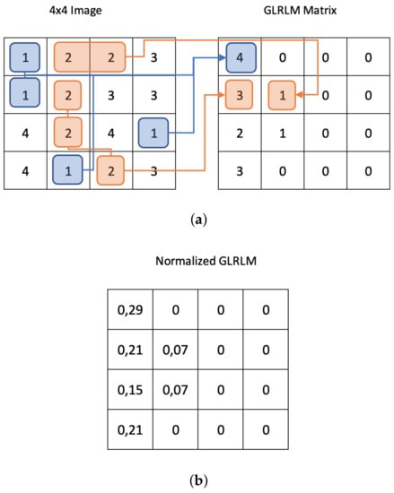
Figure 7.
Design of the GLRLM matrix from a 4 × 4 image with 5 gray levels. (a) GLRLM matrix being ; (b) The GLRLM normalized matrix.
In this work, a 256 × 256 GLRLM matrix with an angular orientation of was used.
After the GLRLM matrix was created, the six features mentioned in Section 2.4.1 are extracted and information is sent to the NN to classify the terrain.
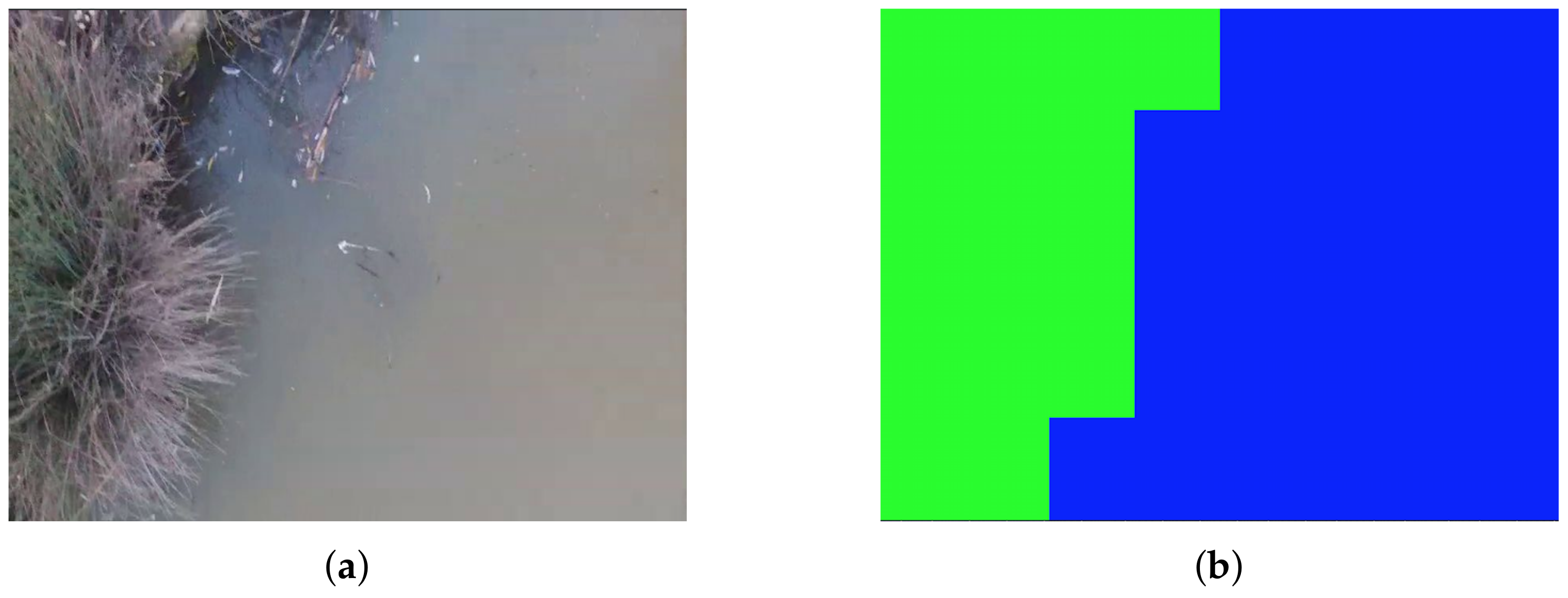
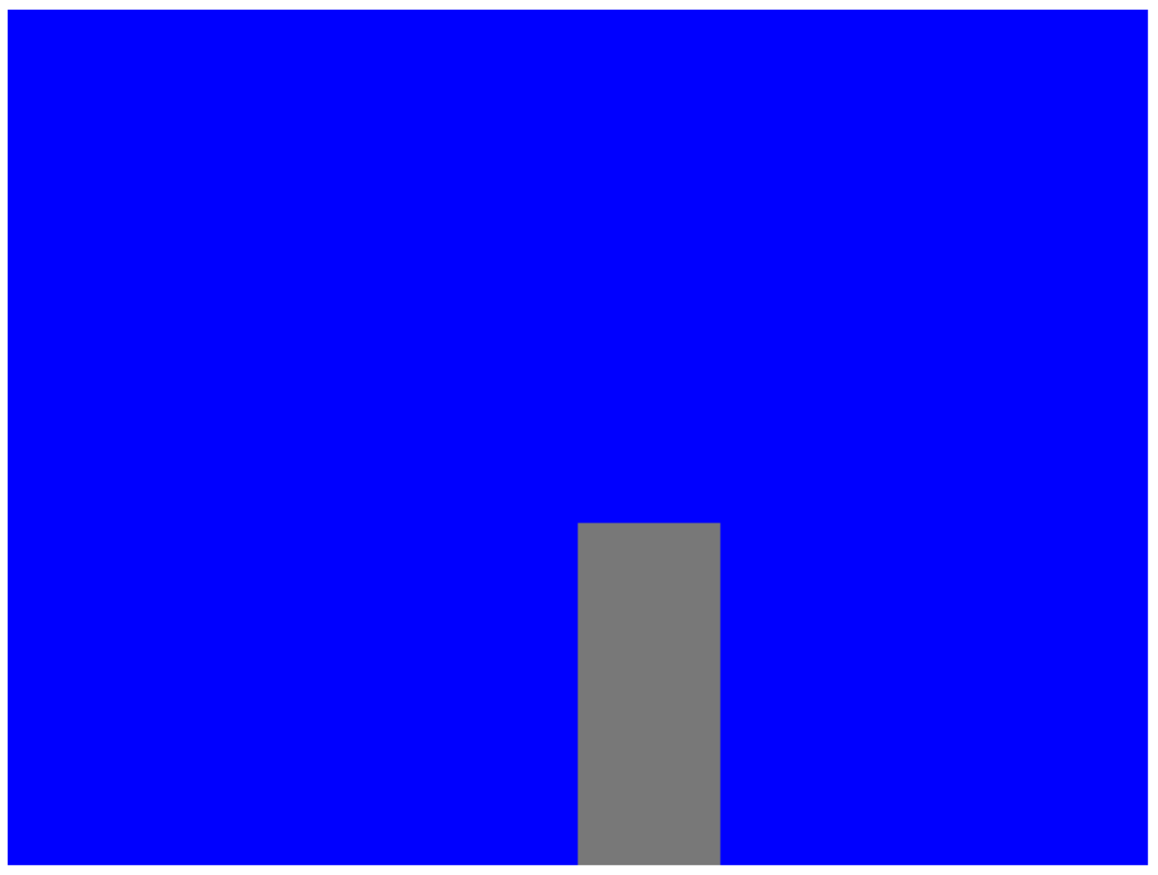
Figure 8 shows an example of an NN response that received information from GLCM and GLRLM, as mentioned in Section 2.4, where the blue area represents water and the green area represents vegetation. For each NN output, a color was used for visualization and validation purposes:

Figure 8.
Neural Network response using static features (GLCM and GLRLM). (a) Two terrains in one frame (vegetation and water); (b) NN results (green is vegetation and blue is water).
- Blue Pixels: Represents water;
- Green Pixels: Represents vegetation;
- Gray Pixels: Represents asphalt;
- Red Pixels: Represents sand.
2.5. Dynamic Textures
The ability to detect static textures for terrain classification is important, as described in Section 2.4.1 and Section 2.4.2. However, the ability to distinguish different terrains using motion analysis increases the accuracy of the system. It is therefore necessary to study several features of different terrains to support the terrain classification.
In this paper the downwash effect from the UAV propellers was studied to extract dynamic textures from water (circular movements), which can be used to differentiate itself from any other type of terrains (vegetation, asphalt and sand).
As mentioned in Section 2.2, different types of terrain create different behaviors when affected by the UAV’s downwash effect. Whereas in water (in this paper lake and pool terrains) it makes a circular pattern, vegetation terrain originates a linear movement and asphalt/sand are almost static. This movement can be detected using a well known concept, namely, Optical Flow.
Optical flow is an image processing method capable of detecting terrain movement in a sequence of frames. There are two well-known algorithms that use the concept of optical flow:
- Lukas Kanade algorithm [41];
- Farneback algorithm [42].
In this work, in order to detect the texture movement, the Farneback algorithm was used [42]. One of the advantages of using the Farneback algorithm is that it provides the flow displacement, , given by the difference in the features between two frames. The flow displacement between features in frame n and can be obtained from Equation (13):
where and are the sample pixels between two consecutive sequence of frames.
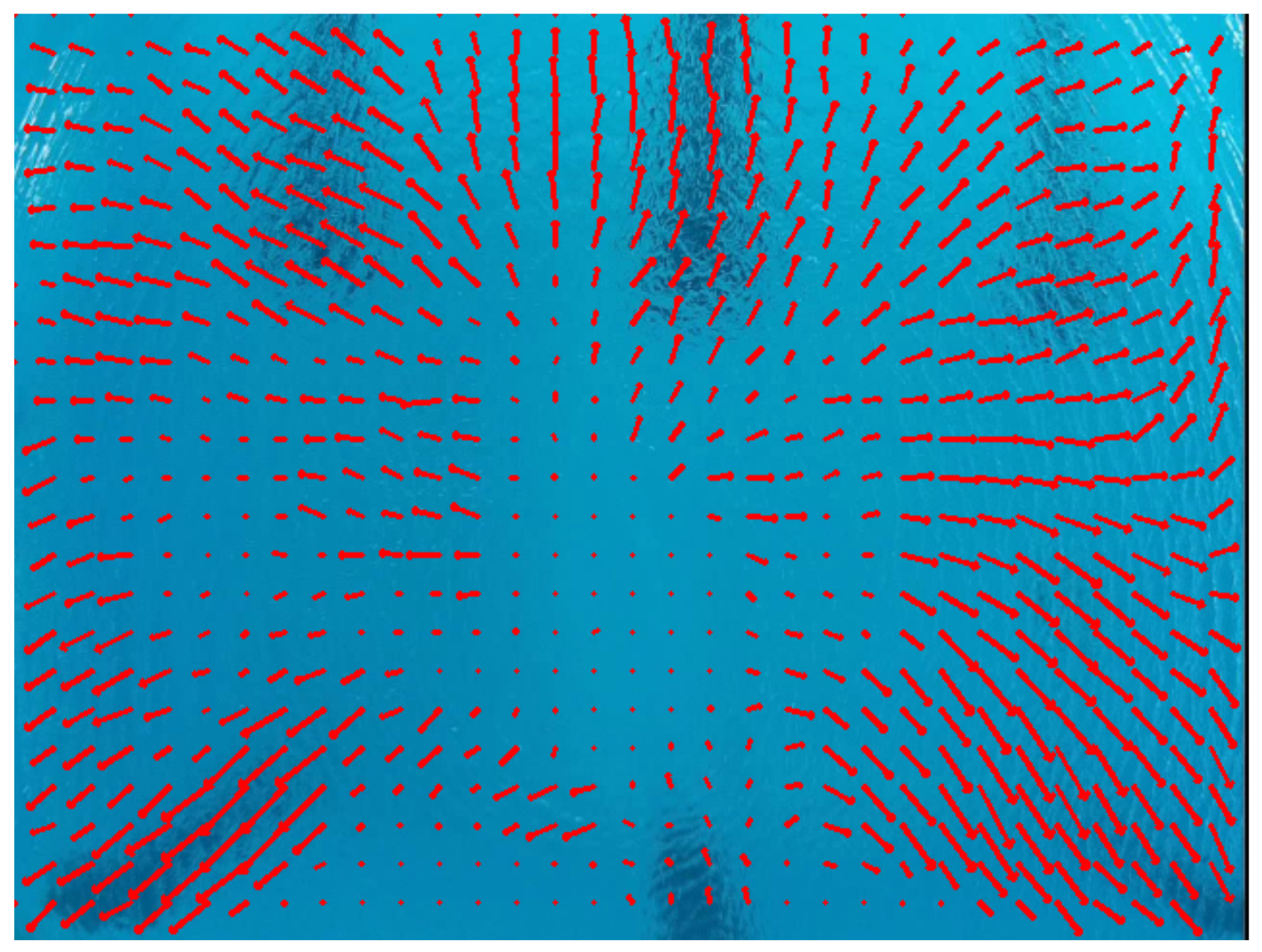
The obtained flows are shown in Figure 9 (red arrows). To determine their density, all linear equations (Figure 10a) were calculated for each flow. In this paper, all line equations are divided by a factor of 20 (this value was obtained by a set of iterations) to make the density of the flows more compact.
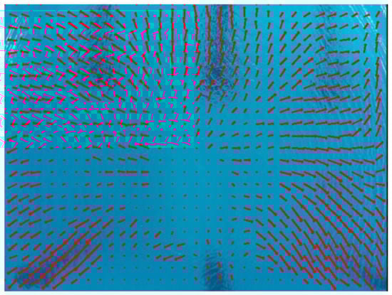
Figure 9.
Example of a Optical Flow concept using Farneback algorithm in water (pool).
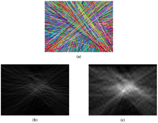
Figure 10.
(a) Linear equations after flow texture extraction; (b) Flow density without dividing by 20; (c) Flow density dividing by 20.
In Figure 10b,c it is possible to observe the difference between a flow density without dividing by 20 and when dividing by 20, respectively.
After the flow density calculation, the next step is to find the maximum value (e.g., the highest pixel value), which is the downwash center. Knowing the center and going back to Figure 9, it is necessary to check, for each flow (arrows in red), whether it is pointing in or out of the downwash center. In this water terrain type example, it is expected that all the flows originated by the Farneback algorithm point out from the center of the downwash (the circular movement goes from the center of the downwash outwards). Thus, there are three possible outputs, when creating a result image:
- Blue Pixels: If the flow is pointing out of the calculated center (downwash center) from the flow density;
- Green Pixels: If the flow is pointing into the calculated center (downwash center) from the flow density;
- Gray Pixels: If the size of the flow is below a certain given treshold.
The result of this example is shown in Figure 11.
Figure 11.
Result of the dynamic algorithm from the concept of optical flow.
Lastly, the output information in Figure 11 is sent to the NN to classify the terrain.
3. Implementation
3.1. Software
This section describes and explains (using pseudo-code) the software implementation (GLCM, GLRLM and Optical Flow) using OpenCV’s libraries and ROS (Robot Operating System) framework:
- Open Source Computer Vision Library (OpenCV): Being an open source library, OpenCV provides a variety of functions used for image processing;
- Robot Operating System (ROS): The Robot Operating System is a “robot application development platform that provides various features such as message passing, distributed computing, code reusing, […]” [43], as well as an integrated software and hardware applied to robotics applications. ROS also provides support for a wide range of programming languages; the possibility of visualizing data (e.g., the content of topics, nodes, packages, coordinate systems graphs and sensor data); and the possibility to write and execute code in a modular way, increasing robustness and also contributing to the standardization of this framework.
The pseudo-code shown in Algorithm 1, describes how the terrain classification system was implemented.
In Algorithm 1, it is possible to identify the main processes of the system represented by the functions: DynamicTexture, StaticTexture, Features and NeuralNetwork. Regarding the gray scale conversion, the system merges the three channels (red, green and blue) using CCIR 601 standard:
Using Equation (14), the dynamic textures (with Optical Flow) and static textures (GLCM and GLRLM) are calculated. The dynamic textures return each pixel flow, as mentioned in Section 2.5. Regarding the static textures, these will return the calculated features from GLCM and GLRLM (i.e., contrast, correlation, energy, homogeneity, entropy and variance) as mentioned in Section 2.4.1 and Section 2.4.2.
The last step is to input these values to the NN and obtain the selected terrain (water, vegetation, asphalt or sand).
| Algorithm 1: Pseudo-Code Software Implementation |
|
3.2. Hardware
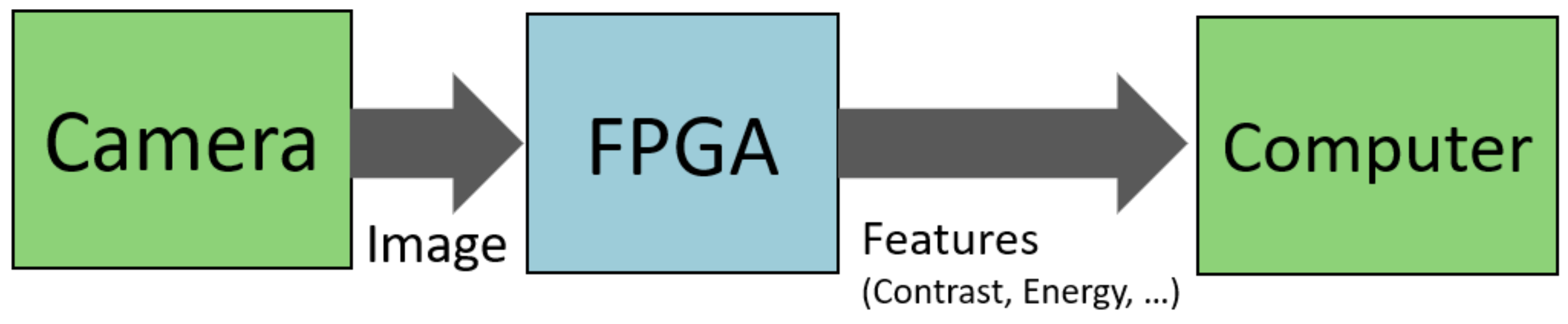
The GLCM algorithm was also partially specified in VHDL (VHSIC Hardware Description Language) code and implemented in hardware, in an FPGA-based platform, which calculates the GLCM matrix and some of image features. This hardware implementation can be integrated with the software implementation as presented in Figure 12. It consists of a camera providing images to an FPGA. The features (contrast, energy) can be determined by applying the GLCM algorithm. The determined features are then sent to the computer, to be processed in software. The implementation of image processing algorithms in hardware can result into smaller execution time, as described in Section 1.
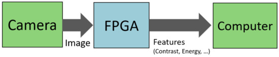
Figure 12.
Hardware integration architecture.
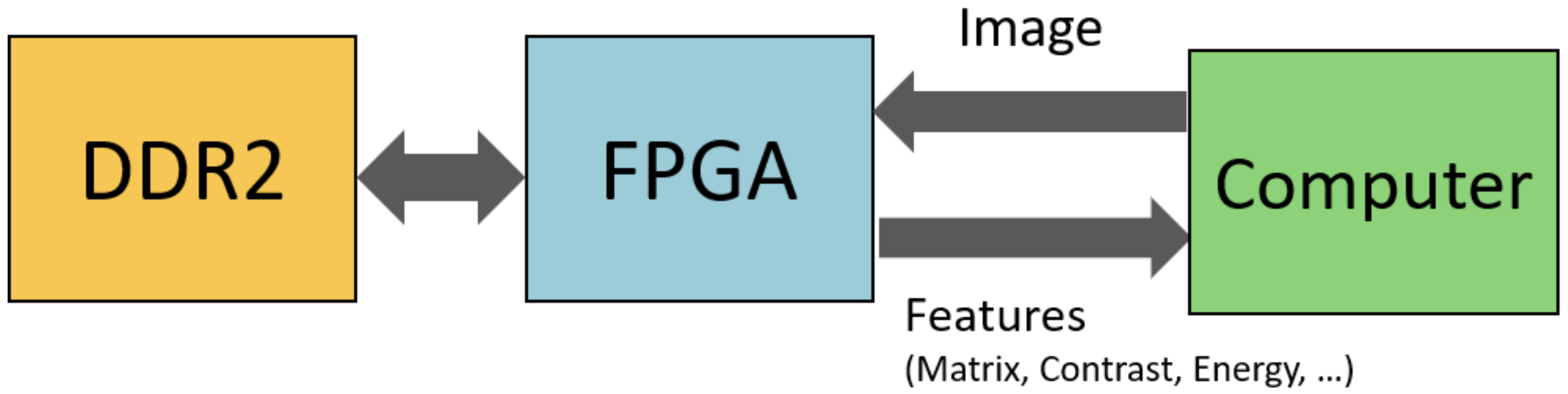
To validate the implemented algorithm, a platform with the architecture presented in Figure 13 was used. It consists of an FPGA, a DDR2 RAM memory and a Computer. The FPGA is used to receive and process the frames, whereas the DDR2 is used to store these frames and the calculated matrices. After processing the images, the FPGA can sends the matrices and their features to the computer. The Avnet Spartan-3A DSP 1800A Video Kit board, which includes a Xilinx Spartan-3A DSP 1800A FPGA and a 128 MB (32 M × 32) DDR2 SDRAM, was used.
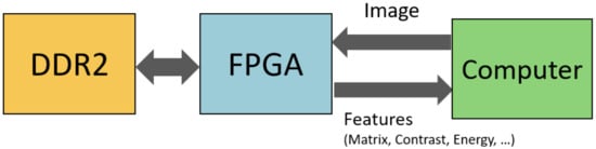
Figure 13.
Validation platform architecture.
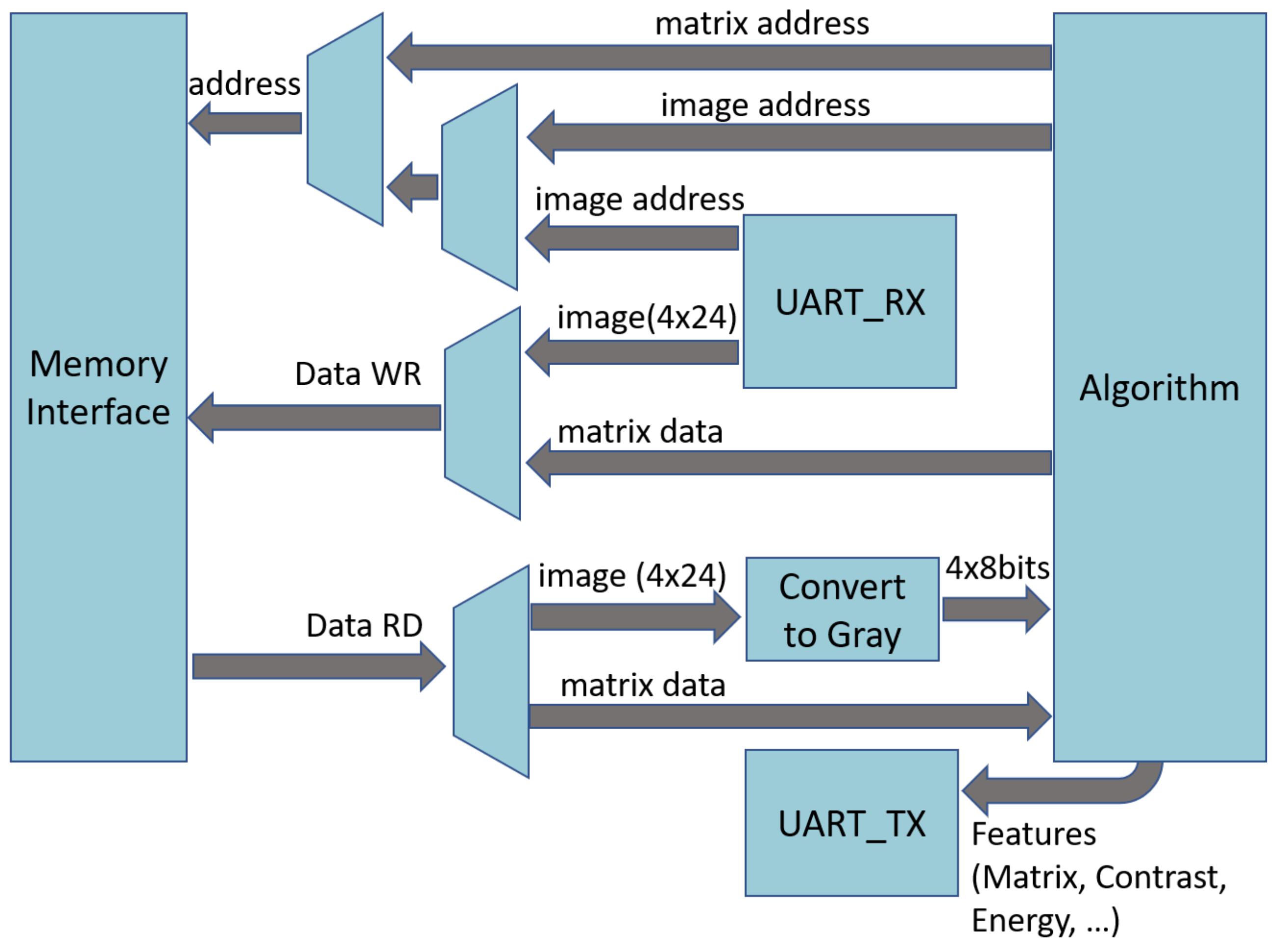
The block diagram, of the hardware prototype implemented in the FPGA, is presented in Figure 14. This block diagram is composed by five main blocks, UART RX, the Memory Interface, the algorithm, the Convert to Gray, and the UART TX. The presented multiplexers and demultiplexers are used to control which addresses are accessed and which data is written or read from the DDR2 memory.
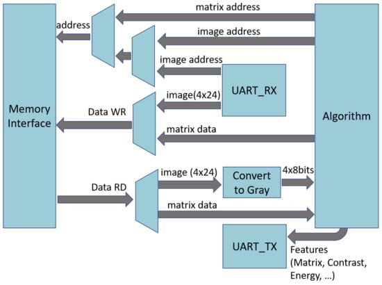
Figure 14.
Simplified Block-diagram/Architecture.
The Memory Interface includes a custom interface that interacts with another interface that was generated using the Core Generator tool available in the Xilinx ISE. It stores and reads the images and their respective features, each in different addresses. The image features are represented by the GLCM matrix, which has a 256 × 256 dimension. The generated DDR2 memory interface has 2 main operations, write and read. The write operation writes data, whereas the read operation returns stored data. These operations can access and give data to the DDR2 in bursts of 4 × 32 bits, which totals 128 bits, or 16 bytes.
The images are transferred from the computer to the FPGA, with the UART RX block being used to accomplish this. It writes pixels with 24 bits each, in the DDR2. When the image is completely stored in the DDR2, the GLCM algorithm can be applied. After the GLCM algorithm executes, the UART TX block sends the GLCM matrices and associated features to the computer.
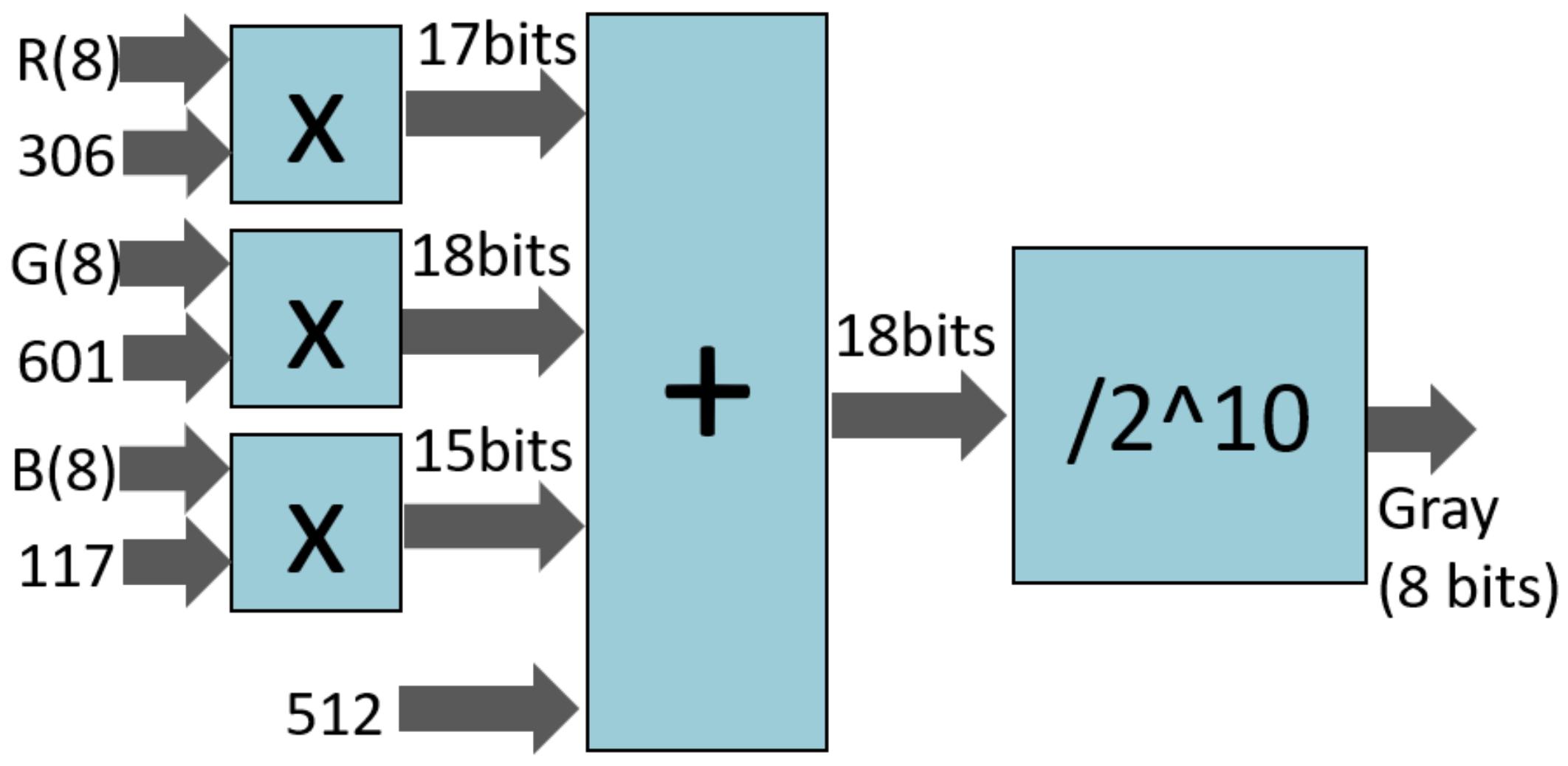
To execute the algorithm, the gray levels of the image must be calculated. The block that performs these calculations is the Convert to gray block, as shown in Figure 15. It receives stored pixels from the DDR2 and applies the grayscale algorithm. The output is the gray level of each pixel, represented by 8 bits (256 different gray levels). The output is used by the algorithm block in order to implement the GLCM algorithm. The implemented grayscale algorithm calculates a weighted average of the Red, Green, and Blue components, using Equation (14). To calculate this, the Red is multiplied by 306 (), the Green is multiplied by 601 (), and the Blue is multiplied by 117 (). Then, the number 512 is added to these three values, to ensure that the final value is properly rounded. Lastly, to obtain the final value, the sum value is shifted to the right 10 bits (divided by 1024 and truncated).
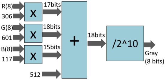
Figure 15.
Convert to gray block diagram.
The Algorithm block diagram, which implements the GLCM algorithm, is displayed in Figure 16. It creates the GLCM matrix, calculates a pair of features, and sends the matrix and the features to the UART TX block. To fill the GLCM matrix with the gray levels, the algorithm block receives, from the convert to gray block, sets of 4 pixels (8 bits per pixel) and saves them in the registers to . For each pair of pixels (), one or two addresses to access the matrix are built with the concatenation of one pixel (, the X in matrix) with the next pixel from the same line (, the Y in matrix). If X is different from Y a second address is built with the concatenation of Y with X. When X is different from Y, for each of the two addresses, the matrix position is read, the value is incremented, and the value is saved. However, if X is equal to Y, only the first address is used, and the value is incremented twice. After processing these four pixels, is saved in , and the next four pixels are received. If the next four pixels are not from the beginning of a line, the pair is also processed. It is important to note that the resulting matrix stored in the DDR2 memory, is already the sum of the matrix with its transpose (Equation (1)), the GLCM symmetric matrix.
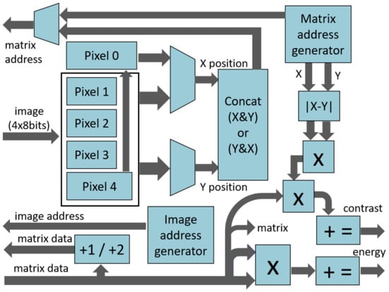
Figure 16.
Algorithm block diagram.
The next step in the algorithm is the calculation of the contrast and energy, which are calculated in parallel. For each position of the matrix:
- the difference between X and Y is multiplied by itself and by the value in the position of the matrix, and the result is accumulated in the contrast register;
- the value in the position of the matrix is multiplied by itself, and the result is accumulated in the energy register.
An FPGA was used to implement the GLCM algorithm in hardware. This device is based on configurable logic blocks, and can be programmed using hardware description languages, such as VHDL (VHSIC Hardware Description Language). The selected FPGA was the Spartan-3A DSP XC3SD1800A, and to program it, the Xilinx ISE 14.7 was used. The VHDL code was synthesized and the circuit implemented. The correspondent device use summary is displayed in Table 1. Only the number of bounded IOBs (pins), DCMs (digital clock managers), and DSP48As (multipliers) surpass 10% of the available resources.

Table 1.
Device use summary.
4. Experimental Design
Aerial Mapping
An aerial vehicle’s autonomy is possible when its route planning and decision making abilities are accurate enough to enable a safe and self-controlled navigation. Furthermore, aerial mapping of the classified terrains using UAVs can be very useful and implemented for many different application kinds such as autonomous navigation, precision agriculture, emergency landings and rescue missions [44].
The fusion between both the techniques applied for terrain classification: static textures (GLCM and GLRLM) and dynamic textures; through MLP, result into several images where each pixel represents one of the four studied terrain types (water, vegetation, asphalt and sand).
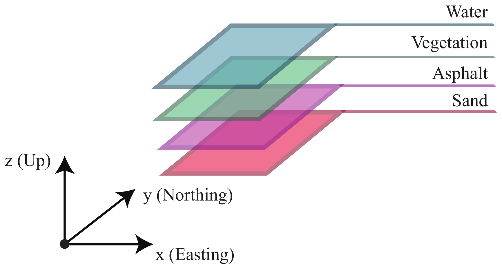
This system’s mapping procedure is similar to the Aerial Semantic Mapping algorithm described for a Precision Agriculture experiment [10]. The framework’s pipeline uses a dynamic ROS grid map composed by four layers (one for each type of terrain, see Figure 17). These layers are converted into the ROS message type which saves a georeferenced map with all the collected and classified images. The layered grid map cells have value 0 (white) when the pixel presents the corresponding layer’s terrain type, otherwise the cell is 1 (black).

Figure 17.
Layered mapping of the classified terrain types.
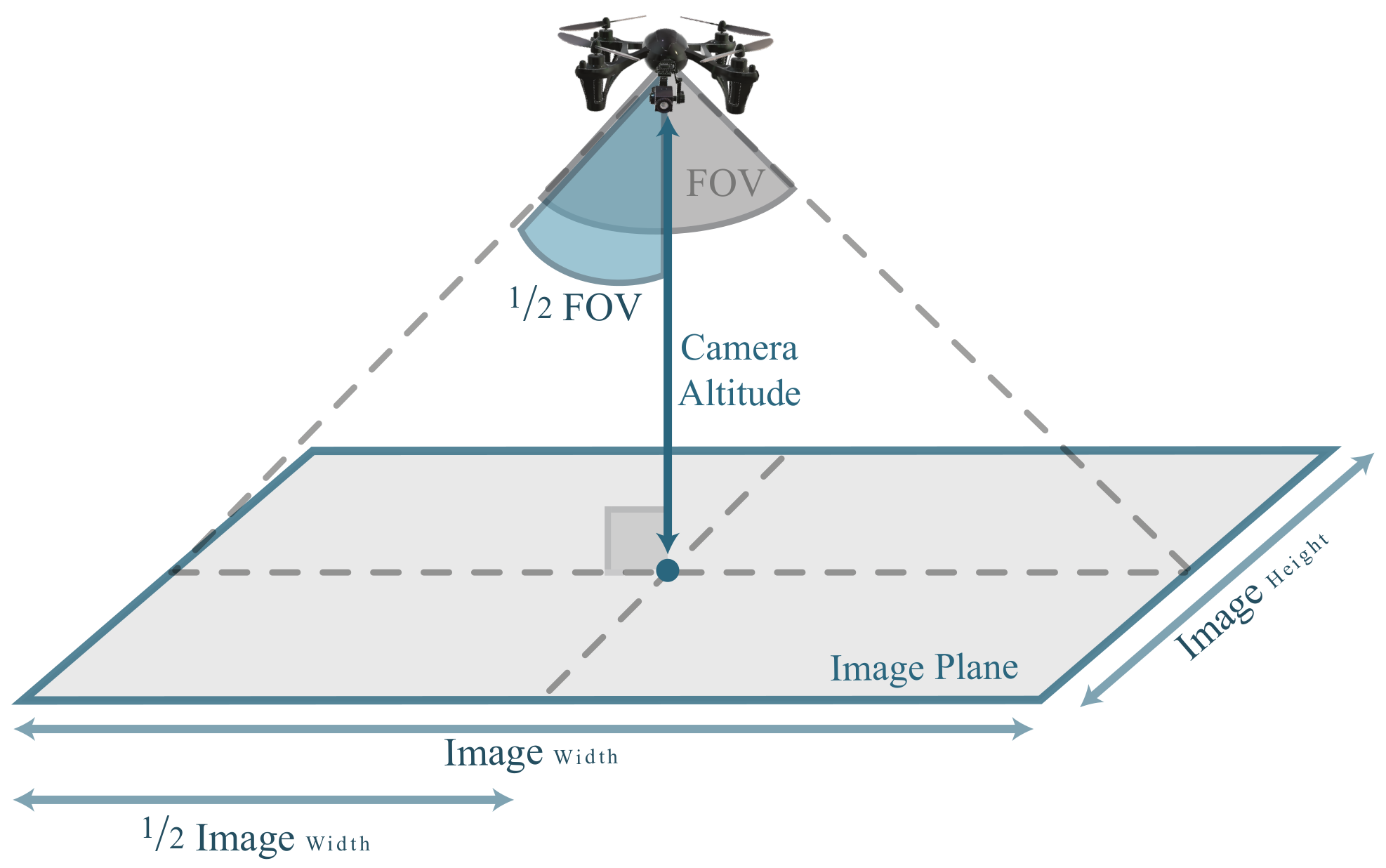
Georeferencing data requires information about GPS coordinates (latitude, longitude and altitude), high precision positioning [45,46], IMU attitude (yaw), camera lense’s FOV, image’s resolution and aspect ratio—Figure 18.

Figure 18.
Schematic of how to determine the real image plane dimension.
Equation (15) computes the real dimensions of the captured area, where FOV is measured in degrees () and the AspectRatio is the image’s height:width proportion factor.
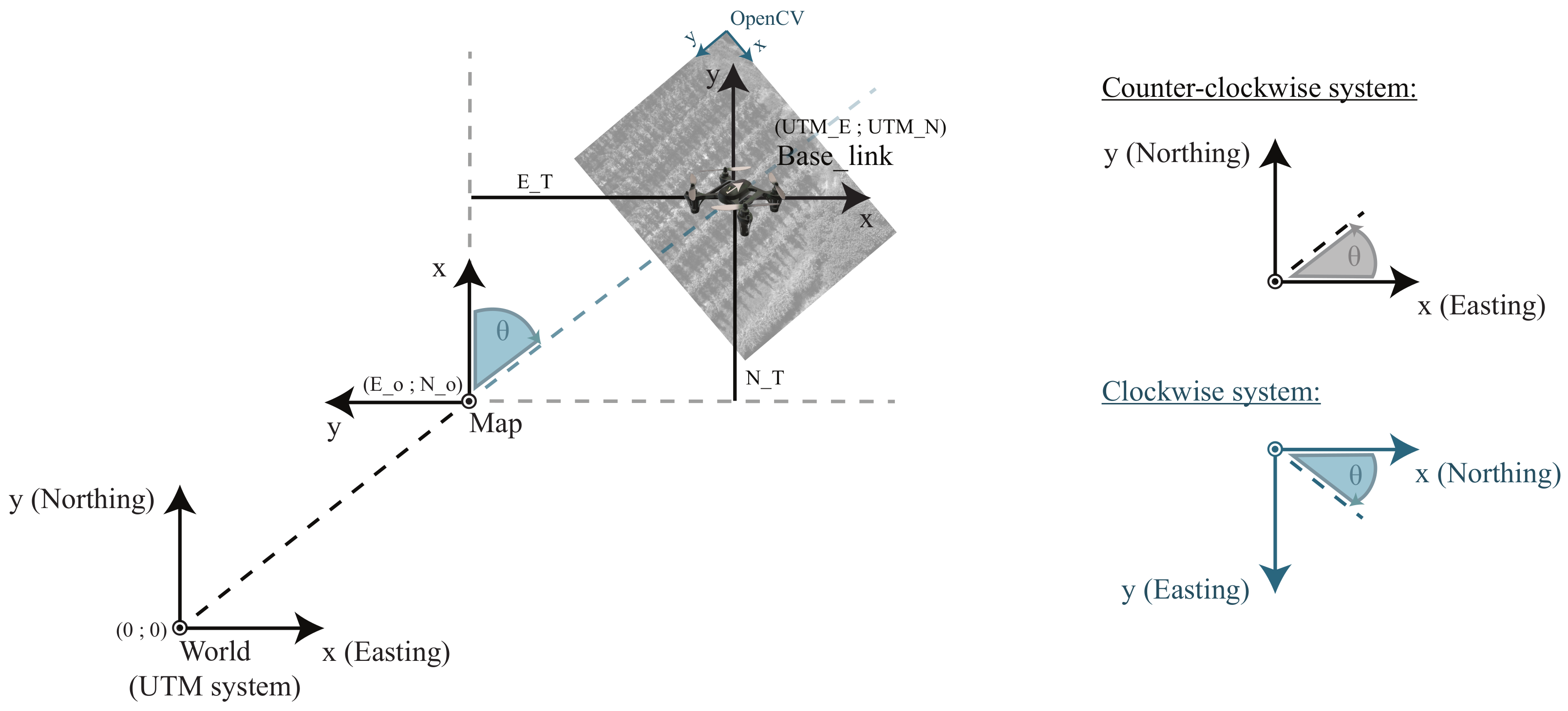
The Parrot Bebop2 (Base_link) uses a counter-clockwise IMU sensor, which is in line with ROS REP:103 conventions [47] followed by the and frames. On the other hand, OpenCV uses a clockwise system, which means that when x-axis points to right, then y-axis is pointing down, Figure 19.

Figure 19.
Interfaces’ coordinate systems: Base_link, world and map (black counter-clockwise coordinate systems), OpenCV (blue clockwise coordinate systems).
The precision implied by computer vision systems and ROS image mapping also requires caution when it comes to implement the proper rotation and translation transformations. As illustrated in the schematic of Figure 19, it is considered the standard 90 counter-clockwise rotation to deal with the world→map transformation in Equation (16).
The following equation determines pixels rotation motion according to a rotation matrix M by (Equation (17)).
Then, according to Figure 19, the first captured image center is positioned at (). The subsequent images will be mapped in line with a pivot rotation, as explained in the following steps, where is the position of each image pixel:
- point translation to map origin ();
- point rotation around the map origin ();
- point back translation to the Base_link origin ();
Equation (18), as explained in [10], describes the pivot rotation applied in mapping procedures, where:
Based on the previous pivot rotation formula, it was possible to successfully compute a dynamic mapping algorithm (Equation (19)) that accurately builds an aerial view over the UAV’s flown area.
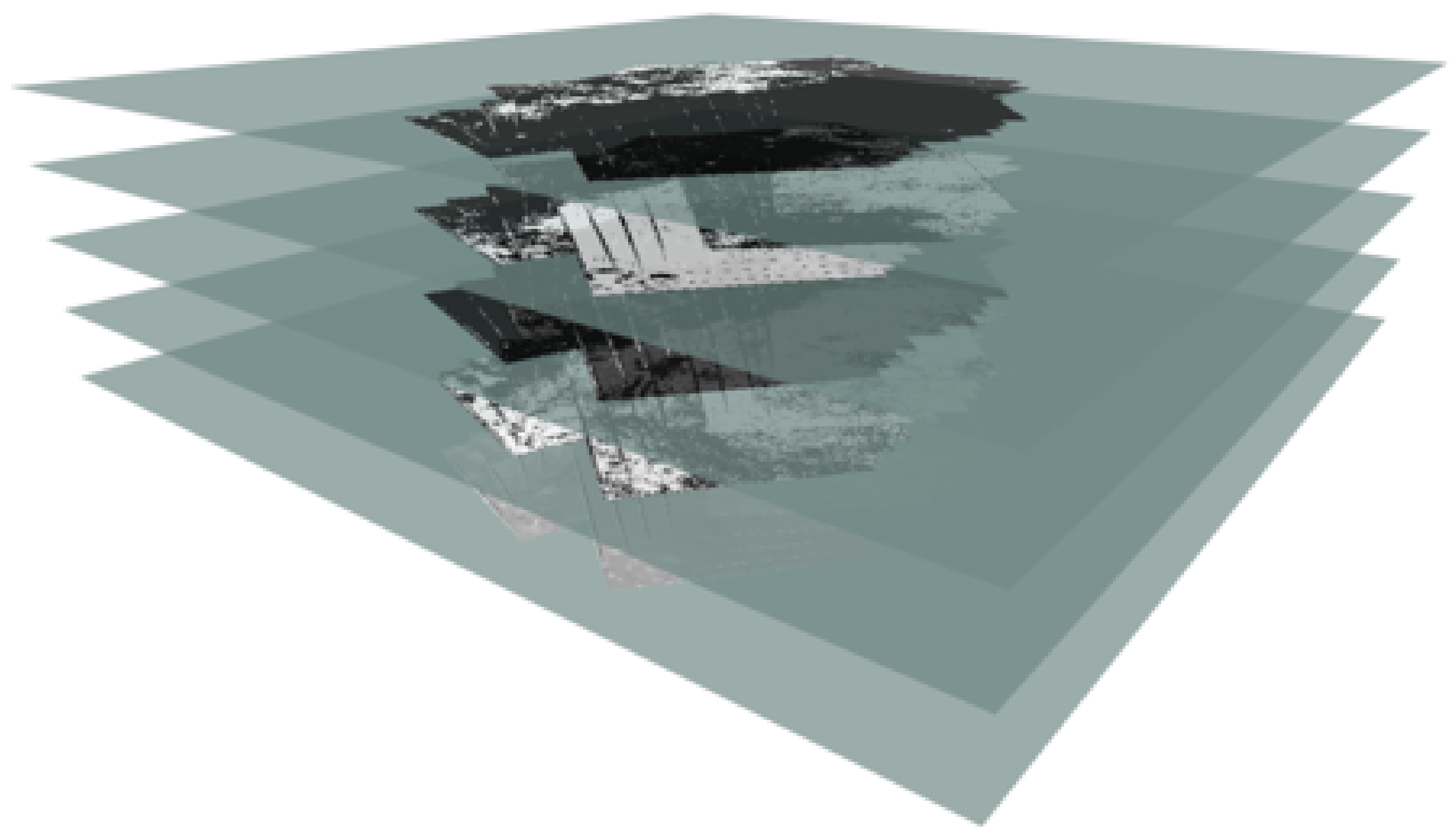
The classified terrain information obtained during this experiment, was all georeferenced and accurately mapped using the ROS grid map layers, as illustrated in Figure 20 and can be visualized using the tool (3D visualization tool for ROS).
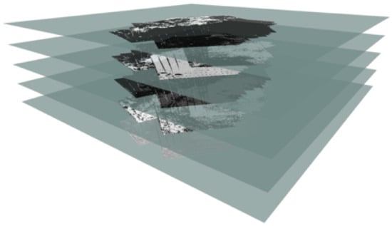
Figure 20.
ROS map result of the four distinct classified terrain types into layers (1st layer- water; 2nd layer- vegetation; 3rd layer- asphalt; 4th layer- sand; 5th layer- images by RGB camera). Georeferenced map visualization using tool.
5. Experimental Results
5.1. Results
The results provided by Section 2.4.1, Section 2.4.2 and Section 2.5, serve as input to the classification algorithm that converts the selected features into output labels. As previously mentioned in Section 2.2, a Multilayer Perceptron (MLP), was used in our experiments. The MLP receives the output values from the static and dynamic algorithms and returns one of four possible terrains (water, vegetation, asphalt or sand).
As mentioned before, the images used in our experiments were taken at an altitude between one to two meters. At lower altitudes the images had poor quality; whereas, above two meters, the downwash effect of the used UAV, which is not a powerful UAV, was almost nonexistent.
The presented results were obtained with a three-layer MLP, with ten neurons on the hidden layer and four neurons for the output layer. Multiple tests were performed with NNs using up to four layers and 100 neurons; however, the differences in the results were insignificant. It is important to mention that this work’s main goal was to identify the best features that can improve the automatic terrain classification system.
In Table 2 it is possible to observe the confusion matrix table, from the classification results using static (GLCM and GLRLM) and dynamic (Optical flow) algorithms. The left column represents the labeled terrain, whereas the for each line, each cell represents the percentage of times the NN identified a certain type of terrain. For example, for the first line, when the terrain is water, the NN succeeds 94.60% in identifying the terrain as water, and fails 5.40% out of the 161.525 considered images. The 5.40% of times it failed, classifies the terrain as follows: 1.88% as vegetation, 1.70% as asphalt and 1.82% as sand.
Table 2.
Results based on GLCM, GLRLM and Optical flow algorithms.
This paper proposals are outlined in Section 5.2, with a comparison between the present work and other approaches. The four terrain types’ classification results are analyzed below.
5.2. Comparison and Discussion of Results
This subsection compares the results obtained by our proposed system, with results obtained by five related works. The comparison is shown in Table 3. For each work we show the respective successful rates for each terrain type as well an overall system average (in the column on the right). The average does not consider always these four terrain types, but each work’s terrain types, since in some of the related works the proposed algorithms do not use all four terrain types. As illustrated in Table 3, the developed system presents the best accuracy in all four terrain types classification: water, vegetation, asphalt, and sand.
Table 3.
Comparison between existing Terrain Classification Systems—Sorted by success rate.
One of the main advantages of this work, when compared to [10,12,16], is the ability to obtain a better classification because the UAV is only 1 to 2 meters away from the ground. In [10,12,16], there are images taken by satellites or at a distance above 60 meters from the ground, which increases the error in the classification of the studied terrain types. In [8,18], the UAV was also used at a short distance from the ground, as in this article, also providing images in high resolution. However, ref. [8,18] only classify one terrain which clearly becomes a disadvantage when there may be several terrain types to be captured by the on-board camera. This work’s developed system has the ability to classify different terrain types in the same image.
Another major advantage studied in the current work, when it comes to terrain classification, is the terrain’s dynamic part usage. This action clearly shows an improved system accuracy, since each terrain behaves differently when affected by the UAV’s downwash effect. According to the works cited in Table 3, only [18] used the dynamic terrain feature, observing that the proposed system’s accuracy is greater than in [8,10,12,16] articles and enhancing the terrains dynamism when it comes to terrain classification. Compared to [18], this work implements different static and dynamic algorithms, as well as classifies different terrain types with increased accuracy.
In summary, the system presented in this paper allows a more accurate terrain classification than with the other works mentioned in Table 3. This is due to the usage of both dynamic (from the Optical Flow concept) and static (from the GLCM and GLRLM) parts of the terrain, as previously mentioned, at 1 to 2 meters height from the ground, in order to have images with higher resolution. The current work, as well as [10], have datasets from the same Portuguese region. When compared to [8,18], the current work uses an extended and more heterogeneous dataset. To allow a direct comparison with these two works (those that use images taken at the same height from the ground), the system developed in this work was also tested with the datasets used in [8,18]. The results are presented in Table 4. Compared to the results presented in Table 3, the system had higher success rates, as expected, due to the smaller and more homogeneous datasets.
Table 4.
Comparison between existing Terrain Classification Systems—Sorted by success rate.
6. Conclusions
This paper presents a complete solution for terrain classification, using the downwash effect by the UAV’s rotors. The system implements two static algorithms: Gray-Level Co-Occurrence Matrix; Gray-Level Run Length Matrix; and one dynamic texture algorithm: Optical Flow. Regarding the terrain classification experimental results, the proposed solution achieves a 95.14% average success rate in differentiating among four terrain types (water, vegetation, asphalt and sand).
The developed FPGA-based prototype validates the use of hardware to implement parts of the proposed system. The integration of this hardware prototype into the system substantially reduces the software processing time and accelerate terrain classification. The developed hardware prototype will be extended in the near future to provide additional image features.
The obtained classification accuracy, the ability to classify more than one terrain in the same image, and a dynamic map generation (with the classification results), provide a set of advantages in the area of cooperative autonomous robots with fully autonomous navigation (e.g., an Unmanned Surface Vehicle (USV) needs to know where the water is to be able to navigate and an Unmanned Ground Vehicle (UGV) needs to avoid it).
The developed system had to overcome a major obstacle between software and hardware with UAVs, due to the limited existing work done in this area. A main goal of this paper work was the development of an open source system that merges ROS, OpenCV, and FPGAs, for UAVs. This system will be the basis for further research into cooperative autonomous robots.
7. Future Work
Despite the good results obtained so far, there are several areas in which improvements are foreseen. We plan to further investigate in the near future the following areas:
- Perform a deeper study on changing of the environment colors, to improve the robustness of the algorithm. Environment color variation, regarding to the different time of the day, could influence the results and therefore false positives/negatives. Although the dynamic texture does not suffer much from these changes, due to the fact that the terrain movement is similar, the static texture could be highly affected;
- Since the algorithm was designed for a UAV flying at an altitude between one and two meters, it is likely that at this altitude the UAV may collide with objects in the environment. The authors of this article developed an algorithm [48] to avoid obstacles, from images taken from a depth camera. However, currently it is only working with static objects. An improved version of this algorithm could be used to support the autonomous navigation of the proposed system;
- It is also important to make a deeper study regarding different camera resolutions in order to improve the robustness of the proposed system, however, the system speed may be affected with higher resolutions.
Author Contributions
Conceptualization, J.P.M.-C. and A.M.; Funding acquisition, L.M.C.; Investigation, J.P.M.-C., F.M., A.B.S., T.C., R.C.-R., D.P., J.M.F. and A.M.; Resources, L.M.C.; Software, J.P.M.-C., F.M., A.B.S., T.C., R.C.-R. and D.P.; Supervision, L.M.C., J.M.F. and A.M.; Validation, J.P.M.-C., F.M., A.B.S., T.C., R.C.-R.; Writing—original draft, J.P.M.-C., F.M., A.B.S., T.C. and D.P.; Writing—review & editing, R.C.-R., L.M.C., J.M.F. and A.M.
Funding
This work is supported by the European Regional Development Fund (FEDER), through the Regional Operational Programme of Lisbon (POR LISBOA 2020) and the Competitiveness and Internationalization Operational Programme (COMPETE 2020) of the Portugal 2020 framework [Project 5G with Nr. 024539 (POCI-01-0247-FEDER-024539)]. This project has also received funding from the ECSEL Joint Undertaking (JU) under grant agreement No 783221. The JU receives support from the European Union’s Horizon 2020 research and innovation programme and Austria, Belgium, Czech Republic, Finland, Germany, Greece, Italy, Latvia, Norway, Poland, Portugal, Spain, Sweden.
Acknowledgments
This work was not possible without the support and commitment of PDMFC Research group. This work was also supported by Portuguese Agency “Fundação para a Ciência e a Tecnologia“ (FCT), in the framework of projects PEST (UID/EEA/00066/2019) and IPSTERS (DSAIPA/AI/0100/2018).
Conflicts of Interest
The authors declare no conflict of interest.
References
- Bestaoui Sebbane, Y. Intelligent Autonomy of UAVs: Advanced Missions and Future Use; CRC Press: Boca Raton, FL, USA, 2018. [Google Scholar]
- Linderhed, A. Image Empirical Mode Decomposition: A New Tool For Image Processing. Adv. Adapt. Data Anal. 2009, 1, 265–294. [Google Scholar] [CrossRef]
- Feng, Q.; Liu, J.; Gong, J. UAV Remote sensing for urban vegetation mapping using random forest and texture analysis. Remote Sens. 2015, 7, 1074–1094. [Google Scholar] [CrossRef]
- Khan, Y.N.; Komma, P.; Bohlmann, K.; Zell, A. Grid-based visual terrain classification for outdoor robots using local features. In Proceedings of the IEEE SSCI 2011: Symposium Series on Computational Intelligence—CIVTS 2011: 2011 IEEE Symposium on Computational Intelligence in Vehicles and Transportation, Paris, France, 11–15 April 2011. [Google Scholar]
- Pietikäinen, M.; Hadid, A.; Zhao, G.; Ahonen, T. Computer Vision Using Local Binary Patterns; Computational Imaging and Vision; Springer: London, UK, 2011; Volume 40. [Google Scholar]
- Ebadi, F.; Norouzi, M. Road Terrain detection and Classification algorithm based on the Color Feature extraction. In Proceedings of the 2017 IEEE Artificial Intelligence and Robotics (IRANOPEN), Qazvin, Iran, 9 April 2017; pp. 139–146. [Google Scholar]
- Lin, C.; Ding, Q.; Tu, W.; Huang, J.; Liu, J. Fourier Dense Network to Conduct Plant Classification Using UAV-Based Optical Images. IEEE Access 2019, 7, 17736–17749. [Google Scholar] [CrossRef]
- Matos-Carvalho, J.P.; Mora, A.; Rato, R.T.; Mendonça, R.; Fonseca, J.M. UAV Downwash-Based Terrain Classification Using Wiener-Khinchin and EMD Filters. In Technological Innovation for Industry and Service Systems. DoCEIS 2019. IFIP Advances in Information and Communication Technology; Camarinha-Matos, L., Almeida, R., Oliveira, J., Eds.; Springer: Cham, Switzerland, 2019; Volume 553. [Google Scholar]
- Khan, P.W.; Xu, G.; Latif, M.A.; Abbas, K.; Yasin, A. UAV’s Agricultural Image Segmentation Predicated by Clifford Geometric Algebra. IEEE Access 2019, 7, 38442–38450. [Google Scholar] [CrossRef]
- Salvado, A.B. Aerial Semantic Mapping for Precision Agriculture Using Multispectral Imagery. 2018. Available online: http://hdl.handle.net/10362/59924 (accessed on 1 December 2018).
- He, C.; Liu, X.; Feng, D.; Shi, B.; Luo, B.; Liao, M. Hierarchical terrain classification based on multilayer bayesian network and conditional random field. Remote Sens. 2017, 9, 96. [Google Scholar] [CrossRef]
- Li, W.; Peng, J.; Sun, W. Spatial–Spectral Squeeze-and-Excitation Residual Network for Hyperspectral Image Classification. Remote Sens. 2019, 11, 884. [Google Scholar]
- Yan, W.Y.; Shaker, A.; El-Ashmawy, N. Urban land cover classification using airborne LiDAR data: A review. Remote Sens. Environ. 2015, 158, 295–310. [Google Scholar] [CrossRef]
- Wallace, L.; Lucieer, A.; Malenovsky, Z.; Turner, D.; Vopěnka, P. Assessment of forest structure using two UAV techniques: A comparison of airborne laser scanning and structure from motion (SfM) point clouds. Forests 2016, 7, 62. [Google Scholar] [CrossRef]
- GruszczynSki, W.; Matwij, W.; Cwiakała, P. Comparison of low-altitude UAV photogrammetry with terrestrial laser scanning as data-source methods for terrain covered in low vegetation. ISPRS J. Photogramm. Remote Sens. 2017, 126, 168–179. [Google Scholar] [CrossRef]
- Sofman, B.; Andrew Bagnell, J.; Stentz, A.; Vandapel, N. Terrain Classification from Aerial Data to Support Ground Vehicle Navigation; Tech. Report, CMU-RI-TR-05-39; Robotics Institute, Carnegie Mellon University: Pittsburgh, PA, USA, 2006. [Google Scholar]
- Pombeiro, R.; Mendonca, R.; Rodrigues, P.; Marques, F.; Lourenco, A.; Pinto, E.; Barata, J. Water detection from downwash-induced optical flow for a multirotor UAV. In Proceedings of the IEEE OCEANS 2015 MTS/IEEE, Washington, DC, USA, 19–22 October 2015; pp. 1–6. [Google Scholar]
- Matos-Carvalho, J.P.; Fonseca, J.M.; Mora, A.D. UAV downwash dynamic texture features for terrain classification on autonomous navigation. In Proceedings of the 2018 IEEE Federated Conference on Computer Science and Information Systems, Annals of Computer Science and Information Systems, Poznan, Poland, 9–12 September 2018; pp. 1079–1083. [Google Scholar] [CrossRef]
- Shawahna, A.; Sait, S.M.; El-Maleh, A. FPGA-Based Accelerators of Deep Learning Networks for Learning and Classification: A Review. IEEE Access 2019, 7, 7823–7859. [Google Scholar] [CrossRef]
- Kiran, M.; War, K.M.; Kuan, L.M.; Meng, L.K.; Kin, L.W. Implementing image processing algorithms using ‘Hardware in the loop’ approach for Xilinx FPGA. In Proceedings of the 2008 International Conference on Electronic Design, Penang, Malaysia, 1–3 December 2008; pp. 1–6. [Google Scholar] [CrossRef]
- Tiemerding, T.; Diederichs, C.; Stehno, C.; Fatikow, S. Comparison of different design methodologies of hardware-based image processing for automation in microrobotics. In Proceedings of the 2013 IEEE/ASME International Conference on Advanced Intelligent Mechatronics, Wollongong, Australia, 9–12 July 2013; pp. 565–570. [Google Scholar] [CrossRef]
- Li, W.; He, C.; Fu, H.; Zheng, J.; Dong, R.; Xia, M.; Yu, L.; Luk, W. A Real-Time Tree Crown Detection Approach for Large-Scale Remote Sensing Images on FPGAs. Remote Sens. 2019, 11, 1025. [Google Scholar] [CrossRef]
- Zhou, G.; Zhang, R.; Liu, N.; Huang, J.; Zhou, X. On-Board Ortho-Rectification for Images Based on an FPGA. Remote Sens. 2017, 9, 874. [Google Scholar] [CrossRef]
- Liu, D.; Zhou, G.; Huang, J.; Zhang, R.; Shu, L.; Zhou, X.; Xin, C.S. On-Board Georeferencing Using FPGA-Based Optimized Second-Order Polynomial Equation. Remote Sens. 2019, 11, 124. [Google Scholar] [CrossRef]
- Huang, J.; Zhou, G. On-Board Detection and Matching of Feature Points. Remote Sens. 2017, 9, 601. [Google Scholar] [CrossRef]
- Mujahid, O.; Ullah, Z.; Mahmood, H.; Hafeez, A. Fast Pattern Recognition Through an LBP Driven CAM on FPGA. IEEE Access 2018, 6, 39525–39531. [Google Scholar] [CrossRef]
- Nguyen, X.; Hoang, T.; Nguyen, H.; Inoue, K.; Pham, C. An FPGA-Based Hardware Accelerator for Energy-Efficient Bitmap Index Creation. IEEE Access 2018, 6, 16046–16059. [Google Scholar] [CrossRef]
- Chaple, G.; Daruwala, R.D. Design of Sobel operator based image edge detection algorithm on FPGA. In Proceedings of the 2014 International Conference on Communication and Signal Processing, Melmaruvathur, India, 3–5 April 2014; pp. 788–792. [Google Scholar] [CrossRef]
- Singh, S.; Saini, K.; Saini, R.; Mandal, A.S.; Shekhar, C.; Vohra, A. A novel real-time resource efficient implementation of Sobel operator-based edge detection on FPGA. Int. J. Electron. 2014, 101, 1705–1715. [Google Scholar] [CrossRef]
- Harinarayan, R.; Pannerselvam, R.; Ali, M.M.; Tripathi, D.K. Feature extraction of Digital Aerial Images by FPGA based implementation of edge detection algorithms. In Proceedings of the 2011 International Conference on Emerging Trends in Electrical and Computer Technology, Nagercoil, India, 23–24 March 2011; pp. 631–635. [Google Scholar] [CrossRef]
- Sphinx Guide Book. 2019. Available online: https://developer.parrot.com/docs/sphinx/index.html (accessed on 30 January 2019).
- Specht, D.F. A General Regression Neural Network. IEEE Trans. Neural Netw. 1991. [Google Scholar] [CrossRef]
- Mora, A.; Santos, T.M.A.; Łukasik, S.; Silva, J.M.N.; Falcão, A.J.; Fonseca, J.M.; Ribeiro, R.A. Land Cover Classification from Multispectral Data Using Computational Intelligence Tools: A Comparative Study. Information 2017, 8, 147. [Google Scholar] [CrossRef]
- Heung, B.; Ho, H.C.; Zhang, J.; Knudby, A.; Bulmer, C.E.; Schmidt, M.G. An Overview and Comparison of Machine-Learning Techniques for Classification Purposes in Digital Soil Mapping. Geoderma 2016, 265, 62–77. [Google Scholar] [CrossRef]
- Giusti, A.; Guzzi, J.; Ciresan, D.C.; He, F.; Rodriguez, J.P.; Fontana, F.; Faessler, M.; Forster, C.; Schmidhuber, J.; Di Caro, G.; et al. A Machine Learning Approach to Visual Perception of Forest Trails for Mobile Robots. IEEE Robot. Autom. Lett. 2016, 1, 661–667. [Google Scholar] [CrossRef]
- Haralick, R.M.; Shanmugam, K.; Denstien, I. Textural features for image classification. IEEE Trans. Syst. Man Cybern. 1973, 3, 610–621. [Google Scholar] [CrossRef]
- Kim, I.; Matos-Carvalho, J.P.; Viksnin, I.; Campos, L.M.; Fonseca, J.M.; Mora, A.; Chuprov, S. Use of Particle Swarm Optimization in Terrain Classification based on UAV Downwash. In Proceedings of the 2019 IEEE Congress on Evolutionary Computation (CEC), Wellington, New Zealand, 10–13 June 2019; pp. 604–610. [Google Scholar] [CrossRef]
- Ojala, T.; Pietikaine, M. Texture Classification. Master’s Thesis, Machine Vision and Media Processing Unit, University of Oulu, Oulu, Finland, 2010. [Google Scholar]
- Materka, A.; Strzelecki, M. Texture Analysis Methods—A Review; Technical Report; Institute of Electronics, Technical University of Lodz: Lodz, Poland, 1998. [Google Scholar]
- Galloway, M.M. Texture analysis using gray level run lengths. Comput. Graph. Image Process. 1975, 4, 172–179. [Google Scholar] [CrossRef]
- Bruce, D.L.; Kanade, T. An iterative image registration technique with an application to stereo vision. In Proceedings of the 7th International Joint Conference on Artificial Intelligence (IJCAI ’81), Vancouver, BC, Canada, 24–28 August 1981. [Google Scholar]
- Farneback, G. Two-Frame Motion Estimation Based on Polynomial Expansion. Lect. Notes Comput. Sci. 2003, 2749, 363–370. [Google Scholar] [CrossRef]
- Joseph, L. Mastering ROS for Robotics Programming; Packt Publishing Ltd.: Birmingham, UK, 2015. [Google Scholar]
- Office of the Secretary of Transportation, Federal Aviation Administration, Department of Transportation. Unmanned Aircraft Systems. Available online: https://www.faa.gov/data_research/aviation/aerospace_forecasts/ (accessed on 12 March 2019).
- Pedro, D.; Tomic, S.; Bernardo, L.; Beko, M.; Oliveira, R.; Dinis, R.; Pinto, P. Localization of static remote devices using smartphones. IEEE Veh. Technol. Conf. 2018. [Google Scholar] [CrossRef]
- Pedro, D.; Tomic, S.; Bernardo, L.; Beko, M. Algorithms for estimating the location of remote nodes using smartphones. IEEE Access 2019. [Google Scholar] [CrossRef]
- REP 103—Standard Units of Measure and Coordinate Conventions (ROS.org). Available online: http://www.ros.org/reps/rep-0103.html (accessed on 7 April 2019).
- Matos-Carvalho, J.P.; Pedro, D.; Campos, L.M.; Fonseca, J.M.; Mora, A. Terrain Classification Using W-K Filter and 3D Navigation with Static Collision Avoidance; Intelligent Systems and Applications; Springer: London, UK, 2019; p. 18. [Google Scholar]


© 2019 by the authors. Licensee MDPI, Basel, Switzerland. This article is an open access article distributed under the terms and conditions of the Creative Commons Attribution (CC BY) license (http://creativecommons.org/licenses/by/4.0/).