DE-Net: Deep Encoding Network for Building Extraction from High-Resolution Remote Sensing Imagery

Abstract

Deep convolutional neural networks have promoted significant progress in building extraction from high-resolution remote sensing imagery. Although most of such work focuses on modifying existing image segmentation networks in computer vision, we propose a new network in this paper, Deep Encoding Network (DE-Net), that is designed for the very problem based on many lately introduced techniques in image segmentation. Four modules are used to construct DE-Net: the inception-style downsampling modules combining a striding convolution layer and a max-pooling layer, the encoding modules comprising six linear residual blocks with a scaled exponential linear unit (SELU) activation function, the compressing modules reducing the feature channels, and a densely upsampling module that enables the network to encode spatial information inside feature maps. Thus, DE-Net achieves state-of-the-art performance on the WHU Building Dataset in recall, F1-Score, and intersection over union (IoU) metrics without pre-training. It also outperformed several segmentation networks in our self-built Suzhou Satellite Building Dataset. The experimental results validate the effectiveness of DE-Net on building extraction from aerial imagery and satellite imagery. It also suggests that given enough training data, designing and training a network from scratch may excel fine-tuning models pre-trained on datasets unrelated to building extraction.

1. Introduction

Buildings are fundamental elements of a physical urban environment [1]. Information such as the location, size, and number, of buildings is indispensable for many geographic and social applications, e.g., building thematic mapping [2], land-use mapping [3], urban planning [4], change detection [5], population estimation [6], etc. Such applications require a widely covered range, high accuracy, and regular updates, which makes high-resolution remote sensing (HRRS) imagery the most suitable data source. Building extraction is aimed to classify every pixel into two types: buildings and background. Although HRRS imagery contains abundant building information enough to discriminate separate building blocks, automatic building extraction remains to be a challenging research subject due to the complexity and heterogeneity in HRRS imagery.

Traditional solutions highly depend on the representativeness of hand-crafted features to identify buildings. A variety of features have been explored, such as color [7], texture [8], shape [9], edge [10], shadow [11], and a particular index [12]. However, these features not only demand professional prior knowledge, but also become fragile on account of the change of sensors, imaging conditions, and locations, which greatly undermines their usability. A desirable method is one that effectively generalizes to various unseen situations, and this is where deep convolution neural networks (DCNNs) shine.

DCNNs have been proven to be the most remarkable progress in computer vision in recent decades. The pioneering work was done by LeCun, who proposed a learning mechanism to automatically find the effective parameters to classify handwritten numbers in [13], and also constructed a seven-layer-depth neural network in [14] which was the fundamental archetype of modern DCNNs. With sufficient computing power and large-scale labeled datasets such as ImageNet [15], PASCAL VOC 2012 [16], ADE20K [17], and Cityscapes [18], DCNNs achieved unprecedented accomplishments in image classification [19,20,21,22], image segmentation [23,24,25,26,27], object detection [28,29,30,31,32], and other computer vision applications. As demonstrated in [33], with the increase of the abstraction level, DCNNs learn hierarchical features including low-level features such as edges and contours, and high-level features that represent more semantic information. Compared with traditional algorithms, DCNNs can find the intricate structure in large datasets and optimize the parameters to represent the objects by complex deep features, which makes them robust enough to generalize to new data [34]. AlexNet [19] consists of five convolutional layers and two fully connected layers. Although it seems shallow according to the succeeding hundred-layer-deep networks, it achieved record-breaking results that led the second-place team by almost 10% in ILSVRC-2012 image classification competition, against all traditional machine learning approaches. Thereafter, DCNNs began to attract massive interest in the field of machine learning and computer vision, and the depth increasingly grew. GoogLeNet [20] and VGGNet [21] were the top two players in ILSVRC-2014 image classification competition. GoogLeNet has 22 convolutional layers made of various-sized kernels, while VGGNet has 19 convolutional layers with 3 x 3 kernels. GoogLeNet also presents a dimensionality reduction technique that dramatically reduced the parameter requirements compared with AlexNet and VGGNet. Both networks further improved about 9% accuracy based on AlexNet, proving that the depth of DCNNs matters. Furthermore, He [22] trained a 152-layer-deep ResNet by introducing the residual module and surpassed humans in the ImageNet top five error rate.

With the highly generalizable features learned from ImageNet dataset [35], many DCNNs trained on it were used as the encoder of semantic segmentation networks [23,25,26,27,36,37,38,39]. The fully convolutional network (FCN) architecture was first presented by Long [23] that performed pixel-wise prediction and achieved state-of-the-art accuracy, and since then, it became the mainstream type of DCNNs in semantic segmentation [24,25,26,27]. FCN converts VGG-16 to a segmentation network by pruning its fully connected layers and separately upsampling the feature maps in the last three stages, using bilinear interpolation. The upsampled features are further fused into results of different coarseness. U-Net [24] and SegNet [25] have symmetric encoder–decoder structures. To retain more information in the encoder, U-net concatenates features in the encoder to the corresponding decoder, while SegNet uses a pooling index to upsample the feature maps with more spatial detail. DeepLab [26], employing ResNet-101 as the encoder, also tries to alleviate the spatial detail loss in downsampling; therefore, the atrous convolution was proposed to increase the receptive field without pooling. PSPNet [27], also fine-tuning ResNet-101, hierarchically groups various global average pooling constructed with scenes prior to enlarging the receptive field and better understanding the global scene.

Building extraction can be seen as a variation of semantic segmentation where DCNNs also obtained revolutionary success. Importantly, the occurrence of many open-source building datasets [40,41,42,43] dramatically promoted the application of DCNNs in building extraction. The Massachusetts building dataset, established by Mnih [40] in 2013, consists of 151 aerial image tiles of 1500 × 1500 pixels. Vaihingen and Potsdam datasets [41] are composed of high-resolution orthophotos and the corresponding digital surface models, and are annotated to classify six land-use types, including buildings. The Inria Aerial Image Labeling Dataset [42] provides images with 0.3-m resolution, whose regions include five cities in Europe. The WHU Building Dataset [43] contains 220,000 building samples from 0.075-m resolution images covering a 450 km² area of New Zealand. These datasets provided valuable training data for many pieces of subsequent research [36,37,38,39,40,41,42,43,44,45,46,47,48]. The early attempt of DCNNs in building extraction followed the patch-based approach that the networks were trained to predict a small patch of a larger image using a sliding window [40,44,45]. Fully connected layers [40,44] or global average pooling layers [45] were used as the classifier, and their outputs were reshaped into the size of the target patch. However, as Maggiori suggested in [46], the patch-based framework misuses the fully connected layers by expecting them to classify and upsample pixels in the meantime and learn inappropriate prior knowledge of patch locations, whereas the FCNs do not suffer from such shortcomings and gained better results.

The outstanding transferability of deep features and success of FCNs promoted the development of building extraction in recent years. Shrestha [36] replaced the original activation function, rectified linear unit (ReLU) [49], with exponential linear unit (ELU) [50] in FCN and used conditional random fields to further improve the result. Lu [37] extracted buildings by segmenting the roof outline with richer convolutional features network and addressed the disconnection problem by geometric morphological analysis. Wu [38] modified U-Net to both predict the building roof and the outline where the outline played a regulation role. Zhang [39] proposed Joint-Net, which uses dense atrous convolution blocks to increase the receptive field and classifies both road and buildings just by changing the loss function. Liu [47] used ResNet as the encoder, and designed the spatial residual inception module for decoding to improve the semantic understanding ability by aggregating features in various levels and scales. The advances in network architectures remarkably inspired the researches in building extraction. However, such methods that mainly modify existing FCNs could limit the creation of diverse and innovative networks, and possibly restrict the long-term progress in problems such as remote sensing imagery understanding and building extraction, because convolutional neural networks (CNNs) such as ResNet and FCNs such as SegNet were originally intended to solve different computer vision problems that are not remote sensing related. The datasets they used for training and an actual building extraction dataset are shown in Figure 1. Note that the ImageNet dataset is an image classification dataset that labels the whole image as a class, such as buildings, while the other three are image segmentation datasets annotating every pixel of the target.

The primary objective of machine learning is to design a model that learns from training data and generalizes to new data. Increasing model complexity improves the model capacity, but since the number of parameters grows, the model tends to memorize known data points and therefore cause overfitting unless given lots of data. This is why a simpler model is always preferred if it provides a satisfactory solution in machine learning. Inspired by that, we intended to design an effective network architecture optimized for building extraction from HRRS imagery. The current segmentation networks are good at object discrimination but suffer from unrecoverable spatial information loss due to excessive downsampling, resulting in unclear boundaries and an imprecise shape. We assume that image segmentation is more sensitive to information loss than image classification, because image segmentation is aimed to output the label of every pixel rather than merely classifying the image. Thus, we propose the Deep Encoding Network (DE-Net). It aggregates striding convolution and max-pooling operation to capture more information during downsampling, employs linear residual modules with SELU activation to retain information, and uses densely upsampling convolution (DUC) instead of bilinear interpolation or deconvolution for resolution recovery, which enables DE-Net to encode spatial information in feature maps. DE-Net is trained by dice and binary cross-entropy loss to address the sample imbalance problem in building extraction. The main contributions of this study are:

1. A novel network for building extraction, DE-Net, is proposed. It is optimized for building extraction, and has a simple structure comprising a small number of parameters. DE-Net is aimed to strengthen both information preservation and building discrimination, and achieves the state-of-the-art performance on WHU Building Dataset;

2. On our self-constructed building dataset consisting of GF-2 satellite images of Suzhou, China, where samples are less in number and worse in annotation accuracy compared with the WHU dataset, DE-Net still significantly outperforms SegNet, U-Net, RefineNet [51], and DeepLab v3 + [52];

3. Rich self-comparison experiments are carried out to discuss the effect of modules adopted in DE-Net, concerning the network depth, upsampling method, network width, activation functions, and loss functions. The results provide useful information for future building extraction network architecture innovation.

The rest of this article is organized as follows. In Section 2, the details of the DE-Net are explained. Section 3 presents the experiments on two datasets that demonstrate the advance of DE-Net numerally and visually. In Section 4, we discuss an insight from the experiments and the effect of different modules adopted in DE-Net. Section 5 is the conclusion of this study.

2. Materials and Methods

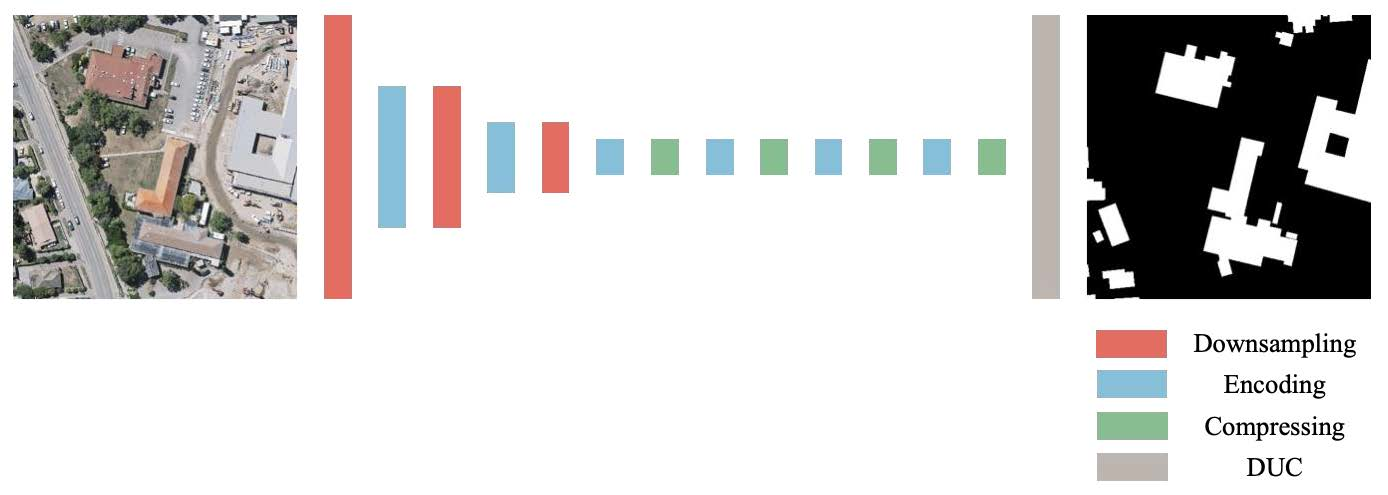
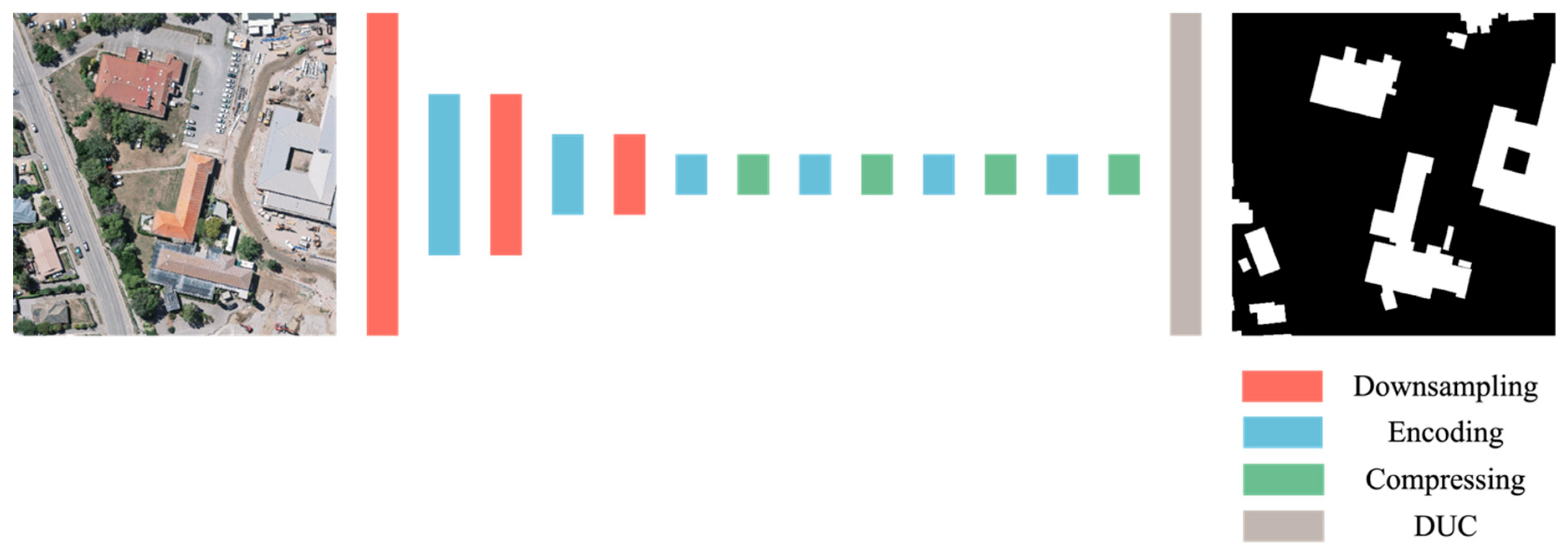
2.1. Architecture Overview

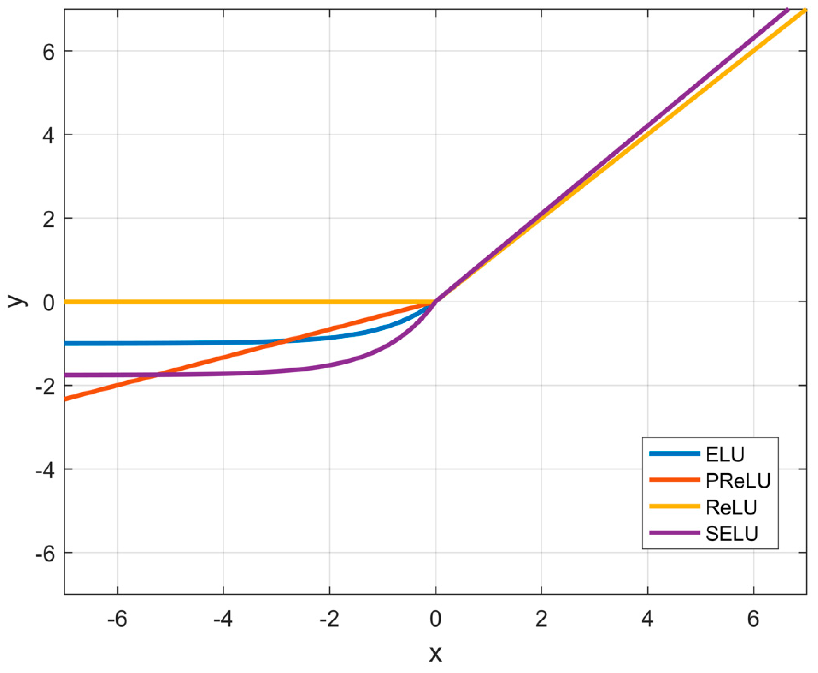
The proposed network, DE-Net, is an end-to-end network that takes high-resolution images as the input and performs building extraction at a pixel scale, as demonstrated in Figure 2. It consists of four different components: the downsampling component, encoding component, compressing component, and DUC component. In common practice, downsampling is usually implemented by a single pooling layer. Here, we followed the idea of Inception that downsamples the input by a striding convolutional layer and a max-pooling layer, and concatenates the two outputs, both downscaling the input by a factor of two. After each downsampling module is an encoding module comprising of six linear residual modules which use scaled exponential linear unit (SELU) [53] in place of ReLU for activation. While the downsampling module expands the feature maps, the compressing module reduces them in the second half of the network, which is also followed by an encoding module. For resolution recovery, DE-Net applies densely upsampling convolution (DUC) to obtain the final high-resolution pixel-wise prediction map. The reason and implementation details of each module are described in the following sections.

2.2. SELU

Since we intend to strengthen the information preservation, a modification can be realized on the indispensable non-linear activation layers. The traditional activation function choice is ReLU function, as expressed in Equation (1). It introduces non-linearity to the network and is also easy to compute the gradient for its simple structure. However, by zeroing out all non-positive data, it generates dead neurons and loses valuable information during activation. Hence, many researchers have proposed alternative activation functions such as parametric rectified linear unit (PReLU) [54], ELU, and SELU, which all map the non-zero input to non-zero output to solve the problem, as shown in following expressions and Figure 3:

$$ReLU\left(x\right)=\{\begin{array}{ll}x& ifx>0\\ 0& ifx\le 0\end{array}$$

(1)

$$PReLU\left(x\right)=\{\begin{array}{ll}x& ifx>0\\ \alpha x& ifx\le 0\end{array}$$

(2)

where $\alpha$ is a learnable parameter:

$$ELU\left(x\right)=\{\begin{array}{ll}x& ifx>0\\ \alpha e^x-\alpha & ifx\le 0\end{array}$$

(3)

where $\alpha$ is not learnable and equals 1 by default:

$$SELU\left(x\right)=\lambda \{\begin{array}{ll}x& ifx>0\\ \alpha e^x-\alpha & ifx\le 0\end{array}$$

(4)

where $\alpha =1.673$ and $\lambda =1.051$, as given in [53].

DE-Net is designed to avoid such deficiency by replacing ReLU by SELU. SELU is originally designed to realize self-normalization in feed-forward neural networks (FNNs). Intuitively, by producing both positive and negative output, it shifts the mean value of layers, and the lambda parameter makes the gradient larger than 1 so that the internal variance of the layers can be scaled in the meantime. A detailed explanation would be out of the scope of this paper. Although SELU provides an alternative way to implement normalization to batch normalization (BN), in our experiments, we find that combining SELU and BN in encoding modules outputs the best results. It’s worth mentioning that SELU only appears in encoding modules, the downsampling modules and compressing modules use ReLU and BN instead, which is discussed in Section 2.3.

2.3. Modules

ResNet changes the scheme of very deep CNNs as it connects the input and the output of residual blocks by addition, pushing the network to learn residual features, and achieves unprecedented success. However, in [55], Sandler pointed out a potential place to be improved: the last ReLU activation function. It is proved that the only scenario that ReLU transformation can save complete information about the input manifold is when the input manifold can be embedded into a low-dimensional subspace of the input space, which indicates that using a linear layer instead of a ReLU activation layer benefits information preservation and therefore promotes the performance. The linear residual block was proposed to realize such an effect. In practice, to make a residual block linear, simply remove the non-linear activation in the end. A linear residual block is shown in Figure 4a. To train a deep network that exploits multi-level features and prevents it from suffering undesirable information loss, an encoding module in DE-Net is made up of six linear residual blocks. As stated in Section 2.2, ReLU is replaced with SELU in all linear residual blocks for the same reason.

The input of an encoding module comes from a downsampling module or a compressing module, which are responsible for reducing the spatial resolution or channel dimension respectively, shown in Figure 4b,c. Similar to how Inception implements downsampling, our downsampling modules combine a convolutional layer with a stride of two and a max-pooling layer to take advantages of these two complementary downsampling methods. The compressing module resembles a linear residual block except that it does not expand the channel dimension in the last convolutional layer, and its output has no connection to its input to learn residual features. In both modules, the information loss is expected to play a beneficial role so that the ReLU activation function is implemented.

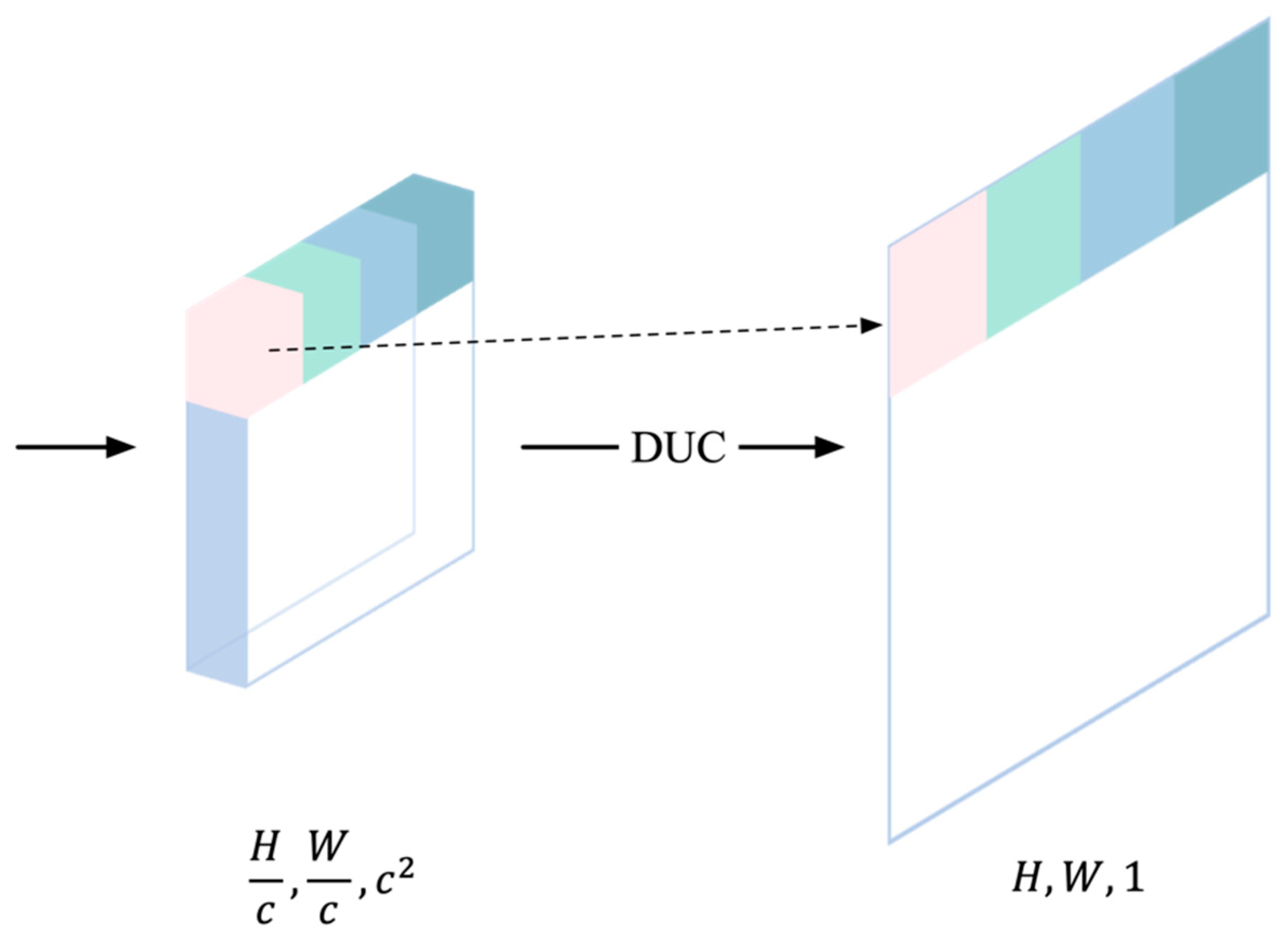
2.4. Densely Upsampling Convolution Module

An inevitable problem of current segmentation networks is the spatial information loss during downsampling. Researchers proposed various ways to alleviate it, such as indexed max-unpooling in SegNet, feature concatenation in U-Net, and atrous convolution in DeepLab. Such techniques significantly contributed to the success of FCNs in image segmentation. In detail, FCNs typically have an encoder–decoder architecture, and the essence of these techniques is to pass the spatial information in the encoder to the decoder, such as in SegNet or U-Net, or to decrease the necessary downsampling steps in the encoder, such as in DeepLab. The decoder is responsible for recovering spatial resolution and generating the segmentation result, given the features learned by the encoder. However, no matter how the encoder tries to save the spatial information, the spatial detail surely loses during downsampling, and once the downsampling rate surpasses an object’s length, the object may not be recovered by the decoder. U-Net and DeepLab may be less affected because U-Net connects every stage of its encoder to its decoder, and DeepLab has a lower downsampling rate. The way they upsample the feature maps is either not learnable, bilinear interpolation, or has unnecessary zero insertion, deconvolution, which means the prediction takes place in downsampled data.

The spatial information plays a key role in building extraction, as it heavily influences the building detail. Besides the efforts mentioned previously, we followed the idea of densely upsampling convolution (DUC) [56] to realize pixel-wise prediction. DUC has no actual upsampling layers; instead, it reshapes the output feature map from $\frac{H}{c}\times \frac{W}{c}\times c^2$ to $H\times W\times 1$ where H, W, c² are the input height, input width, and output channel number, as shown in Figure 5. With the DUC module, the network no longer needs traditional upsampling layers for decoding to recover the input spatial resolution, because it encodes the complete spatial information in all feature maps by convolution, and the final prediction is therefore pixel-wise.

2.5. Dice and Binary Cross-Entropy Loss

Loss functions set the rules to evaluate the distance between network prediction and ground truth. Different loss functions have different emphasis, driving the network to learn differently given the same pair of input data and ground truth. Even a well-designed network may be hindered by a thoughtlessly selected loss function. For our study case, building extraction can be seen as a binary segmentation problem where the binary cross-entropy (BCE) loss function is most commonly used, as given by Equation (5). However, satellite building images have an imbalance problem between building pixels and background pixels, where the BCE loss function is prone to get trapped in local minima, and the network tends to predict the background for a good loss value and fails to learn representative features of the minor class. One way to address this problem is to put a prior weight on each class when computing loss—a bigger weight for buildings in this case—which introduces additional hyper-parameters that need careful tuning. Another way is to choose a less biased function, such as what we used, dice and BCE loss.

Dice and BCE loss integrates dice loss and BCE loss by addition to combine the advantages of both functions. BCE loss function well expresses the misclassification and is easy to compute the gradient mathematically despite the aforementioned defect. The dice loss function, as given by Equation (6), is built on a dice coefficient that evaluates the overlap between the prediction and the ground truth. The more they match, the closer dice coefficient is to 1, pushing the dice loss to 0. However, even when the prediction is completely wrong, the largest loss value that the dice loss function can generate is 1. This is where the BCE loss function performs ideally, as the logistic function in the BCE loss function can generate values much larger than 1, which accelerates the optimization progress. The dice and BCE loss is given by Equation (7):

$$L_1=-{\displaystyle \sum }_{n=1}^N{y}_n^{\prime }\log y_n+\left(1-y_n^{\prime }\right)\log y_n$$

(5)

$$L_2=1-\frac{2{{\displaystyle \sum }}_{n=1}^N{p}_n\times t_n}{{{\displaystyle \sum }}_{n=1}^N{p}_n+{{\displaystyle \sum }}_{n=1}^N{t}_n}$$

(6)

$$L_3=L_1+L_2$$

(7)

where $N$ is the pixel number, $n$ is the pixel index, $y\prime$ is the pixel label class, $y$ is the predicted probability of the pixel being the positive class, $p$ is the predicted pixel class, and $t$ is the true pixel class. In this study, the building pixels are the positive class, and the background pixels are the negative class.

2.6. Evaluation Metrics

Four metrics are used for quantitative evaluation. They are precision, recall, F1-Score, and intersection over union (IoU):

$$Precision=\frac{TP}{TP+FP}$$

(8)

$$Recall=\frac{TP}{TP+FN}$$

(9)

$$F_1=2\times \frac{Precision\times Recall}{Precision+Recall}$$

(10)

$$\mathrm{IoU}=\frac{TP}{FP+TP+FN}$$

(11)

where TP, FP, TN, and FN represent the true positive, false positive, true negative, and false negative pixels in prediction. The average value and the corresponding standard error of the mean of each metric are both presented in tables in Section 3.

3. Experiments and Results

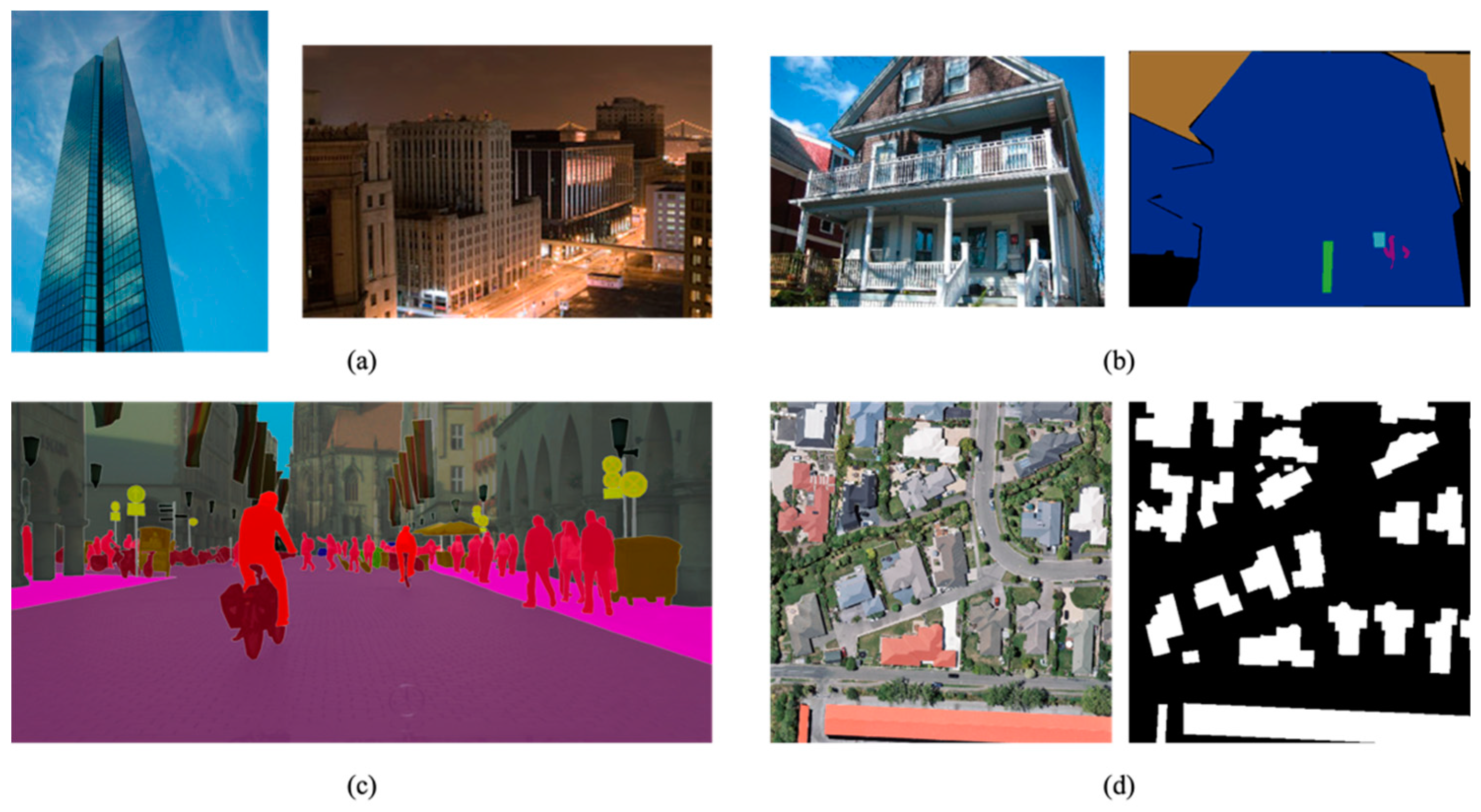
3.1. Experiment Data

The open-source building dataset WHU Building Dataset (WHU dataset) is used to compare DE-Net with other segmentation networks. The WHU dataset has 8189 tiles with 512 × 512 pixels and a spatial resolution of 0.3 m, and has been divided into three parts [43]: the training set, the validation set, and the testing set with 4736, 1036, and 2416 tiles, respectively. The whole dataset covers an area of 450 km² in New Zealand that contains more than 220,000 independent buildings with various appearance and usage. The rich data amount, appearance diversity, and label accuracy make it an ideal data source for model evaluation.

Considering that high-quality imagery and well-annotated training data such as the WHU dataset are expensive to obtain in real-world applications where the data source is often satellite imagery and the training samples are much less, we established a relatively small building dataset from GF-2 multispectral satellite imagery in Suzhou, China, covering an area of 8488 km², to evaluate the network performance in such a situation. GF-2 images have four bands—red, green, blue, and near-infrared—with a spatial resolution of 0.8 m. Thirty-two high-quality tiles of GF-2 images in 2017 were selected to remove the clouds and mosaicked together to construct the Suzhou satellite image, as shown in Figure 6. A total of 1184 images with 512 × 512 pixels were then cropped from the Suzhou satellite image and used to manually annotate the buildings in the images, comprising the Suzhou building dataset (Suzhou dataset). These images are randomly divided by 7:1:2 to constitute the training set, validation set, and testing set. The Suzhou dataset is much different from the WHU dataset in spatial resolution and imaging condition, as shown in Figure 7. The WHU dataset is better in sharpness, light, and color contrast. Images in the Suzhou dataset are less clear; the buildings are smaller, and many of them don’t have distinctly visible gaps in between.

3.2. Implementation Details

All the experiments are implemented by fastai v1 and PyTorch 1.0 with CUDA 10.0, ran by Nvidia GTX 1080Ti GPU. Random flipping and rotation are used for data augmentation. An adam optimizer [57] with a weight decay of 0.0000001 and one-cycle policy [58] are adopted in training. The learning rate is multiplied by 0.1 when the validation loss stops decreasing until it reaches 1 × 10⁻⁷. The initial learning rate is 0.01 for DE-Net and U-Net, since they are trained from scratch, and 0.0001 for SegNet, RefineNet, and DeepLab v3+, because they use pre-trained parameters. Note that on the Suzhou dataset, these three models are also trained from scratch, because GF-2 satellite images have four bands, while using a pre-trained model demands the input bands to be RGB.

3.3. Baseline Models

As mentioned in Section 3.2, the models that we re-implemented for evaluation are SegNet, U-Net, RefineNet, and DeepLab v3+. All these networks have an encoder–decoder structure and are fully convolutional. SegNet was originally proposed for a road scene and indoor scene segmentation. It uses the convolutional layers in VGG16 as its encoder, and the decoder is symmetrically constructed according to the encoder. SegNet also saves the max-pooling indices that are transmitted to the decoder to better recover the spatial information during upsampling. U-Net is designed to perform neuronal structure segmentation. The encoder block is simply double convolutional layers and a max-pooling layer. The decoder concatenates the feature maps in the corresponding encoder before convolution operation for precise localization. RefineNet is aimed to exploit the information along downsampling for high-resolution prediction. It employs short-range and long-range residual connections, multi-level fusion, and chained residual pooling for multi-path refinement. The specific version of RefineNet used in our experiments is RefineNet-Res101. DeepLab v3+ belongs to the DeepLab model family. The most innovative design in DeepLabs is the atrous convolution that expands the receptive fields without downsampling that loses spatial details. DeepLab v3+ adopts a new encoder–decoder structure that encodes multi-scale features by atrous convolution and better recovers fine detail in the decoder. RefineNet and DeepLab v3+ both achieved high performance in PASCAL VOC 2012 and Cityscapes datasets.

Besides the classic networks in computer vision, SRI-Net that is specifically designed for high-resolution building extraction has been evaluated on a WHU dataset in [47], and the result is referred to in our experiment for metric comparison. SRI-Net aggregates the multi-level outputs of the ResNet-101 encoder and then inputs the fused feature maps to the decoder enhanced by a spatial residual inception module.

3.4. Results on WHU Dataset

The WHU dataset covers a large variety of buildings, most of which are small residential blocks, and the rest are large buildings such as industrial factories and commercial buildings. Buildings have various shapes and textures, and an effective model must learn to recognize them from such complexity as good as possible. We trained SegNet, U-Net, RefineNet, DeepLab v3+, and DE-Net on the WHU dataset; the quantitative evaluation results are demonstrated in

Table 1. Quantitative evaluation results on the testing set of the WHU Building dataset (WHU dataset) by different models in terms of precision (%), recall (%), F1-Score (%), and intersection over union (IoU) (%) (best values are underlined).

Model	Precision	Recall	F1-Score	IoU
SegNet	$92.55\pm 0.23$	$93.06\pm 0.24$	$92.80\pm 0.24$	$86.58\pm 0.29$
U-Net	$93.83\pm 0.19$	$93.99\pm 0.21$	$93.91\pm 0.21$	$88.52\pm 0.26$
RefineNet	$94.24\pm 0.16$	$93.03\pm 0.21$	$93.63\pm 0.20$	$88.03\pm 0.25$
DeepLab v3+	$93.77\pm 0.17$	$93.46\pm 0.22$	$93.62\pm 0.21$	$88.00\pm 0.26$
SRI-Net (report) [47]	$95.21$	$93.28$	$94.24$	$89.09$
SRI-Net-UC (report) [47]	$\underset{-}{95.67}$	$93.69$	$94.51$	$89.23$
DE-Net	$95.00\pm 0.16$	$\underset{-}{94.60\pm 0.19}$	$\underset{-}{94.80\pm 0.18}$	$\underset{-}{90.12\pm 0.24}$

. Note that SRI-Net [47] is directly trained on the WHU dataset, and SRI-Net-UC is pre-trained on the University of California (UC) Merced Land Use Dataset and then trained on the WHU dataset. In [47], the standard error of each metric of SRI-Net on the WHU dataset is not provided, so that it is not presented in Table 1.

As shown in Table 1, SRI-Net-UC has the highest precision, and DE-Net achieves the highest and most stable recall, F1-Score, and IoU, which means that DE-Net is more balanced between precision and recall and achieves a better overall performance from the quantitative perspective. Interestingly, SegNet, RefineNet, and DeepLab v3+ that all have pre-trained parameters in their encoders are outperformed by models that trained from scratch, such as U-Net, SRI-Net, and DE-Net. Since the advantages of employing pre-trained parameters on ImageNet have been widely proved empirically in the field of semantic segmentation, it raises a question: Does this advantage still hold for high-resolution imagery building extraction tasks? Our thoughts are discussed in Section 4.1.

To visually demonstrate how these networks perform building extraction in different scenarios, some examples are shown in Figure 8. The first two rows are input images and ground truth images, and the following rows are building probability images predicted by SegNet, U-Net, RefineNet, DeepLab v3+, and DE-Net. Overall speaking, DE-Net produces the cleanest and most accurate results that don’t have much blurred content, which happens when the networks are not confident enough to discriminate buildings and give a moderate probability. It means that the structure of DE-Net is capable of learning the most representative features, although it doesn’t have a pre-trained powerful encoder, unlike SegNet, RefineNet, and DeepLab v3+. Column 1 shows that all five networks do well in small building recognition. However, as shown inside the red squares in column 2 to 5, DE-Net is the best for recovering the spatial detail and very robust for building roof color changing and tree covering. The results in the WHU dataset empirically indicate that the traditional downsampling procedure in VGGNet and ResNet and the upsampling methods in SegNet, U-Net, and DeepLab v3+ may not be the most appropriate settings for building extraction. With the existing large open-source datasets such as the WHU dataset, many new network structures can be invented and explored for better performance.

3.5. Results on Suzhou Building Dataset

Compared with Table 1, the performance of all networks drops drastically on the Suzhou dataset in

Table 2. Quantitative evaluation results on the testing set of the Suzhou building dataset (Suzhou dataset) by different models in terms of precision (%), recall (%), F1-Score (%), and IoU (%) (the best values are underlined).

Model	Precision	Recall	F1-Score	IoU
SegNet	$77.61\pm 2.09$	$72.75\pm 2.13$	$75.10\pm 2.10$	$60.13\pm 2.13$
U-Net	$82.19\pm 1.73$	$77.76\pm 1.77$	$79.92\pm 1.85$	$66.55\pm 1.92$
RefineNet	$76.77\pm 2.05$	$75.18\pm 1.96$	$75.97\pm 2.02$	$61.25\pm 2.06$
DeepLab v3+	$78.56\pm 1.77$	$75.21\pm 2.02$	$76.85\pm 1.93$	$62.40\pm 2.02$
DE-Net	$\underset{-}{85.11\pm 1.83}$	$\underset{-}{85.50\pm 1.69}$	$\underset{-}{85.31\pm 1.75}$	$\underset{-}{74.38\pm 1.85}$

. It is because the data quality of the Suzhou dataset is worse than that of the WHU dataset, and the buildings in the Suzhou dataset are more difficult to recognize. However, data with extremely high spatial resolution and clearness are hardly available in real-world applications. Nonetheless, there is still a relatively high DE-Net score in every metric, which leads other networks by a large margin. After we evaluate the network performance in the training set, it turns out that SegNet, U-Net, RefineNet, and DeepLab v3+ suffer from serious overfitting, in which every metric is at about 4% higher than the record on the testing set, as shown in

Table 3. Quantitative evaluation results on the training set of the Suzhou dataset by different models in terms of precision (%), recall (%), F1-Score (%), and IoU (%) (the best values are underlined).

Model	Precision	Recall	F1-Score	IoU
SegNet	$84.95\pm 0.47$	$77.62\pm 0.56$	$81.12\pm 0.51$	$68.23\pm 0.58$
U-Net	$\underset{-}{87.67\pm 0.40}$	$79.79\pm 0.46$	$83.55\pm 0.43$	$71.74\pm 0.52$
RefineNet	$82.00\pm 0.53$	$76.72\pm 0.57$	$79.27\pm 0.54$	$65.66\pm 0.60$
DeepLab v3+	$83.55\pm 0.48$	$76.15\pm 0.65$	$79.68\pm 0.59$	$66.22\pm 0.64$
DE-Net	$86.58\pm 0.42$	$\underset{-}{87.04\pm 0.42}$	$\underset{-}{86.81\pm 0.40}$	$\underset{-}{76.69\pm 0.49}$

, whereas DE-Net only increases by about 2%. The reason behind this is the inappropriate model complexity demonstrated in

Table 4. Complexity comparison of SegNet, U-Net, RefineNet, DeepLab v3+, and DE-Net (the lowest value is underlined).

Model	Parameters (m)	Training Time (Seconds/Epoch)
SegNet	$29.44$	$101$
U-Net	$13.38$	$72$
RefineNet	$113.88$	$160$
DeepLab v3+	$59.34$	$303$
DE-Net	$\underset{-}{9.63}$	$\underset{-}{81}$

. Models that are more complex have greater capacity, but they are also hard to train and prone to overfitting. VGG16 in SegNet and ResNet101 in DeepLab v3+ and RefineNet introduce a huge number of parameters, and such heavy structures hinder their performance when the pre-trained parameters are not provided. Their performance owes to the features learned from large-scale datasets such as ImageNet instead of the specific structures. The high scores of U-Net and DE-Net in Table 1, Table 2 and Table 3 prove that with enough training data, lighter networks that do not have pre-trained parameters possess the same power, or even better, for a specific task. It deserves great attention that building extraction is different from image classification, indoor scene segmentation, or road scene segmentation, and targeted network architecture innovation should be encouraged.

As in Section 3.3, some samples in the testing set are presented in Figure 9 for analysis. Figure 9 consists of images, ground truth images, and building probability images predicted by SegNet, U-Net, RefineNet, DeepLab v3+, and DE-Net from top to bottom, as in Figure 8. Some prediction images of SegNet, RefineNet, and DeepLab v3+ are blurred, because they are harder to converge given a small dataset and that the pre-trained parameters are deprived. On the contrary, the predictions of U-Net and DE-Net have a cleaner look. Column 1 is a residential neighborhood. In the corresponding ground truth, the thin gaps between each building in the same row are annotated, but all networks are unable to express such fine detail and separate these closely neighbored buildings. Even so, the roads between rows of buildings are well predicted by all networks. Column 2 depicts a similar case, and all networks can only recognize many small buildings as a whole object instead of many independent ones except for U-Net. U-Net separates some buildings but also loses certain parts, which is consistent with Table 2, that shows that U-Net achieves high precision and relatively low recall. Columns 3 and 4 are industrial buildings that are larger and distinctly separated. SegNet successfully detects large buildings, but misses many small buildings and makes a lot of wrong predictions. U-Net, RefineNet, and DeepLab v3+ show deficiency in recognizing large buildings. DE-Net delivers a satisfactory detection of buildings of various shapes and colors, which is also verified in column 5, showing that only DE-Net extracts the peculiar building completely. As the performance on unseen samples represents the generalization ability of a network, it can be concluded that DE-Net has the best generalization ability among all these networks in our experiments.

4. Discussion

4.1. How Necessary Is Fine-Tuning in Building Extraction?

Pre-trained parameters from image classification networks such as VGGNet and ResNet are commonly adopted as the segmentation network backbone in many segmentation researches and play an indispensable role in their high performance. To some extent, the success of such transfer learning relies on the similarity of data and problems. Indoor scenes and road scenes contain many objects that repeatedly appear in ImageNet, and they are all shot by cameras from a ground perspective, while remote sensing images are shot by aircraft from a top view, and only consist of certain objects such as buildings, roads, forests, water areas, and ground. As a result, the pre-trained parameters may not well represent the target objects in remote sensing imagery. In addition, some sensors produce multiple bands rather than RGB bands. To take advantage of the pre-trained parameters in such conditions, only the RGB bands can be utilized, and the valuable information in the rest of the bands has to be discarded.

In our experiments on the WHU dataset and Suzhou dataset, it suggests that such a trade-off is not necessary for better performance. DE-Net was constructed and trained from scratch and outperforms SegNet, RefineNet, and DeepLab v3+ on both datasets, as illustrated in Section 3. Besides, with the contribution of pre-trained parameters, their performance was still slightly worse than U-Net on the WHU dataset. When it comes to the Suzhou dataset, in which all the networks were trained from scratch, these three networks performed way worse than U-Net and DE-Net, indicating that their structures are internally unsuitable for building extraction on these two datasets. Unfortunately, training a deep network model needs lots of data. When the available data are insufficient, fine-tuning a pre-trained network could help, and parameters that pre-trained on a related large-scale dataset are preferred to those trained on an irrelevant dataset. For instance, tasks related to building extraction can design a new network and pre-train it on the WHU dataset, instead of the CityScape dataset or PASCAL VOC, and then fine-tune it. Future works on building extraction could explore more possibilities of network architecture.

4.2. Self-Comparison Study on DE-Net

The design of DE-Net is motivated by the insights of many current deep convolutional neural networks. We’ve tried plenty of options before the final structure. To demonstrate the influence of each component in DE-Net, we present the quantitative evaluation results of some representative variation of DE-Net in

Table 5. DE-Net self-comparison study results on the testing set of the WHU dataset in terms of F1-Score (%) (the different component from the baseline model are underlined).

Depth of Encoding Module	Upsampling Method	Channel Dimension	Activation Functions	Loss Function	F1-Score
6	DUC 1	128, 256, 512	ReLU + SELU 2	Dice + BCE 3	$94.80$
4	DUC	128, 256, 512	ReLU + SELU	Dice + BCE	$93.99$
5	DUC	128, 256, 512	ReLU + SELU	Dice + BCE	$94.45$
7	DUC	128, 256, 512	ReLU + SELU	Dice + BCE	$93.74$
6	U-Net Schema	128, 256, 512	ReLU + SELU	Dice + BCE	$93.80$
6	DUC	64, 128, 256	ReLU + SELU	Dice + BCE	$94.10$
6	DUC	256, 512, 1024	ReLU + SELU	Dice + BCE	$93.54$
6	DUC	128, 256, 512	ReLU4	Dice + BCE	$93.75$
6	DUC	128, 256, 512	PReLU4	Dice + BCE	$94.00$
6	DUC	128, 256, 512	ELU4	Dice + BCE	$93.59$
6	DUC	128, 256, 512	SELU4	Dice + BCE	$94.05$
6	DUC	128, 256, 512	ReLU + PReLU5	Dice + BCE	$94.38$
6	DUC	128, 256, 512	ReLU + SELU	BCE	$93.95$

¹ Densely upsampling convolution. ² ReLU in downsampling and compressing modules and SELU in encoding modules. ³ Dice and binary cross-entropy loss. ⁴ The same activation function used throughout the whole network. ⁵ ReLU in downsampling and compressing modules and PReLU in encoding modules.

. The first row is the baseline DE-Net that appears in prior sections. Each of the following rows has only one component different from the first row. The depth of an encoding module is the number of linear residual blocks used in the encoding module, as explained in Section 2.3. The upsampling method is used to recover the spatial information. The channel dimension is how the channel of feature maps expands. The expansion operations are carried out in downsampling modules, and between each expansion is an encoding module. The performance of all models is illustrated with an F1-Score. The difference in the first four models is the depth of encoding modules. It shows that the depths shallower or deeper than six all worsen the performance. Although network depth contributes a lot to network capacity, it has an optimal value for a specific network architecture, not to mention the additional memory consumption caused by increasing network depth. The next model upsamples feature maps such as U-Net that concatenate feature maps in the encoder and use the deconvolutional layer to recover spatial resolution, resulting in a 1% drop in F1-Score. The feature channel is explored in the next two models. A thinner model may be deficient in representation capacity, and a wider model may be harder to converge; thus, the performance is restricted. As discussed in Section 2.2, activation functions play an important role in information propagation inside a network. According to the next five models, the optimal setting of activation function in DE-Net is to use ReLU in downsampling modules and SELU in encoding modules. The last model shows that combining dice and binary cross-entropy loss increases the F1-Score by about 0.9%.

5. Conclusions

In this paper, we propose a fully convolutional network DE-Net for building extraction from high-resolution remote sensing imagery. DE-Net is designed for information preservation through network computation, especially in downsampling, encoding, and upsampling procedures. Its main innovations are as follows: (1) The downsampling operation combines striding convolution and max pooling. (2) In its encoding modules, the SELU activation function is used instead of a commonly used ReLU. (3) DE-Net doesn’t upsample feature maps by bilinear interpolation or deconvolution; it uses the densely upsampling convolution module that enables DE-Net to encode complete spatial information in feature maps for pixel-wise prediction. Besides, DE-Net is trained by dice and cross-entropy loss to address the class imbalance problem.

We compare DE-Net with other image segmentation networks on a public dataset WHU dataset consisting of aerial images and a self-built dataset Suzhou dataset consisting of GF-2 satellite images. Although these two datasets have different data attributes and building appearances, DE-Net achieves the best results without any pre-trained parameters on both datasets, proving its internal effectiveness on building extraction on two commonly used remote sensing image data sources. As the visual prediction examples demonstrate, DE-Net outputs the most accurate spatial detail, and is less affected by noises such as a building roof color changing or tree covering. Besides, on the Suzhou dataset that has lower imagery quality and training samples, DE-Net still succeeds in predicting most of the buildings varying in sizes and shapes.

The outstanding performance of DE-Net leads to doubt on the necessity of fine-tuning a network pre-trained on datasets irrelevant to building extraction. According to our experimental results, we conclude that large-scale datasets such as the WHU dataset are preferable pre-training data sources. For multispectral data that lack corresponding large-scale datasets, designing a new network based on the particular task may deliver better results compared with using an existing network that performs well on an unrelated problem. We also inspected the most influential factors and hopefully help some future research concerning network architecture innovation.

To further improve the performance of DE-Net, many lately emerging techniques can be integrated, such as group normalization and generative adversarial training. Given that building extraction is a subproblem of image segmentation, future research may explore how DE-Net performs on classifying other land-cover types such as water area, forest, roads, etc. Moreover, since DE-Net has no restriction on the input band number, therefore, it is very easy to apply it to other kinds of data sources, e.g., multispectral data and synthetic aperture radar data, and it also remains the potential in data fusion.

References

1. Bettencourt, L.; West, G. A unified theory of urban living. Nature. 2010, 467, 912–913. [Google Scholar] [CrossRef] [PubMed]
2. Yang, H.L.; Yuan, J.; Lunga, D.; Laverdiere, M.; Rose, A.; Bhaduri, B. Building extraction at scale using convolutional neural network: Mapping of the united states. IEEE J. Sel. Top. Appl. Earth Obs. Remote Sens. 2018, 11, 2600–2614. [Google Scholar] [CrossRef]
3. Huang, B.; Zhao, B.; Song, Y. Urban land-use mapping using a deep convolutional neural network with high spatial resolution multispectral remote sensing imagery. Remote Sens. Environ. 2018, 214, 73–86. [Google Scholar] [CrossRef]
4. Amado, M.; Poggi, F.; Amado, A.R. Energy efficient city: A model for urban planning. Sustain. Cities Soc. 2016, 26, 476–485. [Google Scholar] [CrossRef]
5. Xiao, P.; Yuan, M.; Zhang, X.; Feng, X.; Guo, Y. Cosegmentation for object-based building change detection from high-resolution remotely sensed images. IEEE Trans. Geosci. Remote Sens. 2017, 55, 1587–1603. [Google Scholar] [CrossRef]
6. Xie, Y.; Weng, A.; Weng, Q. Population estimation of urban residential communities using remotely sensed morphologic data. IEEE Geosci. Remote Sens. Lett. 2015, 12, 1111–1115. [Google Scholar]
7. Sirmacek, B.; Unsalan, C. Building detection from aerial images using invariant color features and shadow information. In Proceedings of the 23rd International Symposium on Computer and Information Sciences, Istanbul, Turkey, 27–29 October 2008; pp. 1–5. [Google Scholar] [CrossRef]
8. Zhang, Y. Optimisation of building detection in satellite images by combining multispectral classification and texture filtering. ISPRS J. Photogramm. Remote Sens. 1999, 54, 50–60. [Google Scholar] [CrossRef]
9. Dunaeva, A.V.e.; Kornilov, F.A. Specific shape building detection from aerial imagery in infrared range. Vestnik Yuzhno-Ural’skogo Gosudarstvennogo Universiteta. Seriya “Vychislitelnaya Matematika i Informatika” 2017, 6, 84–100. [Google Scholar]
10. Li, Y.; Wu, H. Adaptive building edge detection by combining LiDAR data and aerial images. Int. Arch. Photogramm. Remote Sens. Spat. Inf. Sci. 2008, 37, 197–202. [Google Scholar]
11. Ok, A.O.; Senaras, C.; Yuksel, B. Automated detection of arbitrarily shaped buildings in complex environments from monocular VHR optical satellite imagery. IEEE Trans. Geosci. Remote Sens. 2012, 51, 1701–1717. [Google Scholar] [CrossRef]
12. Huang, X.; Zhang, L.; Zhu, T. Building change detection from multitemporal high-resolution remotely sensed images based on a morphological building index. IEEE J. Sel. Top. Appl. Earth Obs. Remote Sens. 2013, 7, 105–115. [Google Scholar] [CrossRef]
13. Lecun, Y.; Boser, B.; Denker, J.; Henderson, D.; Howard, R.E.; Hubbard, W.; Jackel, L. Backpropagation Applied to Handwritten Zip Code Recognition. Neural Comput. 1989, 1, 541–551. [Google Scholar] [CrossRef]
14. LeCun, Y.; Bottou, L.; Bengio, Y.; Haffner, P. Gradient-based learning applied to document recognition. Proc. IEEE 1998, 86, 2278–2324. [Google Scholar] [CrossRef] [Green Version]
15. Deng, J.; Dong, W.; Socher, R.; Li, L.-J.; Li, K.; Fei-Fei, L. Imagenet: A large-scale hierarchical image database. In Proceedings of the 2009 IEEE Conference on Computer Vision and Pattern Recognition, Miami, FL, USA, 20–25 June 2009; pp. 248–255. [Google Scholar]
16. Everingham, M.; Van Gool, L.; Williams, C.K.; Winn, J.; Zisserman, A. The pascal visual object classes (voc) challenge. Int. J. Comput. Vis. 2010, 88, 303–338. [Google Scholar] [CrossRef]
17. Zhou, B.; Zhao, H.; Puig, X.; Xiao, T.; Fidler, S.; Barriuso, A.; Torralba, A. Semantic understanding of scenes through the ade20k dataset. Int. J. Comput. Vis. 2019, 127, 302–321. [Google Scholar] [CrossRef]
18. Cordts, M.; Omran, M.; Ramos, S.; Rehfeld, T.; Enzweiler, M.; Benenson, R.; Franke, U.; Roth, S.; Schiele, B. The cityscapes dataset for semantic urban scene understanding. In Proceedings of the IEEE conference on Computer Vision and Pattern Recognition, Las Vegas, NV, USA, 27–30 June 2016; pp. 3213–3223. [Google Scholar]
19. Krizhevsky, A.; Sutskever, I.; Hinton, G.E. Imagenet classification with deep convolutional neural networks. In Proceedings of the Advances in Neural Information Processing Systems, Lake Tahoe, Nevada, 3–6 December 2012; pp. 1097–1105. [Google Scholar]
20. Szegedy, C.; Liu, W.; Jia, Y.; Sermanet, P.; Reed, S.; Anguelov, D.; Erhan, D.; Vanhoucke, V.; Rabinovich, A. Going deeper with convolutions. In Proceedings of the IEEE Conference on Computer Vision and Pattern Recognition (CVPR), Boston, MA, USA, 7–12 June 2015; pp. 1–9. [Google Scholar] [CrossRef]
21. Simonyan, K.; Zisserman, A. Very deep convolutional networks for large-scale image recognition. arXiv 2014, arXiv:1409.1556. [Google Scholar]
22. He, K.; Zhang, X.; Ren, S.; Sun, J. Deep Residual Learning for Image Recognition. In Proceedings of the IEEE Conference on Computer Vision and Pattern Recognition (CVPR), Las Vegas, NV, USA, 27–30 June 2016; pp. 770–778. [Google Scholar] [CrossRef]
23. Long, J.; Shelhamer, E.; Darrell, T. Fully convolutional networks for semantic segmentation. In Proceedings of the IEEE Conference on Computer Vision and Pattern Recognition, Boston, MA, USA, 7–12 June 2015; pp. 3431–3440. [Google Scholar]
24. Ronneberger, O.; Fischer, P.; Brox, T. U-net: Convolutional networks for biomedical image segmentation. In Proceedings of the International Conference on Medical Image Computing and Computer-Assisted Intervention, Granada, Spain, 16–20 September 2018; pp. 234–241. [Google Scholar]
25. Badrinarayanan, V.; Kendall, A.; Cipolla, R. SegNet: A Deep Convolutional Encoder-Decoder Architecture for Image Segmentation. IEEE Trans. Pattern Anal. Mach. Intell. 2017, 39, 2481–2495. [Google Scholar] [CrossRef]
26. Chen, L.-C.; Papandreou, G.; Kokkinos, I.; Murphy, K.; Yuille, A.L. DeepLab: Semantic Image Segmentation with Deep Convolutional Nets, Atrous Convolution, and Fully Connected CRFs. IEEE Trans. Pattern Anal. Mach. Intell. 2017, 40, 834–848. [Google Scholar] [CrossRef]
27. Zhao, H.; Shi, J.; Qi, X.; Wang, X.; Jia, J. Pyramid Scene Parsing Network. In Proceedings of the IEEE Conference on Computer Vision and Pattern Recognition (CVPR), Honolulu, HI, USA, 21–26 July 2017; pp. 6230–6239. [Google Scholar] [CrossRef]
28. Girshick, R.; Donahue, J.; Darrell, T.; Malik, J. Rich feature hierarchies for accurate object detection and semantic segmentation. In Proceedings of the 2014 IEEE Conference on Computer Vision and Pattern Recognition, Columbus, OH, USA, 23–28 June 2014. [Google Scholar]
29. Yoo, D.; Park, S.; Lee, J.-Y.; Paek, A.S.; So Kweon, I. Attentionnet: Aggregating weak directions for accurate object detection. In Proceedings of the IEEE International Conference on Computer Vision, Santiago, Chile, 7–13 December 2015; pp. 2659–2667. [Google Scholar]
30. Ren, S.; He, K.; Girshick, R.; Sun, J. Faster r-cnn: Towards real-time object detection with region proposal networks. In Proceedings of the Advances in neural information processing systems, Vancouver, BC, Canada, 3–6 December 2007; pp. 91–99. [Google Scholar]
31. Redmon, J.; Divvala, S.; Girshick, R.; Farhadi, A. You Only Look Once: Unified, Real-Time Object Detection. In Proceedings of the 2016 IEEE Conference on Computer Vision and Pattern Recognition (CVPR), Las Vegas, NV, USA, 27–30 June 2016; pp. 779–788. [Google Scholar] [CrossRef]
32. He, K.; Gkioxari, G.; Dollar, P.; Girshick, R. Mask R-CNN. In Proceedings of the 2017 IEEE International Conference on Computer Vision (ICCV), Venice, Italy, 22–29 October 2017; pp. 2980–2988. [Google Scholar]
33. Zeiler, M.D.; Fergus, R. Visualizing and Understanding Convolutional Networks; Springer: Cham, Switzerland, 2014; Volume 8689, pp. 818–833. [Google Scholar]
34. LeCun, Y.; Bengio, Y.; Hinton, G. Deep learning. Nature 2015, 521, 436. [Google Scholar] [CrossRef]
35. Huh, M.; Agrawal, P.; Efros, A.A. What makes ImageNet good for transfer learning? arXiv 2016, arXiv:1608.08614. [Google Scholar]
36. Shrestha, S.; Vanneschi, L. Improved fully convolutional network with conditional random fields for building extraction. Remote Sens. 2018, 10, 1135. [Google Scholar] [CrossRef]
37. Lu, T.; Ming, D.; Lin, X.; Hong, Z.; Bai, X.; Fang, J. Detecting building edges from high spatial resolution remote sensing imagery using richer convolution features network. Remote Sens. 2018, 10, 1496. [Google Scholar] [CrossRef]
38. Wu, G.; Guo, Z.; Shi, X.; Chen, Q.; Xu, Y.; Shibasaki, R.; Shao, X. A boundary regulated network for accurate roof segmentation and outline extraction. Remote Sens. 2018, 10, 1195. [Google Scholar] [CrossRef]
39. Zhang, Z.; Wang, Y. JointNet: A Common Neural Network for Road and Building Extraction. Remote Sens. 2019, 11, 696. [Google Scholar] [CrossRef]
40. Mnih, V. Machine Learning for Aerial Image Labeling; University of Toronto (Canada): Toronto, ON, Canada, 2013. [Google Scholar]
41. Rottensteiner, F.; Sohn, G.; Jung, J.; Gerke, M.; Baillard, C.; Benitez, S.; Breitkopf, U. The ISPRS benchmark on urban object classification and 3D building reconstruction. ISPRS Ann. Photogramm. Remote Sens. Spat. Inf. Sci. 2012, 1, 293–298. [Google Scholar] [CrossRef]
42. Maggiori, E.; Tarabalka, Y.; Charpiat, G.; Alliez, P. Can semantic labeling methods generalize to any city? the inria aerial image labeling benchmark. In Proceedings of the 2017 IEEE International Geoscience and Remote Sensing Symposium (IGARSS), Fort Worth, TX, USA, 23–28 July 2017; pp. 3226–3229. [Google Scholar]
43. Ji, S.; Wei, S.; Lu, M. Fully convolutional networks for multisource building extraction from an open aerial and satellite imagery data set. IEEE Trans. Geosci. Remote Sens. 2018, 57, 574–586. [Google Scholar] [CrossRef]
44. Saito, S.; Yamashita, T.; Aoki, Y. Multiple object extraction from aerial imagery with convolutional neural networks. Electron. Imaging 2016, 2016, 1–9. [Google Scholar] [CrossRef]
45. Alshehhi, R.; Marpu, P.R.; Woon, W.L.; Dalla Mura, M. Simultaneous extraction of roads and buildings in remote sensing imagery with convolutional neural networks. ISPRS J. Photogramm. Remote Sens. 2017, 130, 139–149. [Google Scholar] [CrossRef]
46. Maggiori, E.; Tarabalka, Y.; Charpiat, G.; Alliez, P. Convolutional neural networks for large-scale remote-sensing image classification. IEEE Trans. Geosci. Remote Sens. 2016, 55, 645–657. [Google Scholar] [CrossRef]
47. Liu, P.; Liu, X.; Liu, M.; Shi, Q.; Yang, J.; Xu, X.; Zhang, Y. Building Footprint Extraction from High-Resolution Images via Spatial Residual Inception Convolutional Neural Network. Remote Sens. 2019, 11, 830. [Google Scholar] [CrossRef]
48. Marmanis, D.; Schindler, K.; Wegner, J.D.; Galliani, S.; Datcu, M.; Stilla, U. Classification with an edge: Improving semantic image segmentation with boundary detection. ISPRS J. Photogramm. Remote Sens. 2018, 135, 158–172. [Google Scholar] [CrossRef] [Green Version]
49. Lin, G.; Milan, A.; Shen, C.; Reid, I. Refinenet: Multi-path refinement networks for high-resolution semantic segmentation. In Proceedings of the IEEE conference on Computer Vision and Pattern Recognition, Honolulu, HI, USA, 21–26 July 2017; pp. 1925–1934. [Google Scholar]
50. Chen, L.-C.; Zhu, Y.; Papandreou, G.; Schroff, F.; Adam, H. Encoder-decoder with atrous separable convolution for semantic image segmentation. In Proceedings of the European Conference on Computer Vision (ECCV), Munich, Germany, 8–14 September 2018; pp. 801–818. [Google Scholar]
51. Klambauer, G.; Unterthiner, T.; Mayr, A.; Hochreiter, S. Self-normalizing neural networks. In Proceedings of the Advances in Neural Information Processing Systems, Long Beach, CA, USA, 4–9 December 2017; pp. 971–980. [Google Scholar]
52. Nair, V.; Hinton, G.E. Rectified linear units improve restricted boltzmann machines. In Proceedings of the 27th international Conference on Machine Learning (ICML-10), Haifa, Israel, 21–24 June 2010; pp. 807–814. [Google Scholar]
53. He, K.; Zhang, X.; Ren, S.; Sun, J. Delving deep into rectifiers: Surpassing human-level performance on imagenet classification. In Proceedings of the IEEE International Conference on Computer Vision, Santiago, Chile, 7–13 December 2015; pp. 1026–1034. [Google Scholar]
54. Clevert, D.-A.; Unterthiner, T.; Hochreiter, S. Fast and accurate deep network learning by exponential linear units (elus). arXiv 2015, arXiv:1511.07289. [Google Scholar]
55. Sandler, M.; Howard, A.; Zhu, M.; Zhmoginov, A.; Chen, L.-C. MobileNetV2: Inverted Residuals and Linear Bottlenecks. In Proceedings of the 2018 IEEE/CVF Conference on Computer Vision and Pattern Recognition, Salt Lake City, UT, USA, 18–23 June 2018; pp. 4510–4520. [Google Scholar] [CrossRef]
56. Wang, P.; Chen, P.; Yuan, Y.; Liu, D.; Huang, Z.; Hou, X.; Cottrell, G. Understanding Convolution for Semantic Segmentation. In Proceedings of the 2018 IEEE Winter Conference on Applications of Computer Vision, Lake Tahoe, NV, USA, 12–15 March 2018; pp. 1451–1460. [Google Scholar] [CrossRef]
57. Kingma, D.P.; Ba, J. Adam: A method for stochastic optimization. arXiv 2014, arXiv:1412.6980. [Google Scholar]
58. Smith, L.N. Cyclical learning rates for training neural networks. In Proceedings of the 2017 IEEE Winter Conference on Applications of Computer Vision (WACV), Santa Rosa, CA, USA, 24–31 March 2017; pp. 464–472. [Google Scholar]
Figure 1. Different building-related datasets. (a) ImageNet dataset, training VGGNet and ResNet. (b) ADE20K dataset, training PSPNet. (c) Cityscapes, training SegNet and DeepLab. (d) WHU Building Dataset.
Remotesensing 11 02380 g001
Figure 2. Overview of the Deep Encoding Network (DE-Net).
Remotesensing 11 02380 g002
Figure 3. Functions including exponential linear unit (ELU), parametric rectified linear unit (PReLU), rectified linear unit (ReLU), and scaled exponential linear unit (SELU).
Remotesensing 11 02380 g003
Figure 4. Modules of DE-Net. (a) Linear residual block activated by SELU, basic blocks of the encoding module. (b) Downsampling module. (c) Compressing module.
Remotesensing 11 02380 g004
Figure 5. Densly upsampling convolution (DUC).
Remotesensing 11 02380 g005
Figure 6. GF-2 multispectral satellite imagery in Suzhou.
Remotesensing 11 02380 g006
Figure 7. Examples of (a) WHU Building Dataset (WHU dataset) and (b) Suzhou building dataset (Suzhou dataset), divided by column.
Remotesensing 11 02380 g007
Figure 8. Building extraction results on the WHU dataset. The first two rows are images and corresponding ground truth. The rest five rows are produced by SegNet, U-Net, RefineNet, DeepLab v3+, and DE-Net.
Remotesensing 11 02380 g008
Figure 9. Building extraction results on the Suzhou dataset. The first two rows are images and corresponding ground truth. The rest five rows are produced by SegNet, U-Net, RefineNet, DeepLab v3+, and DE-Net.
Remotesensing 11 02380 g009