Article

A Bidirectional Analysis Method for Extracting Glacier Crevasses from Airborne LiDAR Point Clouds

1
State Key Laboratory of Geodesy and Earth’s Dynamics, Institute of Geodesy and Geophysics, Chinese Academy of Sciences, Wuhan 430077, China
2
College of Earth and Planetary Sciences, University of Chinese Academy of Sciences, Beijing 100049, China
3
State Key Laboratory of Information Engineering in Surveying, Mapping and Remote Sensing, Wuhan University, Wuhan 430077, China
*
Author to whom correspondence should be addressed.
Remote Sens. 2019, 11(20), 2373; https://doi.org/10.3390/rs11202373
Submission received: 15 August 2019 / Revised: 7 October 2019 / Accepted: 9 October 2019 / Published: 13 October 2019
(This article belongs to the Special Issue Applications of Remote Sensing in Glaciology)

Abstract

:
A crevasse is an important surface feature of a glacier. This study aims to detect crevasses from high-density airborne LiDAR point clouds. However, existing methods continue to suffer from the data holes within the crevasse region and the influence of the undulating non-crevasse glacier surfaces. Therefore, a bidirectional analysis method is proposed to robustly extract the crevasses from the point clouds, which utilizes their vertical and horizontal characteristics. First, crevasse points are separated from non-crevasse points using a hybrid-entity method, where the height difference and the nearly vertical characteristic of a crevasse sidewall are considered, to better distinguish the crevasses from the undulating non-crevasse glacier surfaces. Second, the crevasse regions/edges are adaptively delineated by a local statistical analysis method that is based on a novel feature of the Delaunay triangulation mesh of non-crevasse points in the horizontal plane. Last, the pseudo-crevasse points and regions are removed by a cross-analysis method. To test the performance of the proposed method, this study selected airborne LiDAR point clouds from two sites of Alaskan glaciers (i.e., Tyndall Glacier and Seward Glacier) as the experimental datasets. The results were verified by a comparison with the ground truth that was manually delineated. The proposed method achieved acceptable results: the recall, precision, and F 1 scores of both sites exceeded 94.00%. Moreover, a comparative experiment was carried out and the results confirmed that the proposed method achieved superior performance.

1. Introduction

As a visible surface feature of glacier ice, crevasses form when a yield tensile stress or critical strain rate is reached, and they are frequently distributed on glaciers, ice sheets and ice shelves [1,2]. These crevasses can be taken as markers in the feature tracking methods to measure the ice velocity. Crevasses are also important pathways for transmitting glacier surface water to an englacial hydrological network and bedrocks [3,4,5,6], which consequently have a significant influence on ice dynamics due to an increase in basal lubrication [7]. Moreover, the propagation of crevasses has a key role in the calving of the vicinity of the ice front [8]. Therefore, the detection of surface crevasses is critical for these further applications of crevasses to understand both the ice dynamic and the mass balance on glaciers and ice sheets.
In past decades, two different means (i.e., field studies and remote sensing studies) have been employed to observe crevasses. Comparatively speaking, remote sensing techniques have become more important tools, while field studies are severely limited because crevasses pose a serious safety hazard [7,9]. In the last two decades, multi-source remote sensing data (e.g., optical images, synthetic aperture radar (SAR), and LiDAR) obtained by aircraft and satellites have been applied to detect crevasses [9,10,11,12,13]. For most of these methods, only two-dimensional crevasses are obtained. However, three-dimensional crevasses are necessary for some glacier studies (e.g., the hydrological process and calving). For example, third-dimensional information (i.e., depth) of a crevasse is a key parameter in some physically-based calving models [8]. To obtain three-dimensional crevasses, researchers have attempted to employ new techniques and sensors, such as satellite altimeters, stereophotogrammetry, and laser scanning. Liu et al. [12] detected sparse crevasse points from three-dimensional ICESat-1/GLAS footprints for large-size crevasses. Other researchers reconstructed three-dimensional information of glacier surfaces using stereophotogrammetry [14,15,16,17], and three-dimensional crevasses can also be captured [18,19]. Although these stereophotogrammetry methods are efficient for the three-dimensional mapping of crevasses, they are still limited by three factors: (1) The difficulty of surveying evenly distributed ground control points; (2) the low contrast of the texture over a glacier surface; and (3) the lack of light at the bottom and sidewalls of a crevasse. To overcome these issues, some researchers have attempted to map crevasses using laser scanning systems [20,21,22], regardless of the low contrast of the glacier surface texture and the shadow within the region of a crevasse.
Laser scanning systems, including terrestrial laser scanning (TLS) and the Airborne LiDAR System (ALS), can directly acquire high-precision and high-density three-dimensional point clouds of a glacier surface [23] and they have been applied in the observation of glacier geomorphology, ice flow, mass balance and calving [24,25,26]. However, ALS can be better than TLS in the observation of crevasses due to its scanning position and angle and has a greater opportunity to acquire more data of crevasse sidewalls and bottoms. With the development of a low-cost unmanned aerial vehicle (UAV) ALS system, ALS will receive an increasing amount of attention in the cryosphere [10,27], especially for the high spatio-temporal resolution observations of the alpine small glacier and the front of a calving glacier. To automatically detect crevasses from LiDAR data, researchers have proposed the point-based methods and the digital elevation model (DEM)-based methods [20,21,22,24,28], which are primarily based on height-related features. Generally, these methods can obtain suitable results when a non-crevasse glacier surface is smooth and a crevasse is perfectly measured. However, these methods suffer from the influences of undulating non-crevasse surfaces and data holes within the crevasse regions. Distinguishing undulating non-crevasse surfaces from the crevasses only based on the height-related features in these methods is difficult. The data holes can also affect the extraction of crevasses. More specially, the interpolation of the data hole causes the omission of crevasse detection and the location errors of the crevasse boundaries in DEM-based methods, and the detected crevasse is not complete by the existing point-based methods due to the data holes within the crevasse regions. Fortunately, the crevasse has other special characteristics, with the exception of the depth, including the nearly vertical sidewalls and the opening width, which is helpful for improving the quality of crevasses detection.
Therefore, this study proposes a bidirectional analysis method for detecting crevasses from airborne LiDAR point clouds. First, crevasse points are separated from non-crevasse points by a hybrid-entity method, which utilizes the height difference between the crevasse point and its neighboring non-crevasse points and the nearly vertical crevasse sidewalls. Second, the crevasse edges/regions are extracted from the non-crevasse points using a local statistical analysis method, according to the assumption that the crevasse width is larger than the average point spacing in this study. Last, a cross-analysis method is carried out to remove the pseudo-crevasse points and regions.
The rest of this paper is organized as follows. The study area and datasets are presented in Section 2. Section 3 describes the proposed methodology. In Section 4, the results are presented. A discussion and our conclusions are presented in Section 5 and Section 6, respectively.

2. Study Area and Datasets

2.1. Study Area

The study area includes two sites which are located in two Alaskan glaciers, as shown in Figure 1. The first site is located on Malaspina Glacier in southeastern Alaska. Malaspina Glacier is a compound glacier that consists of several valley glaciers, including Agassiz Glacier and Seward Glacier. At this site, the local terrain is smooth, and the distribution of the directions of the crevasses is relatively unified. The second site is located on Tyndall Glacier, which is an intersection point between two valley glaciers, where the slope is steep. The glacier surface is heavily crevassed at this site, and the directions of the crevasses are various. Moreover, the phenomenon that the widths of the crevasses are largely different exists in both sites. The maximum width can be dozens of meters, while some small crevasses are very narrow.

2.2. Experimental Datasets

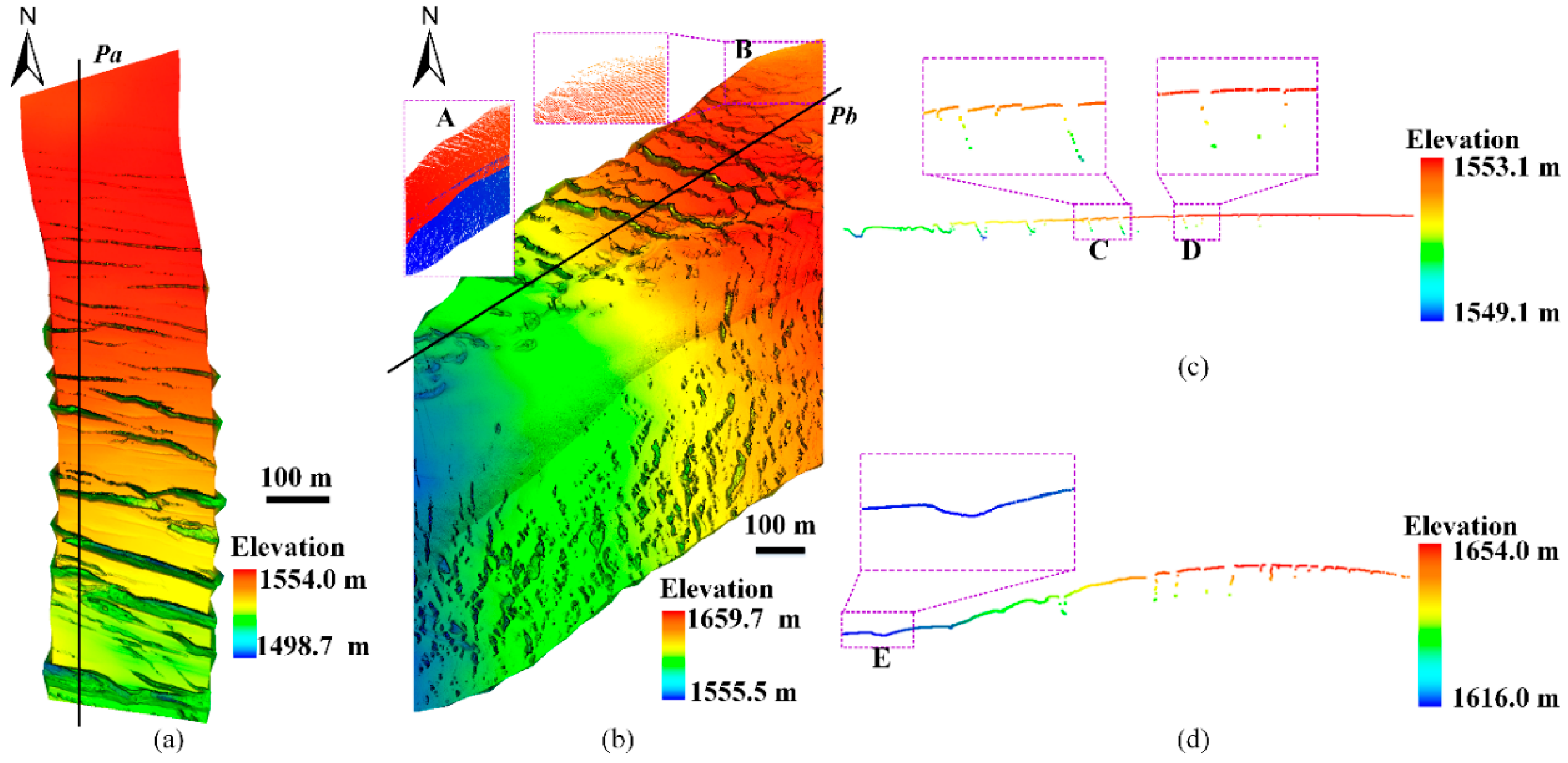
In this study, the University of Alaska Fairbanks (UAF) LiDAR Scanner L1B (ILAKS1B) Geolocated Surface Elevation Triplets dataset [29], which was acquired by the UAF airborne LiDAR system, was employed. The general configuration of the UAF flight campaigns is listed in Table 1. The point clouds of the two sites are displayed in Figure 2. The details are listed as following: (Ⅰ) The first site (Site 1) has an area of 1.09 × 0.25 km2. It is a part of a single strip acquired on 22 August 2009, and the point density is relatively uniform. However, the crevasse detection method faces two challenges at this site: The crevasse sidewall points are only found on one sidewall for most of the crevasses, as shown in local view C of Figure 2. When the width of a crevasse is too small, the points of the crevasse sidewalls and bottom are very few and sparse, as shown in local view D of Figure 2. (Ⅱ) The second site (Site 2) covers 0.65 × 0.82 km2 and consists of two strips acquired on 22 August 2009. The point clouds of the two strips are marked in different colors as shown in rectangle A of Figure 2. In addition to the challenges posed by the first site, the proposed method faces three additional challenges: the uneven point density, the undulating non-crevasse glacier surface and the data holes on non-crevasse glacier surfaces, as shown in rectangles A, E, and B in Figure 2. In summary, many challenges exist for automatically extracting crevasses on these two sites, and these two sites are suitable to test the performance of the proposed method.

3. Methodology

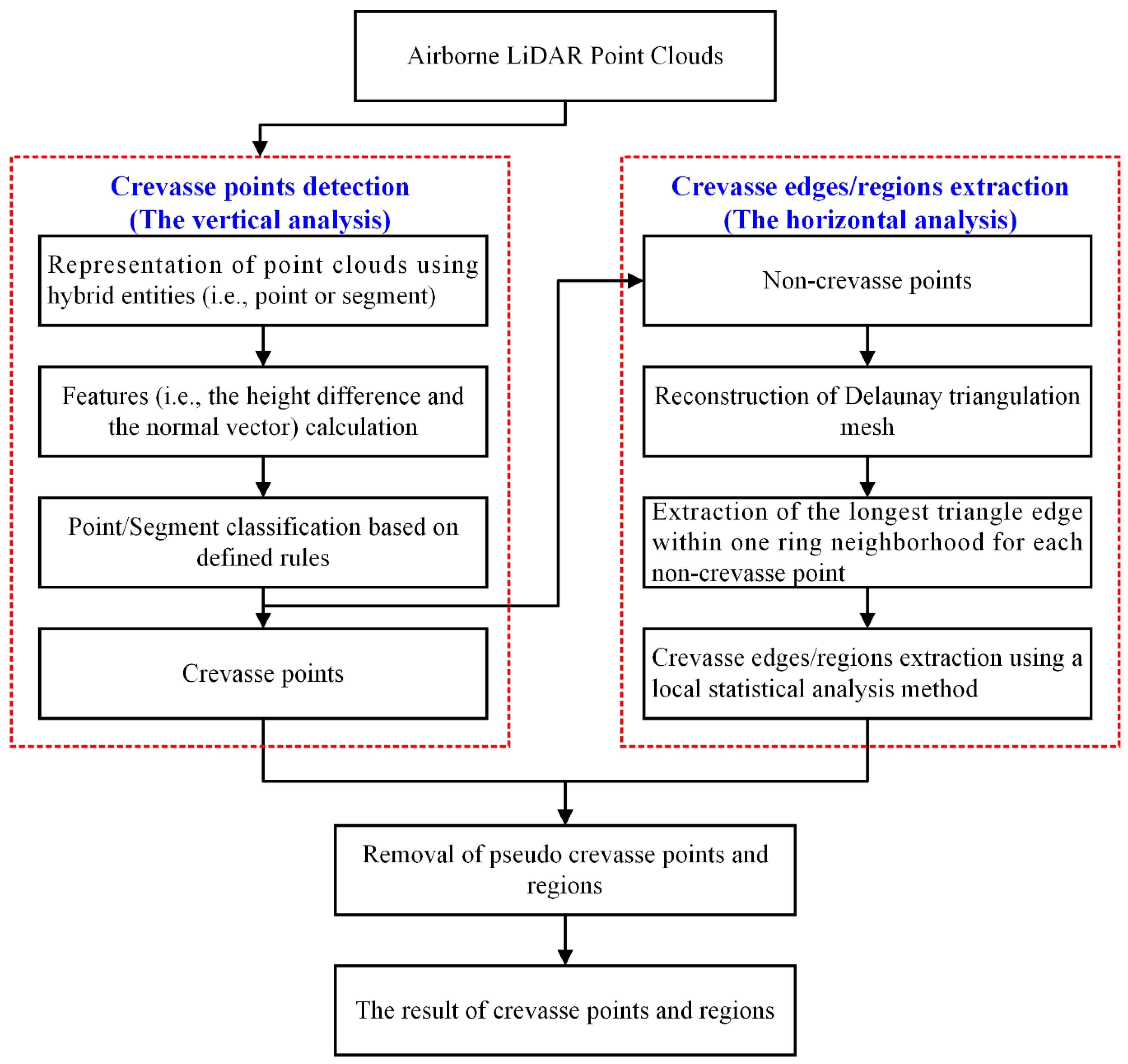
Figure 3 illustrates the workflow of the bidirectional analysis method. The proposed method is composed of three key steps: crevasse points detection, crevasse edges/regions extraction, and the removal of the pseudo-crevasse points and regions.

3.1. Crevasse Point Detection Using a Hybrid-Entity Method

Theoretically, crevasses are composed of two parts: the crevasse sidewalls and its bottom. According to the literature [30], most of crevasse sidewalls are nearly vertical, and the points of the crevasse sidewalls and bottom are lower than the neighboring non-crevasse points. As such, the height difference and nearly vertical characteristics of the sidewalls are used to extract crevasse points. In the process of classification, the selection of the entity (i.e., point entity or segment entity) is very important. According to the related research [31], the segment entity can more robustly describe the spatial relationship of adjacent points and the geometric shape in a local context, which can improve the quality of the classification. However, the points of some glacier regions can be very heterogeneous and cannot be clustered into a meaningful segment due to the point density or the complex surface shape. Therefore, this study proposes a hybrid-entity method which combines point entities and segment entities to represent a glacier surface, and then employs several rules to extract crevasses from point clouds.

3.1.1. Representation of Point Clouds Based on Hybrid Entities

To represent each point with a suitable entity, a simple segmentation method (i.e., region growing) was employed for grouping scattered points into segments with different sizes, and the small segments were removed [32,33,34,35]. The points of these removed small segments are denoted as point entities. In this way, all points are represented by either segment entities or point entities. The remaining segments consist of S = { S 1 , S 2 , , S k } , and the individual points are denoted as P = { p 1 , p 2 , , p m } , where k is the number of segments and m is the number of individual points.

3.1.2. Separation of Crevasse Points from Non-Crevasse Points

The proposed method designs several rules to extract crevasse points, based on the intrinsic characteristics of a crevasse, including one rule of nearly vertical crevasse sidewalls and another rule of crevasse points with elevations lower than the neighboring non-crevasse points. The two steps are decribed as follows:
Step 1: Generation of a provisional non-crevasse surface model
As the non-crevasse points are higher than the neighboring crevasse points, and the crevasse has a finite width, the highest point within a defined neighborhood as a non-crevasse seed point can be selected to generate a coarse reference glacier surface model. Therefore, the non-crevasse seed points are labeled using Equations (1) and (2), inspired by the literature [23]. Based on the extracted non-crevasse seed points, a provisional non-crevasse surface model ( N C S M ) can be interpolated.
P N o n C r e = { p i A P , p i j P i N | Z p i > Z p i j   , p i p i j < T d }
S N o n C r e = { S i S , p i P N o n C r e | p i S i }
where p i is a point of all points A P ; P i N is the set of neighboring points of p i within the distance T d ; p i j is one point of P i N ; Z denotes the elevation of a point; P N o n C r e is the set of non-crevasse seed points; and S N o n C r e is the set of non-crevasse seed segments.
Step 2: Point/segment classification
Prior to the classification of individual points and segments, the proposed method calculates features for each point of P and each segment of S . For each segment of S , two features (i.e., normal vector, height differences between the boundary points and the N C S M ) are obtained. The normal vectors of S derived by a principal component analysis comprise the set n S = { n S 1 , n S 2 , , n S k } . The boundary ( B P S i ) of each segment is extracted using the α-shape algorithm [36], and the height differences ( H D S i ) between the extracted boundary points ( B P S i ) and the N C S M are calculated. Thus, the height differences in all boundaries ( B P S = { B P S 1 , B P S 2 , , B P S k } ) comprise the set H D S = { H D S 0 , H D S 1 , , H D S k } . For points of P , only the height differences H D P = { H D p 0 , H D p 1 , , H D p m } above the reference model N C S M are calculated, and the normal vectors are not assigned due to their large error. Moreover, the height difference is rectified to a normal direction to avoid the influence of the terrain slope, and the details are provided in the literature [23].
According to the calculated features, each point of P and each segment of S can be classified as crevasse or non-crevasse based on Equations (3) and (4).
P C r e = { p P , p P N o n C r e | H D p > T h }
S C r e = { S i S , S i S N o n C r e | A ( n S i , Z ) > T α & N u m ( H D S i > T h ) N u m ( B P ( S i ) ) > 50 % }
where P C r e are the individual crevasse points; S C r e are the initial crevasse segments; H D p denotes the height difference of a point p above the N C S M ; H D S i is a set of height differences of the boundary points B P ( S i ) ; A ( ) is a function for calculating an angle between two vectors; N u m () aims to obtain the number of points; T α is the angle threshold; and T h is the height difference threshold.
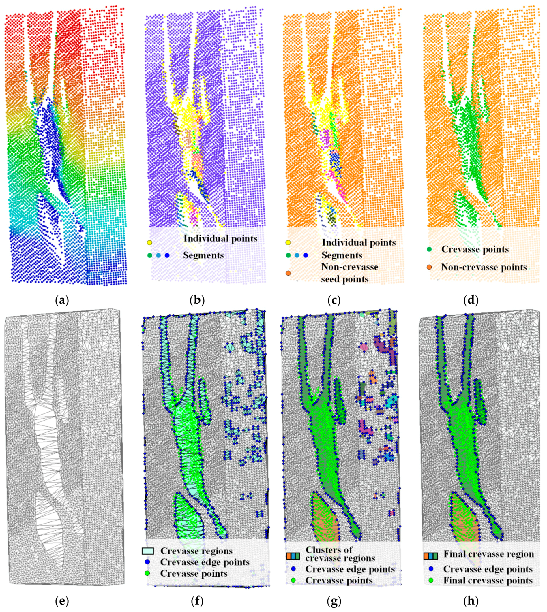
After these three steps, all points are classified as crevasse or non-crevasse. For example, Figure 4a–d is a real case of crevasse points extraction.

3.2. Crevasse Edges/Regions Detection Using a Local Statistical Analysis Method

Although the crevasse points are extracted by the hybrid-entity method, they cannot fully cover a crevasse due to occlusion, water-filled and other factors. The proposed method extracts the crevasse edges by performing a local statistical analysis method based on the spatial distribution of the non-crevasse points, and thus the crevasse regions can be obtained. The main idea is based on the fact that a laser scanner can acquire the non-crevasse points near the crevasse edge, although the crevasse sidewalls and bottom are not measured, and then the non-crevasse points near the crevasse edge can be approximately considered as the edge points of the crevasse.

3.2.1. A Novel Feature: The Longest Triangle Edge Within the One Ring Neighborhood (LTE_ORN)

To extract the approximate crevasse edges, a new feature is designed to distinguish the crevasse edge points from the non-edge points in the non-crevasse points. Generally, a data hole exists in the non-crevasse points within the crevasse region, and non-crevasse points far from the crevasse edge are uniformly distributed within a local area. The distances between the non-edge points and the nearest points in different directions of a horizontal plane are almost equal, and the value is expected to be approximately the point spacing. However, the distances between the crevasse edge point and the nearest non-crevasse points in different directions of a horizontal plane are very divergent, and the maximum value of these distances is larger than the point spacing. Therefore, the proposed method calculates the maximum value of the distances between a point and the nearest points in different directions of a horizontal plane as a novel feature to identify the crevasse edge points.
To simply describe the proximity relationships in different directions of a horizontal plane for each non-crevasse point, without the limitations of the distance and the point density, the proposed method generates a Delaunay triangulation mesh for all non-crevasse points (DTM_NCP), as shown in Figure 4e. Based on the DTM_NCP, the distance of the longest triangle edge (LTE) within the one ring neighborhood (ORN) is taken as the maximum value of the distances between a point and the nearest points in different directions of a horizontal plane, as shown in Figure 5a. From Figure 5a, this approach is an efficient way to describe the differences between crevasse edge points and other non-crevasse points.

3.2.2. Extracting Crevasse Edges Based on an Adaptive Threshold Using DBSCAN

After the calculation of the distance of the LTE_ORN, the approximate crevasse edge points can be extracted by using a threshold ( t L T E ). When the distance of the LTE of a point is larger than t L T E , the point is a crevasse edge point, and the corresponding triangle including the longest edge belongs to the crevasse region. However, the use of a fixed threshold faces a problem. Although the distance of LTE_ORN of a crevasse non-edge point is expected to be approximately equal to the average point spacing, the average point spacing will not be a constant, due to the uneven point density. Therefore, the proposed method calculates an adaptive value for the threshold t L T E using a local statistical analysis method for the set of distances of LTE_ORNs within the neighborhood of each point.
First, the neighboring points of each non-crevasse point are searched using the Kd-tree technique [33], where the radius is set to r , and the LTE_ORNs of the neighboring points comprise the set of L T E s . An example is shown in Figure 5b, the crevasse edge points are assigned with large values, while the distances of L T E s of the non-edge points are smaller and unified. The density-based spatial clustering of applications with noise algorithm (DBSCAN) [37] is then utilized to group the distances of L T E s into several clusters, without the influence of outliers and sample densities, as shown in Figure 5c. The non-edge points generally belong to the first meaningful cluster with the smallest value, while the crevasse edge points can be outliers or belong to the cluster with the larger value. Therefore, the maximum distance of the first cluster is taken as the basic term of the threshold t L T E , as shown in Equation (5). Considering the influence of the point uncertainty and other factors on the distance of the LTE, an error term ( Δ d ) is taken as the second part of the threshold t L T E .
t L T E = d m a x c 1 + Δ d
where t L T E is the adaptive threshold derived by the local statistical method; d m a x c 1 is the maximum value of the first cluster; and Δ d is a value for the error term.
In this way, the adaptive threshold can be obtained for each non-crevasse point, and the proposed method can extract the approximate crevasse edge points, as shown by the blue points in Figure 4f. The triangles that contain the L T E of each approximate crevasse edge point are then extracted as the crevasse triangles, as shown by the cyan triangles in Figure 4f.

3.3. Refining the Crevasse Points/Regions Using a Cross-Analysis Method

Although the crevasse points/edges are efficiently extracted by the hybrid-entity method and the local statistical analysis method, some pseudo-crevasse regions and pseudo-crevasse points will exist. The pseudo-crevasse regions generally exist in the areas of missing data due to the measurement dropouts caused by specular reflection of the laser beam (e.g., a supraglacial river), occlusion, and false triangulation at the border of the study region, as shown in Figure 4f. A few false crevasse points may be erroneously extracted in Section 3.1 due to outliers and some special non-crevasse surface features (e.g., ice cliffs). Therefore, a cross-analysis method is applied to remove pseudo-crevasse regions and pseudo-crevasse points.
(1) Removal of pseudo-crevasse points: Generally, the corresponding crevasse triangles should exist near the extracted crevasse points, and the extracted crevasse points should be lower than the neighboring non-crevasse points. Therefore, the false crevasse points are removed by two steps: (i) If a crevasse point is outside any crevasse triangle, this point is labeled as a pseudo crevasse point and is removed. (ii) If a crevasse edge point lower than the extracted crevasse point, the extracted crevasse point is classified as a pseudo crevasse point.
(2) Removal of pseudo-crevasse regions: Generally, no crevasse points exist in the areas of pseudo-crevasses, and the extracted crevasse points can be taken as the auxiliary data for removing the pseudo-crevasse regions. However, no crevasse points may also exist in some true crevasse triangles within a local area, which may be caused by occlusion, water-filled or the mirror reflection of the crevasse sidewall. In this paper, therefore, false crevasse edges/regions are removed according to the number of corresponding crevasse points on the level of the whole crevasse, which is based on the assumption that existing crevasse points within a whole crevasse is more possible. First, the proposed method groups crevasse triangles into different crevasse regions by the adjacency analysis based on the triangle topology. Figure 4g shows the grouping results for the crevasse triangles. Second, the extracted crevasse points are assigned to each crevasse region. Last, the pseudo-crevasse regions are removed when the number of crevasse points is smaller than the threshold t n (e.g., five).
After removing the pseudo-crevasse points and regions, the final crevasse points and regions are extracted. For example, Figure 4h displays the final result of the crevasse detection for the real case.

4. Results and Performance Analysis

4.1. Experimental Results

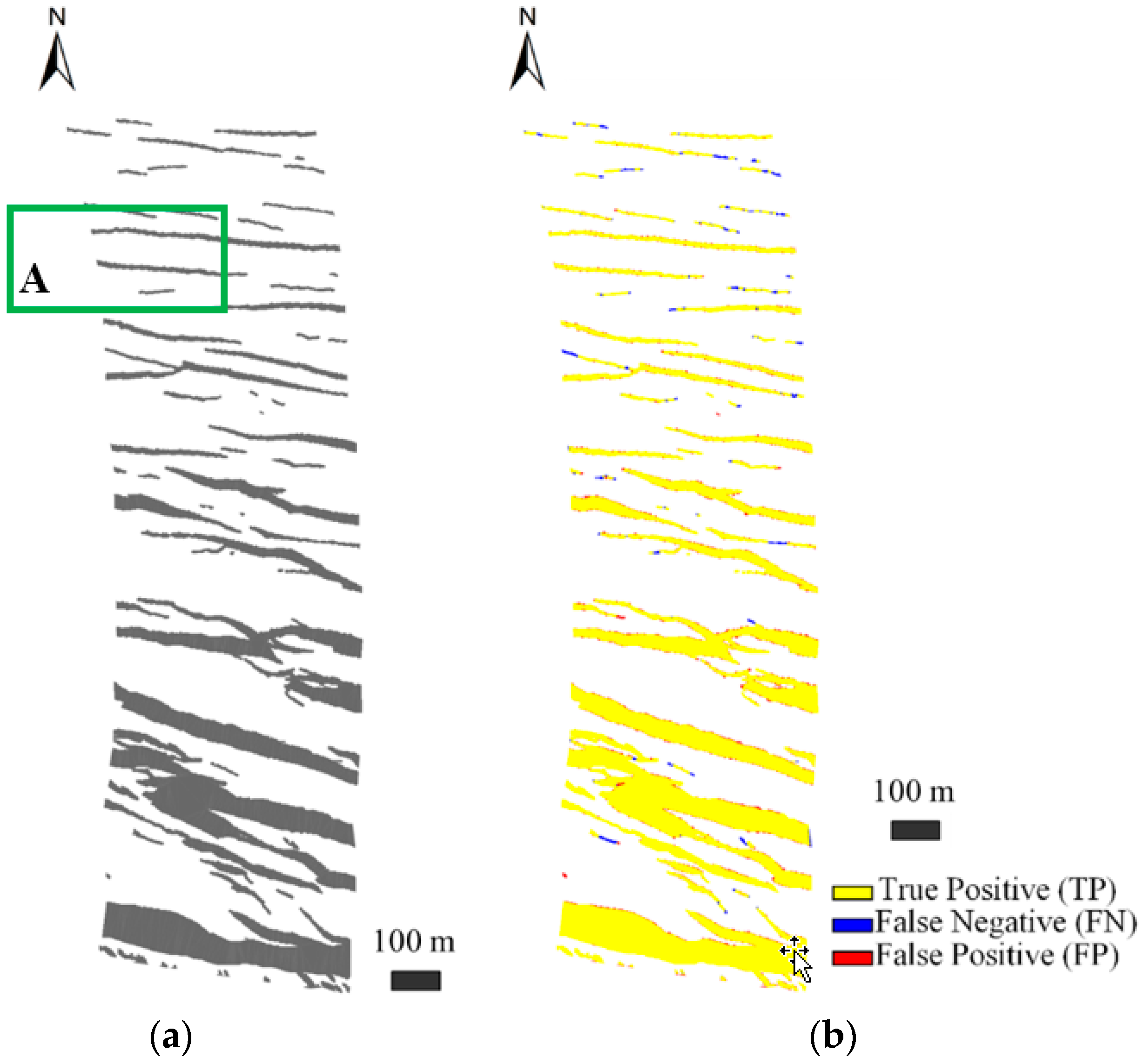
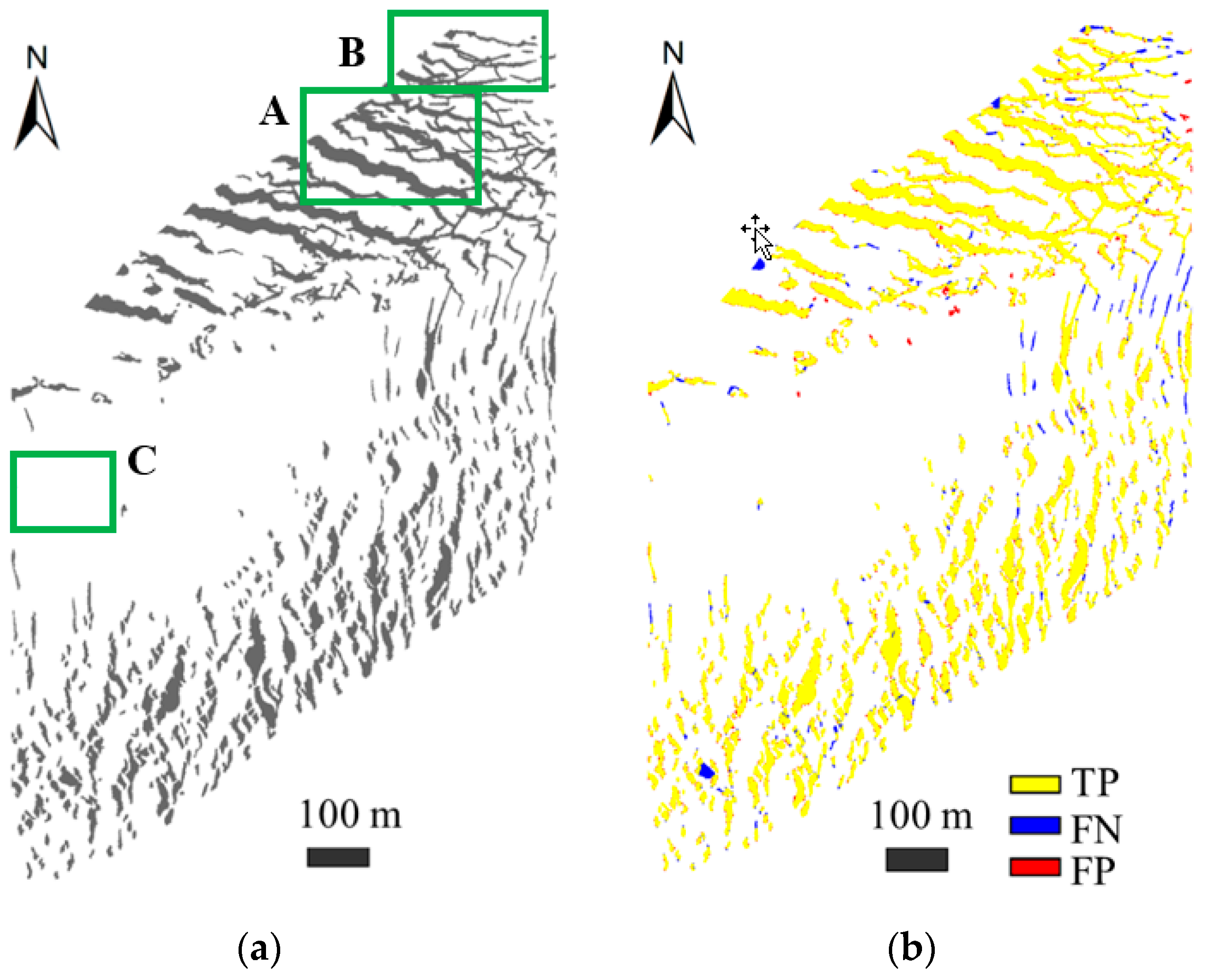
The proposed method was utilized to extract crevasses from the point clouds of the two sites, using the parameter settings listed in Table 2. The results are shown in Figure 6a and Figure 7a.
To evaluate the performance of the proposed method, the region of each crevasse with a width larger than the point spacing was manually delineated as the reference. The differences and overlaps of the extracted crevasse regions and the reference crevasse regions were determined. The evaluation results are shown in Figure 6b and Figure 7b. The evaluation results were quantitatively calculated by employing three indices: Recall ( R ), Precision ( P ), and the F 1 score. These three indices are defined in Equations (6)–(8), respectively. The quantitative evaluation results are listed in Table 3, which shows that the proposed method achieves excellent results, with high values of R , P , and F 1 . All three indices on the two sites are larger than 94.00%. The R value of the first site is the best: 98.42%.
P = T P T P + F P × 100 %
R = T P T P + F N × 100 %
F 1 = 2 · R · P P + R × 100 %
where R is the recall index; P denotes the precision index; T P is the area of correctly detected crevasse regions; F P is the area of erroneously detected crevasse regions; and F N is the area of erroneously removed crevasse regions. F 1 is a measure that combines precision and recall.
As shown in Figure 6b and Figure 7b, and Table 3, most of the crevasses have been correctly extracted. Only a few crevasses have been lost, and a few non-crevasse regions are falsely classified as crevasse regions.

4.2. Performance Analysis of the Proposed Method

In this part, first, the influence of the parameter settings on the crevasse detection results were analyzed. Second, the importance of the horizontal analysis was evaluated. Last, the proposed method was compared with a morphological method based on the DEM derived from LiDAR point clouds. The second site (i.e., Site 2) was considered with a complex glacier surface as the experimental data.

4.2.1. Parameter Sensitivity Analysis

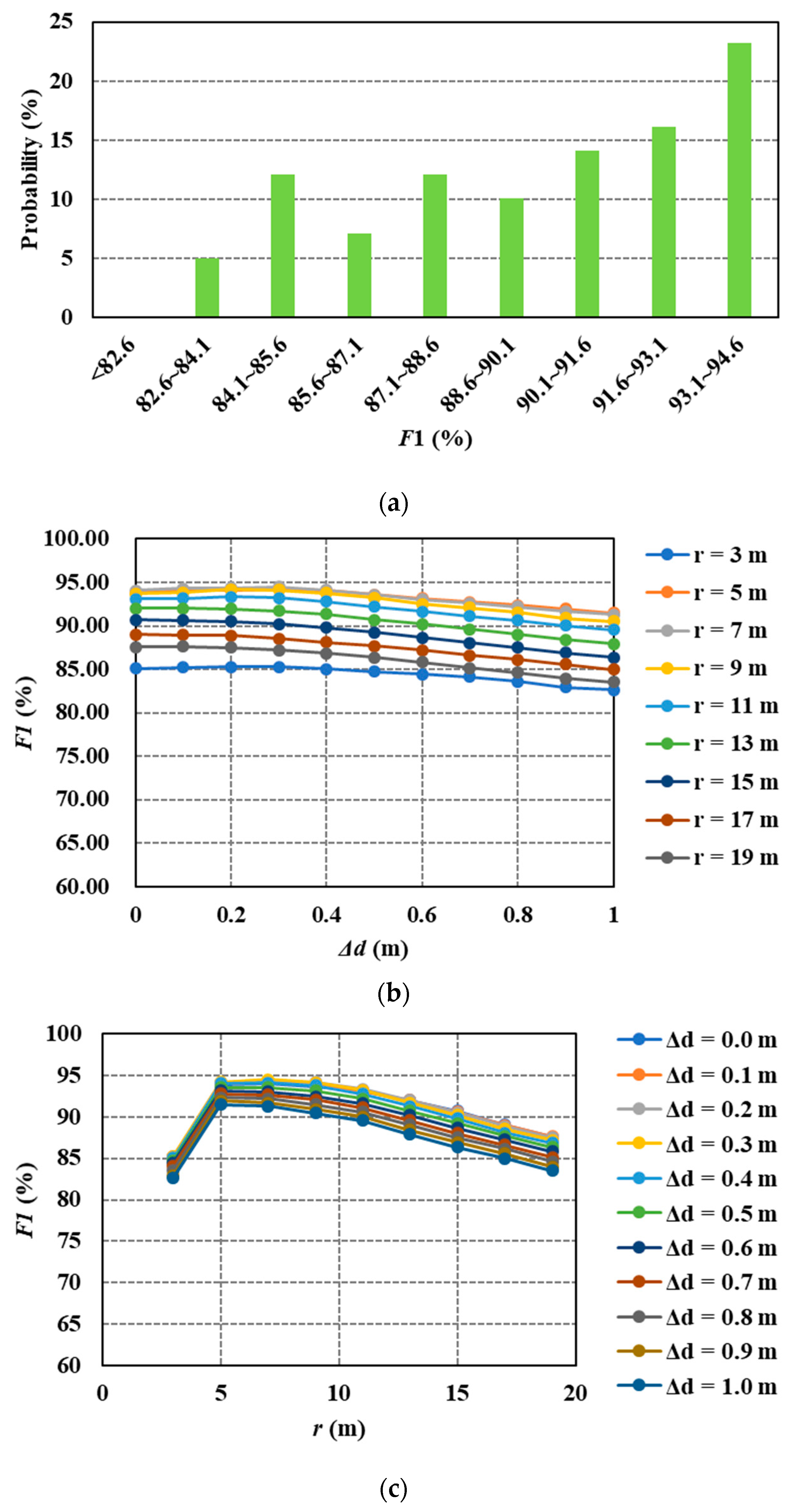
To evaluate the robustness of the proposed method, experiments with different parameter configurations were performed. As the horizontal analysis is the most important contribution of the proposed method, the two related parameters (i.e., Δ d and r ) were chosen for the analysis. Parameter r varied from 3.0 m to 19.0 m, with an interval of 2.0 m, and parameter Δ d varied from 0.0 m to 1.0 m, with an interval of 0.1 m. A total of 99 configurations existed. The histogram of the results is plotted in Figure 8a, where the number of bars was set to eight. The F 1 score is larger than 90.00% for 55% of all parameter configurations. However, the difference between the minimum F 1 score and the maximum F 1 score is large—more than 10.00%. To further establish the influence of the change in each parameter on the crevasse detection, independent analyses for Δ d and r were performed. The corresponding results are shown in Figure 8b,c. As shown in Figure 8b, the influence of Δ d is moderate. The maximum F 1 score difference of nine curves is approximately 4.5%. The F 1 score difference between Δ d = 0.0   m and Δ d = 0.3   m is very small, and the maximum F 1 score difference of nine curves is only 0.52%. However, the influence of r is greater than that of Δ d . As shown in Figure 8c, the maximum F 1 scores achieved are between r = 5.0   m and r = 7.0   m , and the F 1 score difference between r = 5.0   m and r = 7.0   m is less than 0.28% for eleven curves of different values for Δ d . The curves have sudden and increasing changes from r = 3.0   m to r = 5.0   m , and the maximum F 1 score difference is 9.02%. When r is larger than 5.0 m, the curve shows a slow downward trend, with an average slope of ~30°. The main reason is that the adaptive threshold in the process of the horizontal analysis cannot be correctly obtained when the neighborhood size is too large or too small. In summary, the proposed method is relatively robust when the two parameters are set to values within reasonable ranges.

4.2.2. The Importance Evaluation of the Horizontal Analysis

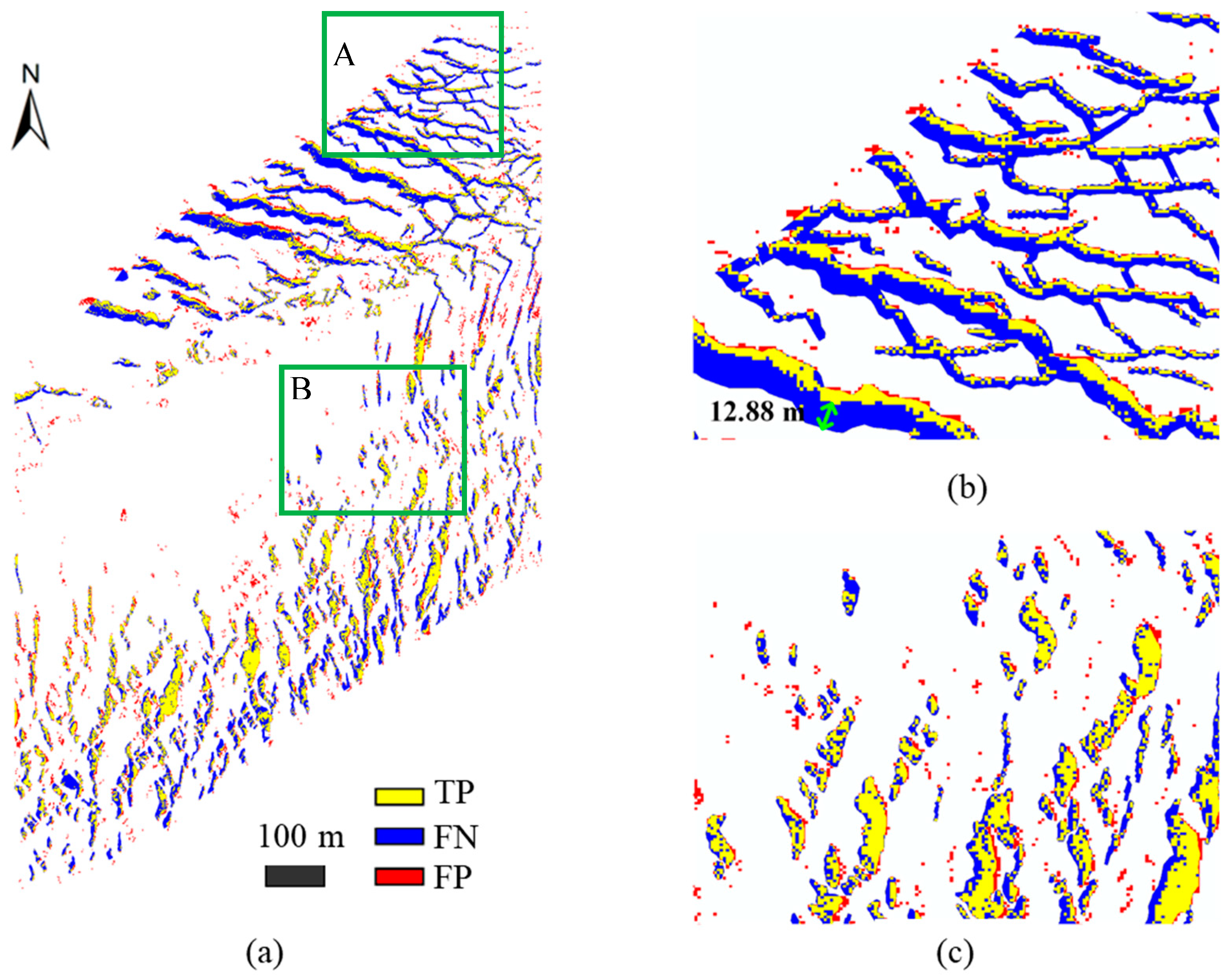
To evaluate the importance of the horizontal analysis for obtaining more complete crevasse regions from the occlusion point clouds, the proposed method was compared with the crevasse point detection result which only includes Section 3.1. The evaluation result of crevasse point detection is plotted in Figure 9a. It is observed that most of crevasse regions are lost in the result due to the occlusion and water-filled, and some commission pixels are caused by outliers and other factors, as shown in Figure 9b,c. Statistically, the recall of the crevasse points detection is 41.49%, which is substantially less than the recall of the proposed method. As shown in Figure 9b, many omission regions exist around the crevasse edges, where the width of the crevasse region without points is larger than 12.0 m at the green arrow. In this way, the width of a crevasse cannot be correctly obtained by the crevasse points detection but can be calculated from the crevasse edges derived by the horizontal analysis. This finding demonstrates that the horizontal analysis is important.

4.2.3. Comparison with a Morphological Method Based on the LiDAR DEM

In this part, the proposed method was compared with a morphological method based on the LiDAR DEM, where the crevasse pixels are detected by using an operator of Black Top Hat [38] with a height difference threshold (i.e., 0.5 m). To overcome the influence of the interpolation method and the number of scales in the morphological method, three interpolation methods (i.e., inverse distance weighted (IDW), triangulated irregular network (TIN) and nearest neighbor (NN)) were chosen for generating the DEMs, and two versions of the morphological methods (i.e., the single-scale morphological method and multi-scale morphological method) were performed. In this way, six results, which are listed in Table 4, were derived. All the results show that the F 1 of the six results are small, where the largest value is 73.90% and the smallest value is 61.76%. The comparison of the six results indicates that the combination of the TIN interpolation method and the multi-scale morphological method is the best. However, many more errors around the crevasse edges exist in the results based on DEM interpolated by IDW and NN, and many more undulating non-crevasse glacier surfaces are mistaken as the crevasse by the single scale morphological method. It is because: (a) The TIN interpolation method can implicitly express the breaklines between the crevasse and non-crevasse to avoid the obvious errors of crevasse edges in other interpolation methods; (b) the multi-scale morphological method can partly reduce the influence of the undulating non-crevasse surfaces.
Compared with the result of the proposed method, the best of the six results are substantially worse in this scene with a complex glacier surface. The main reasons are also two-fold: (a) The best precision of six results is only 67.44%, which is much smaller than that of the proposed method; (b) in the six results, the maximum value of the recall is 85.14%, which is smaller than that of the proposed method with 9.69%.

5. Discussion

5.1. Advantages and Limitations of the Proposed Method

In this part, the advantages and limitations of the proposed method are discussed. Firstly, excellent performance may be attributed to the following aspects:
1. The whole of a crevasse can be better detected by combining vertical and horizontal analysis. For example, two cases are shown in Figure 10. Figure 10a shows that the proposed method can detect the whole region of a crevasse when part of a crevasse is not measured. Another case is shown in Figure 10b. Although the small crevasses have only sparse crevasse points with discontinuous spatial distributions, the proposed method can also detect the crevasse regions.
2. The proposed method can remove the pseudo-crevasse points and regions by a cross-analysis method. For example, Figure 11a is a non-crevasse region with data holes, which is located in rectangle B of Figure 7. In this region, the loss of returns of many laser beams may have been synthetically caused by the large incident angles near the border of the scanning swath, the over-smooth glacier surface, and other factors. These issues enable the detection of a pseudo-crevasse region in the processing of the horizontal analysis, as shown in Figure 11b,c shows the final result. The pseudo-crevasse regions can be removed by the help of the extracted crevasse points.
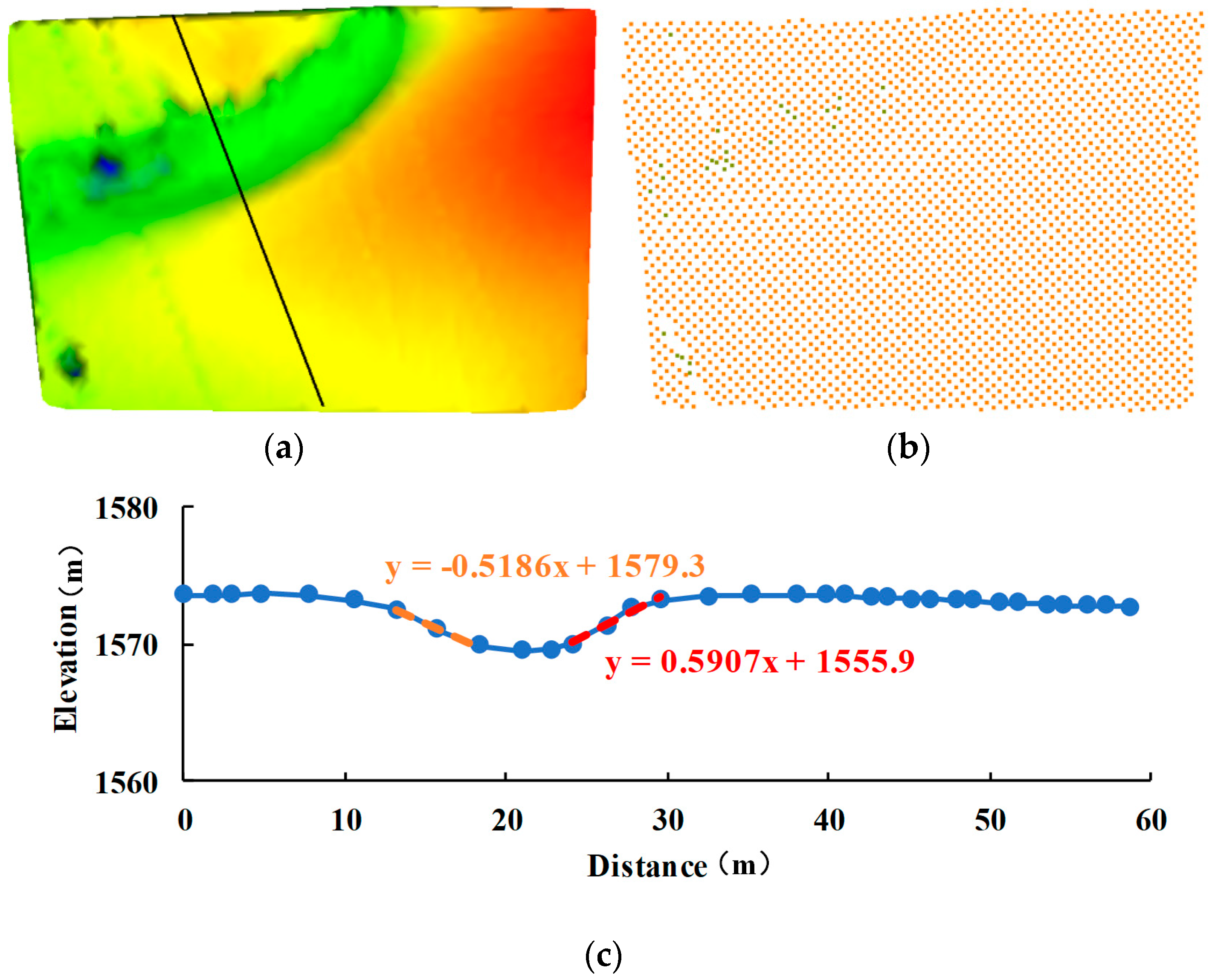
3. The proposed method can overcome the influence of the undulating glacier surface within the non-crevasse region. The main reasons are two-fold: (a) The proposed method employs the segment entities to connect the neighboring points with a smooth elevation change; (b) an assumption of nearly vertical crevasse sidewalls is made. For example, Figure 12 is a region with a greatly undulating glacier surface. From Figure 12c, the elevation difference of the concave surface exceeds 4 m. However, the slopes of the two sides of the concave surface are small. The slope values are only 27.4° and 30.6°, respectively. According to the law of a crevasse, the sidewall of a crevasse is nearly vertical, which shows the concave surface is not a crevasse. Figure 12b depicts the result of separating crevasse points from non-crevasse points using the proposed method. All points are almost classified into non-crevasse points, and no pseudo-crevasse regions are detected.
4. The proposed method can achieve excellent results in regions with different point densities. As shown in the evaluation result for Site 2 in Figure 7b, the quality of the result is excellent in the overlapping region of the two strips with a high point density and the border region of a single strip with a low point density.
Although the results for the study sites are excellent, a few errors occurred in the results. On the one hand, the quality of the crevasse regions detection is severely affected by the point density. In the process of the horizontal analysis, the crevasse regions are extracted by an adaptive threshold derived by the local statistical analysis method, which assumes that the width of a crevasse is larger than the point spacing of the neighboring non-crevasse point. However, a very small crevasse cannot be detected when its width is not distinctly larger than the scanning point spacing. Moreover, the omission errors may be caused by other factors, including crevasses covered by snow. These problems can be overcome in future research by fusing very high-resolution images and other remote sensing data. On the other hand, it may fail to remove supraglacial rivers in the refining process, when supraglacial rivers are linked to crevasses or some pseudo crevasse points are mistakenly detected in the regions of supraglacial rivers. To robustly remove supraglacial rivers, attempts will be made to perform the analysis of strain rate change in the detected crevasse regions [39].

5.2. Potential of the Crevasse Detection Result in the Estimation of the Crevasse Depth

Airborne LiDAR can directly acquire the three-dimension information of the crevasse, and it could be considered as a manner to derive the crevasse depth on a large scale. When the crevasse is fully measured, including the crevasse bottom, the crevasse depth can be easily measured using the extracted crevasse points. However, most crevasses cannot be fully measured. Only part of the crevasse sidewalls can be acquired, and the crevasse bottom is difficult to be covered. The depth was generally derived by using fitting methods based on some assumptions (e.g., V-shaped crevasses) [12,22], which replaces direct measuring. However, the assumptions are difficult to be made for the complex shape of the crevasse. In the literature [40], Enderlin and Bartholomaus extracted crevasses from the Airborne LiDAR elevation profile using the local elevation minimum and maximum, and the crevasse depth is then derived by the linear fitting of the crevasse sidewall. However, the directions of crevasses are various, the elevation profiles may be not perpendicular to all related crevasses, and the precision of the derived depth is affected. In this paper, the point clouds acquired by ALS were used. Most of the crevasse information could be obtained except for the occlusion and water-filled areas. The proposed method automatically extracted crevasse points and edges. That is to say, the horizontal spatial extent of each crevasse was completely achieved by the proposed method, and the three-dimensional data of crevasse sidewalls and bottom can be partly or completely obtained. In this way, the centerline of each crevasse can be delineated, and the crevasse depth can be better fitted based on the points of the crevasse within a rectangle perpendicular to the crevasse centerline, where the extracted crevasse edges can be also taken as the boundary conditions simultaneously. Moreover, for the derived depth, its uncertainty is synthetically decided by the shape of the crevasse, the degree of coverage of crevasse points on the crevasse sidewalls, the precision of laser scanning and other factors. Estimating the value is difficult using the error model. Due to a lack of field measurements, estimating the uncertainty by the validating data is also difficult at present. Therefore, performing the simultaneous observation of the crevasse using the ALS and the field measurements will be necessary in the future. In a word, the potential of deriving the crevasse depth from the detected crevasse points and edges is satisfactory despite several difficulties.

6. Conclusions

This paper proposed a bidirectional analysis method to obtain three-dimensional glacier crevasses from Airborne LiDAR point clouds, where the vertical and horizontal characteristics of crevasses are employed. The proposed method robustly separates crevasse points from non-crevasse points according to the elevation of a crevasse point, which is lower than that of the neighboring non-crevasse points, and the nearly vertical characteristic of the crevasse sidewall. The proposed method detects the crevasse edges and regions by the use of a novel feature (i.e., the longest triangle edge within the one ring neighborhood), based on the Delaunay triangulation network of non-crevasse points, to overcome the influence of the occlusion and water-filled.
Two airborne LiDAR datasets from two sites of Alaskan glaciers (i.e., Tyndall Glacier and Seward Glacier) were selected to evaluate the performance of the proposed method. The experiments showed that the proposed method can achieve excellent results, with the F 1 scores of both sites being more than 94.00%. The Tyndall site with a complex glacier surface was then used as a case study to investigate the robustness of the proposed method and to evaluate the importance of the horizontal analysis and to compare the proposed method with a morphological method of crevasse detection from the LiDAR DEM. The results confirmed that: (a) The proposed method is robust when the key parameters are set to values within reasonable ranges; (b) the horizontal analysis can obtain the crevasse edges as the complementary data for obtaining more complete crevasses; (c) the performance of the proposed method is substantially better than the morphological method. Moreover, the proposed method was discussed from two aspects: The advantages and limitations of the proposed method, and the potential of the results of the proposed method in the retrieval of the crevasse depth.
In our future works, attempts will be made to solve the existing problems in the proposed method (e.g., snow bridges and removal of supraglacial rivers). Moreover, the authors intend to study the methods for deriving the three-dimensional parameters of crevasses (e.g., the width, depth, and direction) from the crevasse detection result, and build the time series to analyze their spatio-temporal variation characteristics and the corresponding reasons.

Author Contributions

The methodology was designed by R.H., L.J., H.W., and B.Y.; and the manuscript was written by R.H. and L.J.

Funding

This research was funded by the National Key R&D Program of China (Nos. 2018YFC1406102 and 2017YFA0603103); the China Postdoctoral Science Fund (No. 2017M622553 and 2019T120695); the NSFC project (Nos. 41801398); the Key Research Program of Frontier Sciences, CAS (Nos. QYZDB-SSW-DQC027, QYZDJ-SSW-DQC042); and the Strategic Priority Research Program of the Chinese Academy of Sciences (No. XDA19070104).

Acknowledgments

The authors would like to thank National Snow & Ice Data Center for providing the lidar data. The authors are very grateful to the anonymous reviewers for their helpful suggestions.

Conflicts of Interest

The authors declare no conflict of interest.

References

  1. Vaughan, D.G. Relating the occurrence of crevasses to surface strain rates. J. Glaciol. 1993, 39, 255–266. [Google Scholar] [CrossRef] [Green Version]
  2. Campbell, S.; Roy, S.; Kreutz, K.; Arcone, S.A.; Osterberg, E.C.; Koons, P. Strain-rate estimates for crevasse formation at an alpine ice divide: Mount Hunter, Alaska. Ann. Glaciol. 2013, 54, 200–208. [Google Scholar] [CrossRef] [Green Version]
  3. Colgan, W.; Steffen, K.; McLamb, W.S.; Abdalati, W.; Rajaram, H.; Motyka, R.; Phillips, T.; Anderson, R. An increase in crevasse extent, West Greenland: Hydrologic implications. Geophys. Res. Lett. 2011, 38, L18502. [Google Scholar] [CrossRef]
  4. Fountain, A.G.; Jacobel, R.W.; Schlichting, R.; Jansson, P. Fractures as the main pathways of water flow in temperate glaciers. Nature 2005, 433, 618–620. [Google Scholar] [CrossRef] [PubMed]
  5. Benn, D.; Gulley, J.; Luckman, A.; Adamek, A.; Glowacki, P.S. Englacial drainage systems formed by hydrologically driven crevasse propagation. J. Glaciol. 2009, 55, 513–523. [Google Scholar] [CrossRef] [Green Version]
  6. Das, S.B.; Joughin, I.; Behn, M.D.; Howat, I.M.; King, M.A.; Lizarralde, D.; Bhatia, M.P. Fracture propagation to the base of the Greenland Ice Sheet during supraglacial lake drainage. Science 2008, 320, 778–781. [Google Scholar] [CrossRef] [PubMed]
  7. Mottram, R.H.; Benn, D.I. Testing crevasse-depth models: A field study at Breiðamerkurjökull, Iceland. J. Glaciol. 2009, 55, 746–752. [Google Scholar] [CrossRef]
  8. Benn, D.I.; Warren, C.R.; Mottram, R.H. Calving processes and the dynamics of calving glaciers. Earth-Sci. Rev. 2007, 82, 143–179. [Google Scholar] [CrossRef]
  9. Colgan, W.; Rajaram, H.; Abdalati, W.; McCutchan, C.; Mottram, R.; Moussavi, M.S.; Grigsby, S. Glacier crevasses: Observations, models, and mass balance implications. Rev. Geophys. 2016, 54, 119–161. [Google Scholar] [CrossRef]
  10. Bhardwaj, A.; Sam, L.; Bhardwaj, A.; Javier Martin-Torres, F. LiDAR remote sensing of the cryosphere: Present applications and future prospects. Remote Sens. Environ. 2016, 177, 125–143. [Google Scholar] [CrossRef]
  11. Fricker, H.A. Multi-year monitoring of rift propagation on the Amery Ice Shelf, East Antarctica. Geophys. Res. Lett. 2005, 32. [Google Scholar] [CrossRef] [Green Version]
  12. Liu, Y.; Cheng, X.; Hui, F.; Wang, X.; Wang, F.; Cheng, C. Detection of crevasses over polar ice shelves using Satellite Laser Altimeter. Sci. China Earth Sci. 2014, 57, 1267–1277. [Google Scholar] [CrossRef]
  13. Bhardwaj, A.; Sam, L.; Singh, S.; Kumar, R. Automated detection and temporal monitoring of crevasses using remote sensing and their implications for glacier dynamics. Ann. Glaciol. 2016, 57, 81–91. [Google Scholar] [CrossRef] [Green Version]
  14. Dall’Asta, E.; Forlani, G.; Roncella, R.; Santise, M.; Diotri, F.; Morra di Cella, U. Unmanned Aerial Systems and DSM matching for rock glacier monitoring. ISPRS J. Photogramm. Remote Sens. 2017, 127, 102–114. [Google Scholar] [CrossRef]
  15. Kääb, A. Monitoring high-mountain terrain deformation from repeated air- and spaceborne optical data: Examples using digital aerial imagery and ASTER data. ISPRS J. Photogramm. Remote Sens. 2002, 57, 39–52. [Google Scholar] [CrossRef]
  16. Pieczonka, T.; Bolch, T.; Buchroithner, M. Generation and evaluation of multitemporal digital terrain models of the Mt. Everest area from different optical sensors. ISPRS J. Photogramm. Remote Sens. 2011, 66, 927–940. [Google Scholar] [CrossRef]
  17. Shean, D.E.; Alexandrov, O.; Moratto, Z.M.; Smith, B.E.; Joughin, I.R.; Porter, C.; Morin, P. An automated, open-source pipeline for mass production of digital elevation models (DEMs) from very-high-resolution commercial stereo satellite imagery. ISPRS J. Photogramm. Remote Sens. 2016, 116, 101–117. [Google Scholar] [CrossRef] [Green Version]
  18. Li, R.; Xiao, H.; Liu, S.; Tong, X. A Systematic Study of the Fracturing of Ronne—Filchner Ice Shelf, Antarctica, Using Multisource Satellite Data from 2001 to 2016. Cryosphere Discuss. 2017. [Google Scholar] [CrossRef]
  19. Ryan, J.C.; Hubbard, A.L.; Box, J.E.; Todd, J.; Christoffersen, P.; Carr, J.R.; Holt, T.O.; Snooke, N. UAV photogrammetry and structure from motion to assess calving dynamics at Store Glacier, a large outlet draining the Greenland ice sheet. Cryosphere 2015, 9, 1–11. [Google Scholar] [CrossRef] [Green Version]
  20. Höfle, B.; Geist, T.; Rutzinger, M.; Pfeifer, N. Glacier surface segmentation using airborne laser scanning point cloud and intensity data. Int. Arch. Photogramm. Remote Sens. Spat. Inf. Sci. 2007, 36 Pt 3, W52. [Google Scholar]
  21. Fritzmann, P.; Höfle, B.; Vetter, M.; Sailer, R.; Stötter, J.; Bollmann, E. Surface classification based on multi-temporal airborne LiDAR intensity data in high mountain environments: A case study from Hintereisferner, Austria. Z. Geomorphol. Suppl. Issues 2011, 55, 105–126. [Google Scholar] [CrossRef]
  22. Kodde, M.; Pfeifer, N.; Gorte, B.; Geist, T.; Höfle, B. Automatic glacier surface analysis from airborne laser scanning. Int. Arch. Photogramm. Remote Sens. Spat. Inf. Sci. 2007, 36 Pt 3, 221–226. [Google Scholar]
  23. Yang, B.; Huang, R.; Dong, Z.; Zang, Y.; Li, J. Two-step adaptive extraction method for ground points and breaklines from lidar point clouds. ISPRS J. Photogramm. Remote Sens. 2016, 119, 373–389. [Google Scholar] [CrossRef]
  24. Foroutan, M.; Marshall, S.J.; Menounos, B. Automatic mapping and geomorphometry extraction technique for crevasses in geodetic mass-balance calculations at Haig Glacier, Canadian Rockies. J. Glaciol. 2019, 1–12. [Google Scholar] [CrossRef]
  25. Telling, J.; Glennie, C.; Fountain, A.; Finnegan, D. Analyzing glacier surface motion using LiDAR data. Remote Sens. 2017, 9, 283. [Google Scholar] [CrossRef]
  26. Arnold, N.; Rees, W.; Devereux, B.; Amable, G. Evaluating the potential of high-resolution airborne LiDAR data in glaciology. Int. J. Remote Sens. 2006, 27, 1233–1251. [Google Scholar] [CrossRef]
  27. Li, J.; Yang, B.; Cong, Y.; Cao, L.; Fu, X.; Dong, Z. 3D Forest Mapping Using A Low-Cost UAV Laser Scanning System: Investigation and Comparison. Remote Sens. 2019, 11, 717. [Google Scholar] [CrossRef]
  28. Johannesson, T.; Bjornsson, H.; Palsson, F.; Sigurdsson, O.; Porsteinsson, P. LiDAR mapping of the Snaefellsjokull ice cap, western Iceland. Jokull 2011, 61, 19–32. [Google Scholar]
  29. Larsen, C. IceBridge UAF Lidar Scanner L1B Geolocated Surface Elevation Triplets, Version 1; NASA National Snow and Ice Data Center Distributed Active Archive Center: Boulder, CO, USA, 2018.
  30. Van der Veen, C. Crevasses on glaciers. Polar Geogr. 1999, 23, 213–245. [Google Scholar] [CrossRef]
  31. Vosselman, G.; Coenen, M.; Rottensteiner, F. Contextual segment-based classification of airborne laser scanner data. ISPRS J. Photogramm. Remote Sens. 2017, 128, 354–371. [Google Scholar] [CrossRef]
  32. Huang, R.; Jiang, L.; Shen, X.; Dong, Z.; Zhou, Q.; Yang, B.; Wang, H. An efficient method of monitoring slow-moving landslides with long-range terrestrial laser scanning: A case study of the Dashu landslide in the Three Gorges Reservoir Region, China. Landslides 2019, 16, 839–855. [Google Scholar] [CrossRef]
  33. Yang, B.; Dong, Z.; Liu, Y.; Liang, F.; Wang, Y. Computing multiple aggregation levels and contextual features for road facilities recognition using mobile laser scanning data. ISPRS J. Photogramm. Remote Sens. 2017, 126, 180–194. [Google Scholar] [CrossRef]
  34. Huang, R.; Yang, B.; Liang, F.; Dai, W.; Li, J.; Tian, M.; Xu, W. A top-down strategy for buildings extraction from complex urban scenes using airborne LiDAR point clouds. Infrared Phys. Technol. 2018, 92, 203–218. [Google Scholar] [CrossRef]
  35. Tóvári, D.; Pfeifer, N. Segmentation based robust interpolation-a new approach to laser data filtering. Int. Arch. Photogramm. Remote Sens. Spat. Inf. Sci. 2005, 36, 79–84. [Google Scholar]
  36. Edelsbrunner, H.; Mücke, E.P. Three-dimensional alpha shapes. ACM Trans. Graph. (TOG) 1994, 13, 43–72. [Google Scholar] [CrossRef]
  37. Ester, M.; Kriegel, H.-P.; Sander, J.; Xu, X. A density-based algorithm for discovering clusters in large spatial databases with noise. In Proceedings of the International Conference on Knowledge Discovery and Data Mining (KDD96), Portland, OR, USA, 2–4 August 1996; pp. 226–231. [Google Scholar]
  38. Rodriguez, F.; Maire, E.; Courjault-Rade, P.; Darrozes, J. The Black Top Hat function applied to a DEM: A tool to estimate recent incision in a mountainous watershed (Estibere Watershed, Central Pyrenees). Geophys. Res. Lett. 2002, 29, 9-1–9-4. [Google Scholar] [CrossRef]
  39. Emetc, V.; Tregoning, P.; Morlighem, M.; Borstad, C.; Sambridge, M. A statistical fracture model for Antarctic ice shelves and glaciers. The Cryosphere 2018, 12, 3187–3213. [Google Scholar] [CrossRef] [Green Version]
  40. Enderlin, E.M.; Bartholomaus, T.C. Poor performance of a common crevasse model at marine-terminating glaciers. The Cryosphere Discuss. 2019, 1–19. [Google Scholar] [CrossRef] [Green Version]
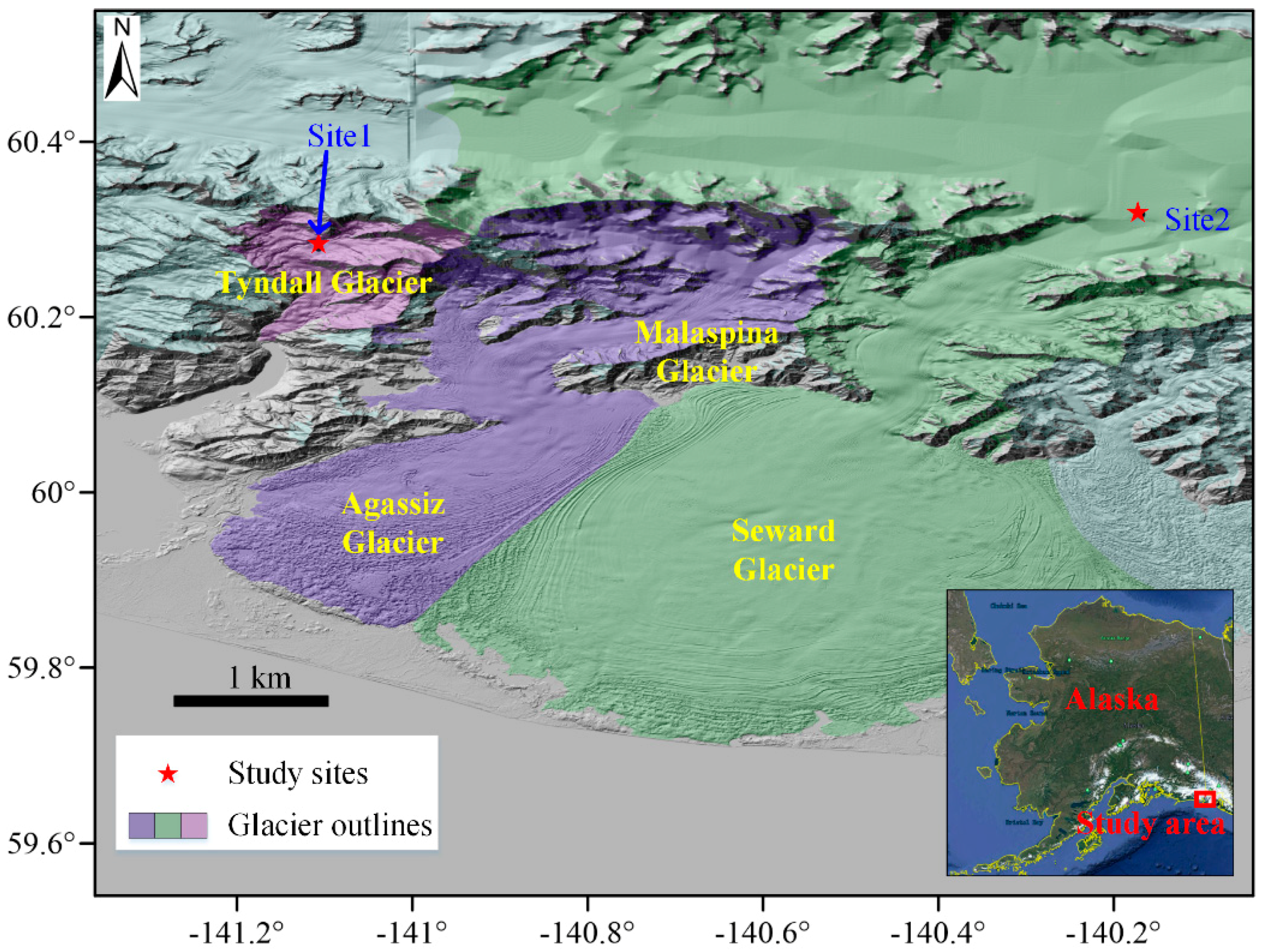
Figure 1. Locations of the study sites. Glacier outlines originate from the Randolph Glacier Inventory (RGI 6.0) (https://www.glims.org/RGI/rgi60_dl.html).
Remotesensing 11 02373 g001
Figure 2. Point clouds of the two sites. (a) Point clouds of the first site. (b) Point clouds of the second site. (c) Profile of Pa in subgraph (a). (d) Profile of Pb in subgraph (b).
Remotesensing 11 02373 g002
Figure 3. Workflow of the proposed bidirectional analysis method.
Remotesensing 11 02373 g003
Figure 4. A real case for extracting crevasse points and edges. (a) Raw point cloud. (b) Representation of the point cloud based on the hybrid entities. (c) Extraction of the non-crevasse seed points. (d) Result of crevasse points extraction. (e) Generated Delaunay triangulation mesh of non-crevasse points. (f) Initial crevasse regions, crevasse edge points, and crevasse points. (g) Result of grouping the crevasse triangles. (h) Result of refining the extracted crevasse regions and points.
Remotesensing 11 02373 g004
Figure 5. Illustration of the process of calculating the adaptive distance threshold using the DBSCAN algorithm. (a) Obtaining the longest triangle edge (LTE) within the one ring neighborhood (ORN) for a point of interest (POI). (b) Spatial distribution of the distances of the LTEs within a local neighborhood. (c) Grouping the distances of the LTEs within a local neighborhood of the POI by DBSCAN. (d) Calculating the adaptive threshold based on the grouping result of (c).
Remotesensing 11 02373 g005
Figure 6. Extracted crevasses for Site 1 and quality evaluation. (a) Result of the detected crevasse regions. (b) Evaluation result for the crevasse region detection.
Remotesensing 11 02373 g006
Figure 7. Extracted crevasses for Site 2 and quality evaluation. (a) Result of the detected crevasse regions. (b) Evaluation result for the crevasse region detection.
Remotesensing 11 02373 g007
Figure 8. Analysis of the influence of parameter settings on the crevasse detection. (a) Histogram of the crevasse detection results based on different configurations of Δ d and r . (b) Independent analysis of the influence of Δ d on crevasse detection. (c) Independent analysis of the influence of r on crevasse detection.
Remotesensing 11 02373 g008
Figure 9. Evaluation result of the crevasse point extraction. (a) Evaluation result. (b) Local view of rectangle A in subgraph (a). (c) Local view of the rectangle B in subgraph (a).
Remotesensing 11 02373 g009
Figure 10. Local views of the extracted crevasses in two cases. (a) Extracted crevasse regions and points of rectangle A of Figure 7, where crevasse points are only located at one side of a crevasse. (b) Extracted crevasse regions and points of rectangle A of Figure 6 for small crevasses with sparse and discontinuous crevasse points.
Remotesensing 11 02373 g010
Figure 11. Local view of a case with data holes within rectangle B of Figure 7. (a) Classified point clouds, where many data holes exist on the non-crevasse surfaces. (b) Extracted crevasse points and crevasse regions before refining. (c) Final result of crevasse extraction.
Remotesensing 11 02373 g011
Figure 12. A case of crevasse detection in rectangle C of Figure 7 with an undulating glacier surface. (a) DEM. (b) Crevasse points detection result. (c) Relationship graph between the distance and the elevation for the profile in subgraph (a).
Remotesensing 11 02373 g012
Table 1. General configuration of the University of Alaska Fairbanks (UAF) flight campaigns.
ItemValue
Scanning systemRiegl LMS-Q240i
Laser wavelength905 nm
Height above ground (HAG)500–600 m
Footprint size~20 cm
Horizontal and vertical accuracies of points±30 cm
Pulse repetition frequency20 kHz
Average point spacing~1 m
Table 2. Main parameters settings for the proposed method.
ParameterValueDescription
T d 30.0 mThe neighborhood size for obtainding non-crevasse seed points.
T h 0.5 mThe height threshold for extracting individual crevasse points.
T α 45.0°The angle threshold for describing the vertical or near-vertical crevasse sidewalls.
r 8.0 mThe neighborhood size for the local statistical analysis.
Δ d 0.3 mThe error term of the adaptive distance threshold.
t n 5To remove the pseudo crevasse regions using the corresponding crevasse points.
Table 3. Performance evaluation of the proposed method for the two sites.
TP/m2FP/m2FN/m2Recall/%Precision/%F1/%
Site 149,058.31778.5787.398.4296.5097.45
Site 287,550.75191.44774.894.8394.4094.61
Table 4. Performance evaluation for the morphological method at Site 2.
Interpolation MethodExtraction MethodTP/m2FP/m2FN/m2Recall/%Precision/%F1/%
IDWSS77,425.756,009.414,899.883.8658.0268.59
MS72,429.437,956.219,896.178.4565.6171.46
TINSS78,605.150,786.313,720.485.1460.7570.91
MS75,446.536,427.116,879.081.7267.4473.90
NNSS63,265.649,280.129,059.968.5256.2161.76
MS59,616.633,434.732,708.964.5764.0764.32
Notes. SS and MS denote the single scale morphological method and multi-scale morphological method respectively.