Geometric Characterization of Vines from 3D Point Clouds Obtained with Laser Scanner Systems

Abstract

The 3D digital characterization of vegetation is a growing practice in the agronomy sector. Precision agriculture is sustained, among other methods, by variables that remote sensing techniques can digitize. At present, laser scanners make it possible to digitize three-dimensional crop geometry in the form of point clouds. In this work, we developed several methods for calculating the volume of vine wood, with the final intention of using these values as indicators of vegetative vigor on a thematic map. For this, we used a static terrestrial laser scanner (TLS), a mobile scanning system (MMS), and six algorithms that were implemented and adapted to the data captured and to the proposed objective. The results show that, with TLS equipment and the algorithm called convex hull cluster, the volumes of a vine trunk can be obtained with a relative error lower than 7%. Although the accuracy and detail of the cloud obtained with TLS are very high, the cost per unit for the scanned area limits the application of this system for large areas. In contrast to the inoperability of the TLS in large areas of terrain, the MMS and the algorithm based on the L₁-medial skeleton and the modelling of cylinders of a certain height and diameter have solved the estimation of volumes with a relative error better than 3%. To conclude, the vigor map elaborated represents the estimated volume of each vine by this method.

1. Introduction

Precision agriculture strategies that apply remote sensing techniques are widely used, particularly in viticulture [1]. Information obtained from satellites, airborne cameras, and ground-based sensors (among others) over the earth’s surface is a trend in research and innovation activities that has been applied to precision agriculture. With these techniques, not only can we obtain the spectral response of the surface of crop from a determined point of view (aerial or ground-based), but we can also obtain the approximate crop geometry [2].

Canopies drive the main vegetal processes, such as photosynthesis, gas interchange, and evapotranspiration. These processes are directly related to sunlight interception and the microclimate generated by the plants [3]. Efforts to measure the spatial parameters in canopies have been made with simplified geometrical models, as proposed in [4], through parameters like the leaf area index (LAI), “point quadrat” [5,6], leaf area density (LAD) [7], tree area index (TAI) [8,9,10], ground canopy cover (GCC) [11], tree row LiDAR volume (TRLV) [12], surface area density (SAD) [3], and photosynthetically active radiation (PAR) [13], among many others. Canopy characterization and monitoring help improve crop management through the estimation of water stress, the affection by pests and weeds, nutritional requirements, and final yield. This monitoring could be performed with a network of ground sensors [14,15] and/or remote sensing techniques at any scale.

When applying satellite or airborne-based remote sensing techniques, users receive the data captured by sensors as a set of images (bidimensional data) or as a set of isolated measurements. However, less attention has been paid to other types of information that can contribute significantly to the geometry characterization of the canopy, such as 3D point clouds. It is possible to obtain an accurate 3D model of a crop from aerial imagery using photogrammetry techniques [2,16,17,18], but the point of view of these images does not build a true 3D model. Instead, it builds what is called a 2.5D model. These flights obtain images from a nadir perspective, so all objects are projected on a horizontal plane. The lower part of the canopy structure of the plant is hidden from the sensor, and therefore, it is ignored in the data acquisition process. To solve this limitation, laser scanning is becoming a promising technology in precision agriculture. These systems can be mounted on static tripods [19], aircraft [20], land vehicles [8], or be used as hand-held systems [21,22], so scanning can be done from several perspectives. Further, laser scanning systems can be mounted on drones, which facilitates data acquisition in the process of biomass mapping [23]. However, the autonomy of these systems can limit the applicability of these types of systems.

Point clouds taken by active sensors, such as laser scanners, are generated via the return of light pulses that are emitted and received by the sensor. A light pulse is emitted from a known point in space with a specific direction. This pulse travels in a straight line through the air until it intercepts the object’s surface where the pulse is reflected. The distance between the sensor and the scanned surface is measured by receiving the return with three possible methods, depending on the construction of the equipment: (1) the time of flight (TOF); (2) the phase shift; or (3) optic triangulation. The location of the scanned point can be estimated by comparing it with the base. These sensors are commonly accompanied by a rotating mirror converting a single scan direction to a full plane of scan directions (perpendicular to the rotated axis). The platform where the equipment is mounted is used to determine if the scanning is performed from a fixed point (static terrestrial laser scanner) or a trajectory (mobile mapping, hand-held, or aircraft). Mobile systems can measure the objects from several perspectives. However, to obtain a complete and accurate digitalization there should be as many perspectives as the number of the object’s faces. Crops are an especially difficult object to measure due to the irregular shape of their canopies [19,24].

Due to the capture process, static laser scanning equipment generally registers a higher point density and with higher accuracy than mobile integrated laser scanning systems [25]. However, they are less operational because, to cover a wide area and avoid occlusions, the number of scanning stations is very high, and therefore, the time to acquire the information is also high. However, the cost of acquisition is often lower than that for mobile equipment because the integrated sensors required for both types of equipment are more sophisticated for mobile systems. The postprocessing of the captured information is more laborious on static platforms because the static equipment must solve the joint of each single scan and its georeferencing. However, for the mobile and aircraft systems, the trajectory of the capture is measured, and the integration of all sensors is solved, which facilitates the matching of all the point cloud in an automatic manner. Hand-held portables also need subsequent georeferencing.

The system can integrate other sensors to collect the spectral response of the scanned object. The spectral response of the object can then be integrated in the built 3D point cloud. The final point cloud jointly provides the geometry and spectral response of the scanned surfaces [26]. It can, for instance, account for the bidirectional reflectance distribution function (BDRF), which is a main issue in high-resolution remote sensing techniques in vegetation [27]. The integration of global positioning systems (GPS) has also achieved great success in geolocating and scaling geomatic products [28,29]. Greater integration has been done with an inertial measurement unit [30]. Clearly, integration of software and hardware devices expands the scanned variables and improves accuracy, although it makes processing more difficult and tedious.

The use of laser sensors to digitize the 3D components of crops (particularly in viticulture) is new but promising. One of the first attempts to use laser scanning in viticulture was the studied in [31], which calculated the light interception of each vegetal organ with a laser beam mounted on a structure with an arc shape. The use of LiDAR on vineyards has increased since then. The total canopy volume can be characterized, but other agronomic parameters of interest can also be directly estimated with this technology, such as canopy height and fruit position, among many others, or indirectly estimated, such as LAI, canopy porosity, and others, through the generation of the relationships between these agronomic variables with the measured geometrical characteristics of the canopy. In addition, knowing the spatial disposition of certain plant organs could optimize some treatments of a localized nature. For example, the autonomous detection of fruits can determine the yield [32,33,34] or automate its harvest. Moreover, a spray application of any phytosanitary material [10,35,36,37,38], grapevine sucker detection [26], weeding, quantification of biomass storage [19,39,40,41], pest prevention [42], and any other treatment that may be necessary to achieve sustainable, desired results can now be accurately applied, and even automated, with current technology.

In precision viticulture, canopy characterization is directly related to the quantitative and qualitative production potential of a vineyard [34,43,44,45,46]. The canopy’s structure, position, and orientation (among others) are what defines vegetal performance [46] because light interception and canopy microclimates are driving factors for energy and gas interchange and evapotranspiration. Further, in viticulture, the correct balance between vegetative growth (shoot and leaf “production”) and reproductive development (grape production) is the key to optimizing grape production and quality [47]. Several parameters are defined in viticulture with this aim, such as vine capacity, vine vigor, crop load, and crop level [48]. Monitoring all these parameters could be a benefit of the use of 3D characterization using remote sensing techniques (and particularly laser scanning systems). The quantification of the total biomass produced (vine capacity) is also crucial for estimating carbon sequestration by vineyards [49].

This work is focused on the development of a new methodology, software, and procedure for data acquisition to determine the volume occupied by the trunks of vines from 3D point clouds taken by laser scanning equipment. A comparison between a static and mobile laser scanner was also performed. After calibration, the procedure was applied to a real case study to determine maps for the vine trunk volume as a measure of vine capacity (or plant vigor). The difficulties, weaknesses, and future requirements of this technology are fully applied, and the objective of characterizing vine capacity is also analyzed and discussed.

2. Materials and Methods

2.1. Proposed Procedure

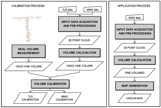
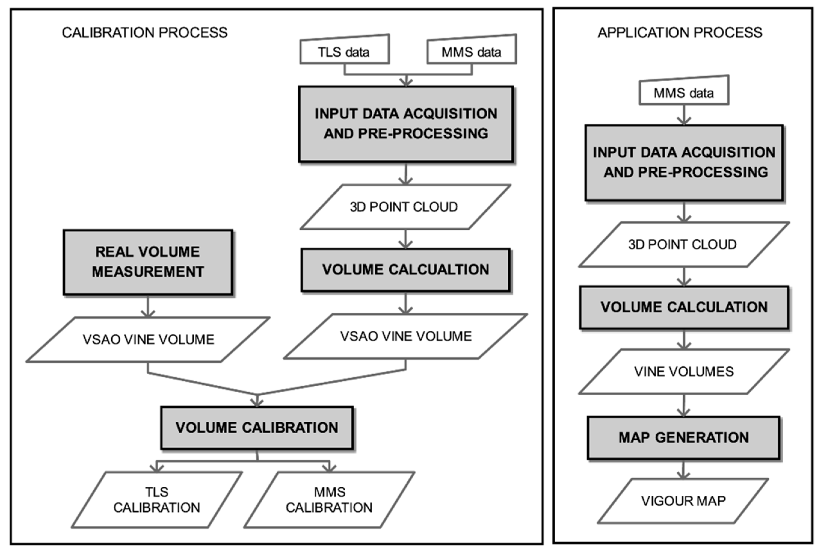
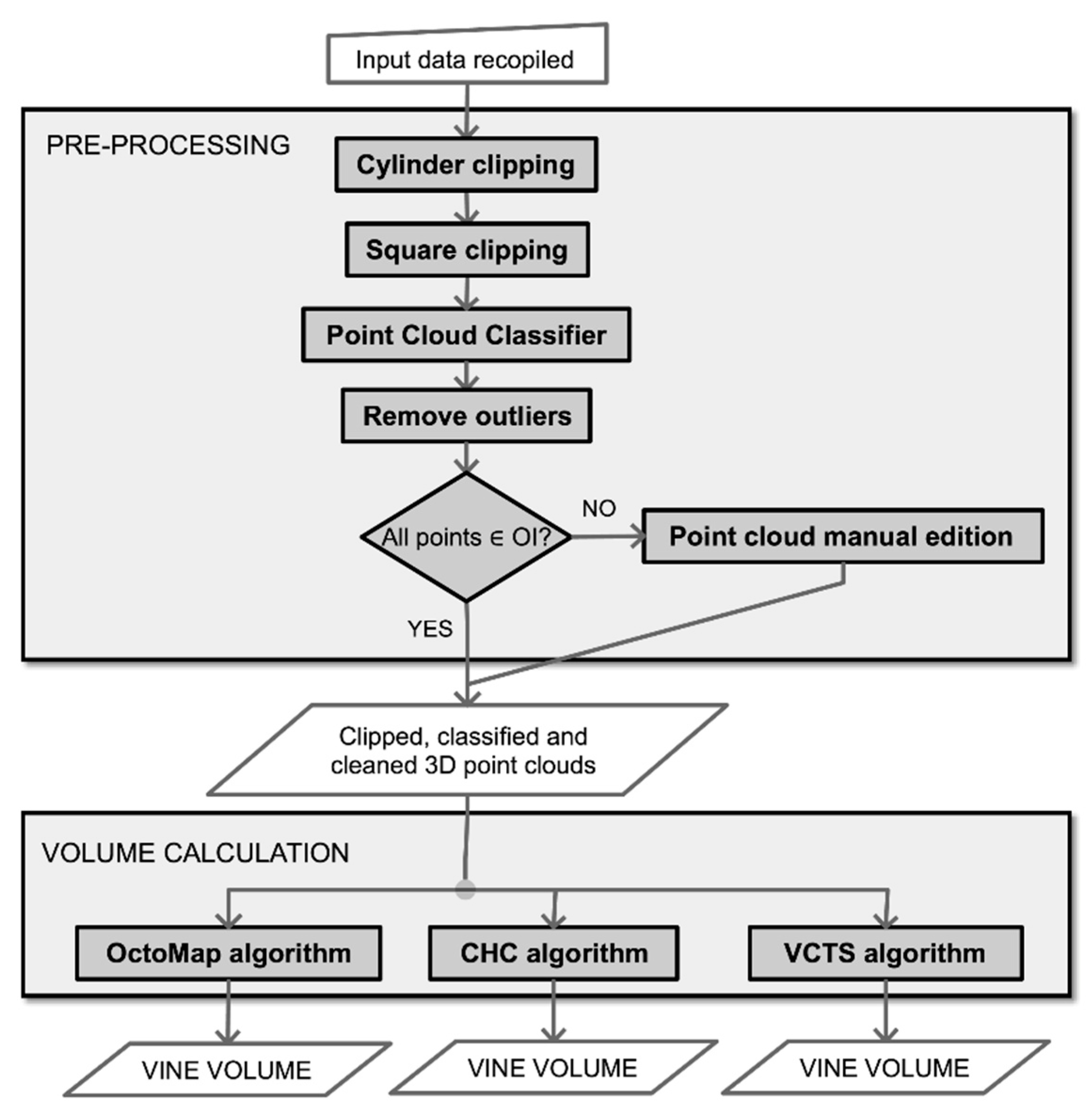
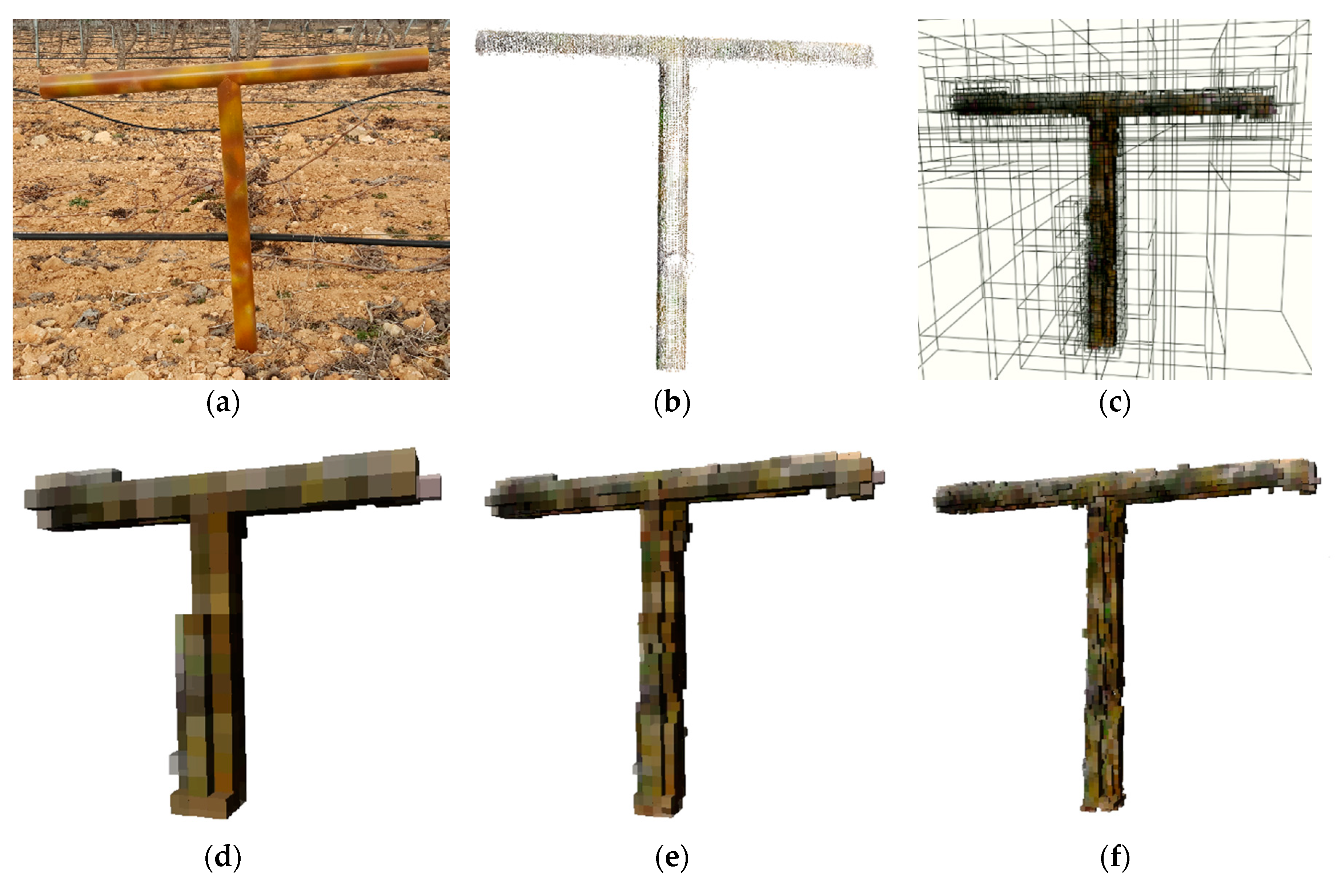
Figure 1 shows the workflow of the proposed methodology. Due to the complexity of the shape of the vines and the non-destructive condition of this study, this study starts with an accurate volume calculation of a vine-shaped artificial object (VSAO) to obtain the real volume data of an object of similar geometry to validate the proposed methodology. The VSAO is composed of two PVC pipes (5 cm in diameter) arranged in a "T" shape, resembling the trunk and the arms of the vineyards driven on a trellis (Figure 2). The choice of the diameter of the pipes used was made according to the average diameter observed in the vines of the vineyard. Likewise, the dimensions and shape of the artificial object were generated by simulating the geometries of the vines in this vineyard. To calculate the volume of the VSAO, the diameter and length of both cylinders were measured.

Field data were acquired and processed for a test area with two laser scanning systems: static terrestrial laser scanner (TLS) and mobile mapping system (MMS). Each piece of equipment produced a colored 3D point cloud with accurate geolocation and high density. These point clouds were the input data used to calculate the volume of the VSAO with specifically developed algorithms. These algorithms, which will be fully described in this manuscript, return the volume of the VSAO from the point clouds obtained with the different systems. After comparing the calculated volume with the actual volume of the VSAO, a volume accuracy can be determined for each system. This process is called the calibration process. Once calibrated, the methodology and the best algorithm will be applied to a real case study on a vineyard located in the southeast of Spain.

2.2. Study Areas for Calibration Process and Application of the Proposed Methodology

A calibration area where the VSAOs were scanned is located in a practice field at the University of Castilla, La Mancha, Albacete (Spain). This vineyard has experimental and teaching purposes, so its state and morphology are highly heterogeneous. However, it covers the typical physical characteristics of trellis systems with a drip irrigation system, where possible occlusions, slope changes, vegetation height, etc., occur. Two identical VSAOs were located in places were vines were missing in positions similar to those of actual vines. Figure 2 shows the location of the two VSAOs in the scanned area. Since the objective was to determine the volume occupied by the vine’s trunk, measurements were obtained without leaves and prunes. This state is the most appropriate for scanning the evidence of crop vigor, because the accumulated vigor appears in the perennial parts of the plant and not in the deciduous parts, such as leaves or prunes.

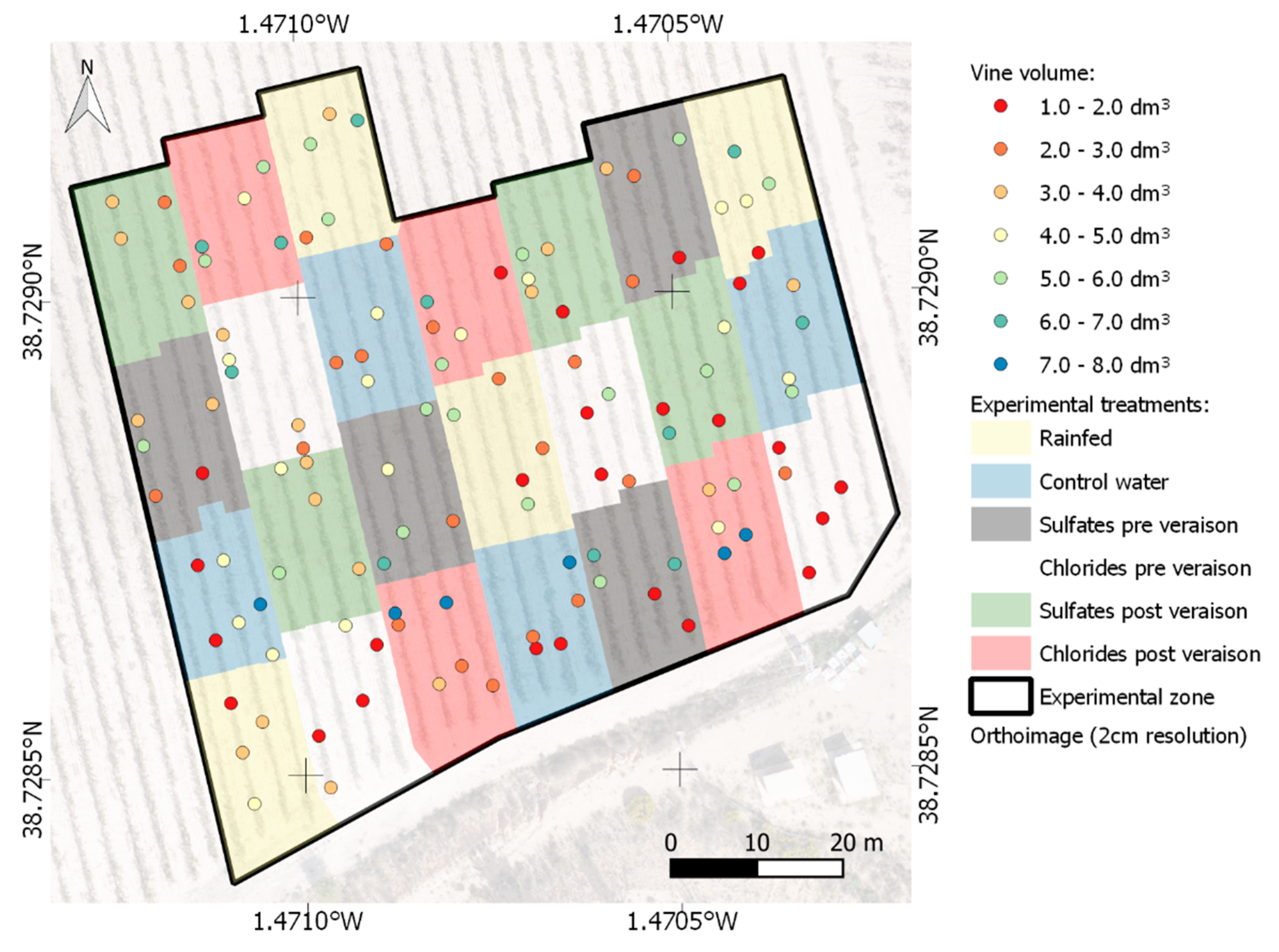
A real application of this methodology was implemented in a vineyard located in the southeast of Spain (38.728928°, −1.470696° EPSG:3857, Figure 3). The study area comprises an area inside of a 0.58 ha vineyard. Trellis driving is separated 3 m between strips and 1.5 m between vines. In this plot, different irrigation treatments have been performed since 2016, as described in Figure 3. These different treatments will, in the future, drive new developments of this canopy. These features make this place an interesting application area due to their high variability. These treatments have been applied only during the last two years, so they have not yet resulted in noticeable differences in the trunk diameter. However, determining plant vigor using the proposed methodology can provide useful information about nutritional and irrigation requirements in the decision making process. Vines with higher vigor would demand more nutrients and water than those with lower vigor. Also of interest is the determination of carbon sequestration by plants, which only accounts for perennial wood and not for shoots or leaves that are removed every year. Thus, with the proposed methodology and data acquisition procedure, vigor maps can be obtained to help farmers better manage their vineyards.

2.3. Equipment

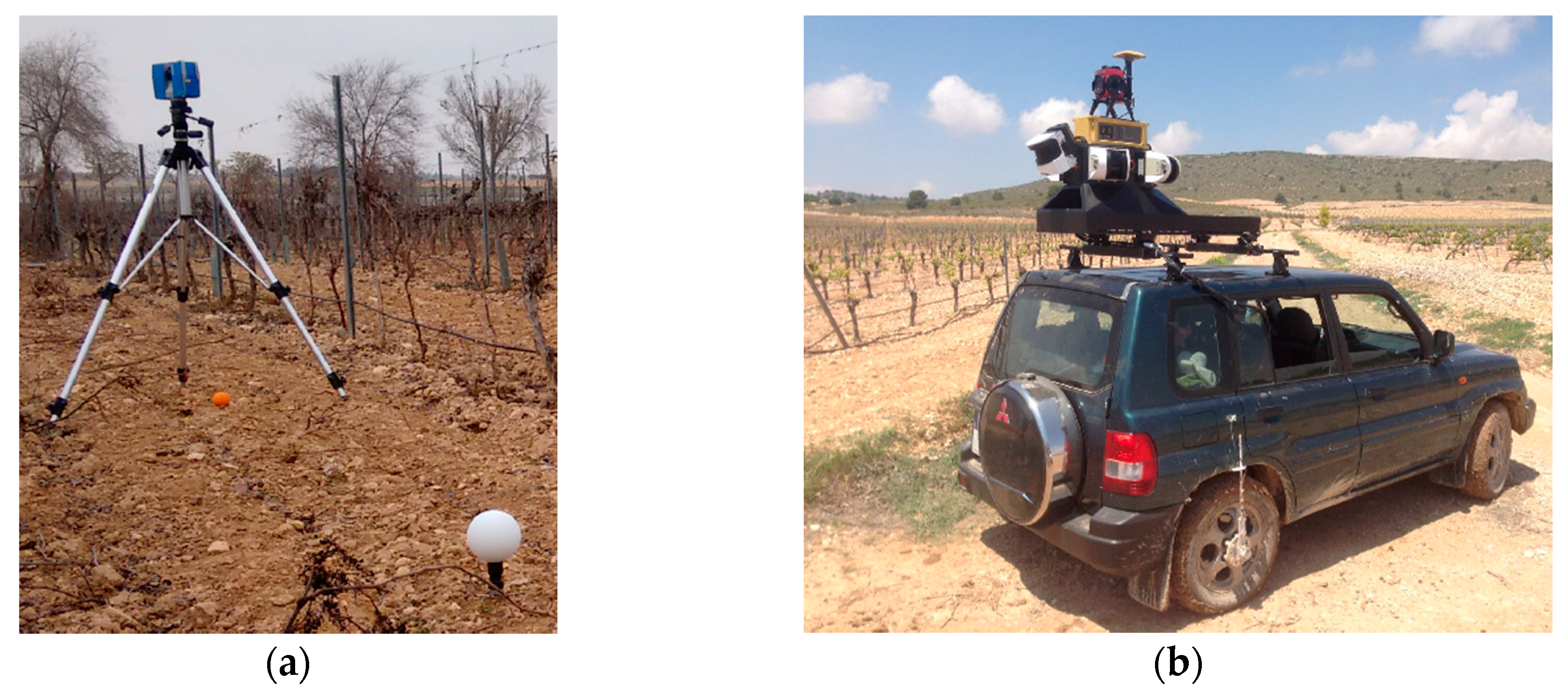
The TLS equipment was a FARO Focus3D X 330 (FARO Technologies, Inc., Lake Mary, Florida) (Figure 4a), which utilizes phase shift technology to read the distance to an object. This reader was mounted on a Manfrotto Super Pro Mk2B tripod and Manfrotto 3D Super Pro head (Manfrotto, Cassola, Italy) (Figure 4a) for each single scan station. This equipment’s field of view is almost complete, with a 360° view on a horizontal plane and 300° on a vertical plane because of its gyratory base and rotation mirror. The scan resolution was configured to 6 mm to 10 m, with a beam divergence of 0.19 mrad (1 cm to 25 m) and a ranging error of ±2 mm (10 to 25 m). It also contains an RGB camera, GPS receiver, electronic compass, clinometer, and altimeter (electronic barometer) to approximately correlate the individual scans in postprocessing. For the accurate joining of different point cloud-calibrated white spheres, an ATS SRS Medium (ATS Advanced Technical Solutions AB, Mölndal, Sweden) was used (Figure 4a). The information captured with this equipment was processed by the software SCENE 6.2 (FARO Technologies Inc., Lake Mary, United States), resulting in a unique georeferenced and colored 3D point cloud.

MMS is a Topcon IP-S2 Compact+ (Topcon Corporation, Tokyo, Japan) (Figure 4b). This is a system that integrates five laser scanners, a 360° spherical digital camera with six optics, an IMU (Inertial Measurement Unit), a dual frequency GNSS receiver, and a wheel encoder. The laser scanners are all SICK LMS511-10100S01 (SICK AG, Waldkirch, Germany), and the spherical camera is a FLIR LadyBug 5+ (FLIR Integrated Imaging Solutions Inc., Richmond, Canada). The system was mounted in a regular 4 × 4 car, with additional batteries and a control system (a high performance rack system, with an i7 processor, 32 GB RAM, and redundant SSD with industrial USB 3.0). The capture software was Topcon Spatial Collect 4.2.0 (Topcon Corporation, Tokyo, Japan). The postprocessing software for the data collected by this equipment was the Topcon Geoclean Workstation 4.1.4.1 (Topcon Corporation, Tokyo, Japan). The resulting product was a georeferenced and colored 3D point cloud. Considering the mobile condition of the equipment and the integration of the sensors, the five possible returns for each laser scanner were filtered to the highest intensity to ensure false observations (noise points).

For the acquisition of geolocation data, we used a GPS-RTK (global positioning system—real time kinematic) with Topcon HiPer V (Topcon Corporation, Tokyo, Japan) receptors and postprocessing software MAGNET Tools 5.1.0 (Topcon Corporation, Tokyo, Japan) in the reference point measurement, using the MMS trajectory solution with centimetric precision.

The main characteristics of both laser scanners are reviewed and compared in

Table 1. The laser scanner’s technical characteristics.

Characteristic	TLS	MMS
Brand and model	FARO Focus3D X 330	Topcon IP-S2 Compact+
Laser principle	Phase shift	Time of Flight
Number of evaluated echoes	1	5
Wavelength	1550 nm	905 nm
Beam divergence	0.19 mrad	11.9 mrad
Maximum scan rate	976,000 points/s	150,000 points/s
Range	0.6 to 330 m	0.7 to 80 m

.

2.4. Data Acquisition

For the calibration process, VSAOs were ubicated on two points where vines were missing, as can be seen in Figure 2. Scanning with TLS and MMS was performed with the spatial configuration shown in Figure 5. Six TLS stations were used, at 1.60 m from terrain, around the two VSAOs. The MMS trajectory was three rows on each side of the VSAO. On the chosen date (February 2019), the crop was pruned, and the sprouting had not yet started to avoid occlusions.

On 11 May 2018, data were acquired for the real case, with the sprouting just having started, so there was no occlusion of leaves. The MMS was driven by all rows of the experimental zone (Figure 3) and the two contiguous rows to each side of the perimeter, to cover all the delimited areas of interest with enough overlap.

2.5. Algorithms for Volume Calculation

Several algorithms that help in the process of volume calculation from point clouds have already been developed [50,51]. However, these are general algorithms that require adaptation and calibration for different object shapes, as well as sparse and noisy point clouds, such as in the case of vine trunk volume calculation. Other algorithms, such as the L₁-medial skeleton [52], can help develop new algorithms for volume calculation, which is one of the main contributions of this paper. The shape of the vine trunks is highly irregular; these trunks are located in an adverse environment for data acquisition, which demands point cloud treatment, algorithm evaluation, calibration, and adaptation. This process should be incorporated in a tool that performs these tasks in an automatic manner. With the methodology and tool developed in this manuscript, these requirements are fulfilled. The proposed methodology includes the development, adaptation, and implementation of a set of algorithms developed in the C++ language and a classification algorithm implemented in MATLAB (Mathworks Inc., Massachusetts, USA); all of these algorithms have been integrated into a unique piece of software.

The imported information includes:

• A text file with the approximate coordinates for each vine base, which can be obtained with a GNSS-RTK or a high resolution orthoimage, among others.
• A text file describing the main parameters of the project: the name, approximate dimension of the searched figure (Figure 6), input and output file paths, formats, coordinate reference systems, etc.
• A point cloud in the LAS file format [53] or compressed LAZ.
• A text file with the position of each single scan performed by TLS.

Three strategies have been implemented and evaluated to calculate the volume occupied by the vine: (1) OctoMap [50], which is an algorithm to generate volumetric 3D environmental models based on voxelization of the occupied space; (2) a convex hull cluster (CHC) [51] that closes the convex envelope of previously clustered sets of points according to geometric and radiometric criteria; and (3) volume calculation from the trunk skeleton (VCTS), which obtains the volume of an object from the distance between each point of the cloud and the internal structure of the object, generated with the L₁-medial skeleton [52] algorithm. These three algorithms will be described below. These are some volume calculation strategies that we have adapted to the characteristics of the point clouds captured by our TLS and MMS. However, none of these strategies are ready to be applied to the specific case of calculating the volume of vine trunks. In this paper, we describe the new developments and adaptations required for the case study of vine volume calculation. This is especially crucial in the case of MMS, where point cloud data are sparse and noisy, but whose applicability is higher due to the wider areas covered. Automated point cloud classification based on RGB values, point selection based on trunk shape, and the development, adaptation, and calibration of algorithms for volume calculation are the main contributions of this work.

Before applying any of these three algorithms, the acquired point cloud should be preprocessed to produce a point cloud with a high quality and three-dimensional definition of the scanned object. If automated clipping, classification, and debugging processes are not enough to define the vine shapes, possible manual editing of the resulting point cloud can be performed. The latter is a step that should be avoided to ensure a highly automatic process.

It should also be noted that the tools for each algorithm (i.e., 3D viewers) have also been incorporated in the implementation of the algorithms used in this work, since most of the modelling libraries from the point clouds include them for their determination and use in different workflows.

The processing steps are summarized in Figure 7. The algorithm implements six different and independent processes that require parameter definitions that are adequate for each datum and can be applied to each vine separately. Intensive work has been performed to determine the parameters that best apply to this case study; these parameters will be shown in results section.

2.5.1. Point Cloud Preprocessing

The raw data collected by TLS and MMS are processed with the software supplied with the equipment—FARO SCENE for TLS and the Topcon Geoclean Workstation for MMS—integrating the information from the different sensors that each system incorporates (Section 2.3). As a result, these software packages return two georeferenced and colored 3D point clouds. However, before applying the algorithms to volume calculation, it is necessary to preprocess the georeferenced and colored point cloud to (1) obtain the point cloud relative to each individual vine; (2) eliminate any point cloud belonging to leaves; and (3) remove any outliers that appear because of the adverse environment in which the measurements were obtained. To perform these preprocesses, software was developed that permits the automated application of this preprocess.

(1) Cylinder and square clipping subprocesses

With the cylinder clipping algorithm, the input point clouds are segmented for each vine as a cylinder with two possible criteria from which to choose the radio: the ROI (region of interest) buffer (found at a half distance between the contiguous vines in its strip) or the fixed distance between vines in the same row. The cylinder centers are determined by the coordinates of the vine base collected by centimetric GPS-RTK measurement.

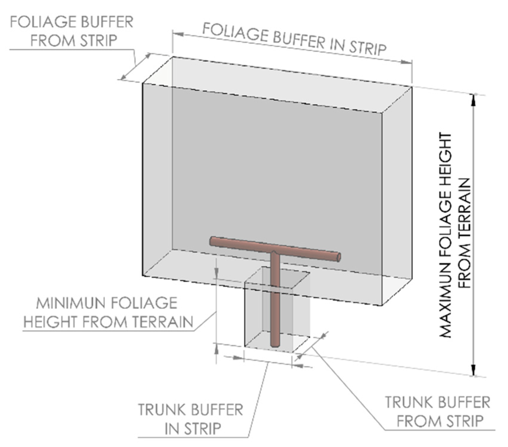
The square clipping step algorithm permits one to approximate cropping to a composed figure of two superposed straight parallelepipeds, one for trunk definition and one for arm definition (Figure 6), depending on the type of pruning performed. In the case study, the scanned vines were pruned with Guyot, so only the trunk was characterized. This process helps to improve the point cloud depuration and removing noise and other elements.

A review of the editable parameters of these two steps is listed in

Table 2. List of the editable parameters of the cylinder and square clipping processes.

Name	Description	Possible Values
ROI 1 buffer	Method to segment first cylinder	fix@distance, computed@halfMeanDistance
Trunk buffer from strip	Length in meters. See Figure 6	0.050 to 0.500
Trunk buffer in strip	Length in meters. See Figure 6	0.050 to 0.500
Minimum foliage height from terrain	Length in meters. See Figure 6	0.100 to 1.000
Maximum foliage height from terrain	Length in meters. See Figure 6	0.400 to 2.000
Foliage buffer from strip	Length in meters. See Figure 6	0.100 to 1.000
Foliage buffer in strip	Length in meters. See Figure 6	ROI buffer, distance (0.500 to 2.000)
Sensor type	Sensor type choice	TLS 2, MMS 3

¹ Region of interest. ² Terrestrial laser scanner. ³ Mobile mapping system.

.

(2) Point cloud classifier subprocess

This process consists of classification according to standardized classes [53]. This allows one to segment the points that define the woody part of the plant in case the canopy is developed. The implemented algorithm is a semi-automatic segmentation of points using only their color. This approach is an application of computational vision techniques based on an artificial neural network (ANN) capable of clustering points with similar radiometric responses. This process has two subprocesses that are clearly differentiated: training a neural network and applying it.

This algorithm is a further development of the leaf area index calculation software (LAIC) [54], which is applied to point clouds. For training, only one vine has to be used. In the input point cloud loading, the RGB color space is transformed into a CIE-Lab color space (Commission Internationale de l’Eclairage (Lab)), where L is lightness, a is the green to red scale, and b is the blue to yellow scale. In this way, we transform the color space of the three components (R, G, and B) to two components (a and b). Then, a cluster segmentation (k-means) is performed on a determined number of clusters (2 to 10), considering this bi-dimensional variable (coordinates a and b). The user then identifies, in a supervised process, which cluster of points represents the woody vine part. With this selected cluster, an ANN is trained. A minimum percentage of successfully classified points with the ANN-calibrated model in the supervised process should be reached (usually 95%). Afterward, the trained ANN is applied to all vines, assigning a class to the points that represent the woody parts of each vine.

The processing parameters for this tool are listed in

Table 3. List of the editable parameters of the point cloud classifier.

Name	Description	Possible Values
Calibrate or apply	Calibrate (1) or apply calibration (0)	1 or 0
Class for trunk	Code classifier as trunk [53]	13 to 31
Hidden nodes	Number of hidden nodes	2 to 15
Input nodes	Number of input nodes	3 to 3
Iterations	Number of iterations	10 to 2000
Minimum calibration accuracy	Minimum percentage of successfully classified points with the ANN 1 calibrated model in the supervised process, %	50 to 100
Output nodes	Number of output nodes	1 to 1

¹ Artificial neural network.

.

(3) Remove outliers subprocess

It is possible that previous processes were not able to accurately segment the vine and required an automatic outlier detection process. This process is parameterized according to the density and disposition of the points expected in the segmented figure. This program implements two different algorithms that are executed consecutively. Both are classes from the Point Cloud Library (PCL) [55], and both are filters of outlier points. The first is the statistical outlier removal [56] algorithm, which detect outliers based on a threshold calculated as the standard deviation of the distance for each point to a certain number of neighboring points. The second algorithm is the radius outlier removal [57]. This filter considers a point as an outlier if the point does not have a given number of neighbors within a specific radius from their location. Detected outliers are classified as a noise point class (Class 7 [53]) in both processes. A list of processing parameters is given in

Table 4. List of editable parameters for the remove outliers process.

Name	Description	Possible Values
Class to use	LiDAR class [53] to use	−1 to 31 1
Statistical sample neighbors for SOR 2 algorithm	Number of sample neighbors to compute mean distance	10 to 1000
Statistical std threshold for SOR algorithm	Threshold of standard deviation of computed mean distance	0.1000 to 10.0000
Radius minimum neighbors for ROR 3 algorithm	Number of minimum neighbors	1 to 1000
Radius search for ROR algorithm	Radius search (meters)	0.0010 to 1.0000

¹ −1 for all classes. ² Statistical outlier removal. ³ Radius outlier removal.

.

2.5.2. Volume Calculation with the OctoMap Algorithm

OctoMap is an algorithm, programmed as an open-source C++ library, to generate volumetric 3D environment models [50]. 3D maps are created by taking the 3D range measurements afflicted with underlying uncertainty. Multiple uncertain measurements are fused into a robust estimate of the true state of the environment as a probabilistic occupancy estimation. The OctoMap mapping framework is based on octrees. Octrees are hierarchical data structures for spatial subdivisions in 3D [58,59]. Space is segmented in cubic volumes (usually called voxels), which represent each node of the octree. Cubic volumes are recursively subdivided into eight subvolumes until the given minimum voxel size is reached (Figure 2 in [50] or Figure 8c). The resolution of the octree is determined by this minimum voxel size (Figure 8). The tree can be cut at any level to obtain a coarser subdivision if the inner nodes are maintained accordingly [50].

Voxels are treated as Boolean data, where initialized voxels are measured as an occupied space (1), and null (0) voxels are free or unknown spaces. It should be noted that we only measured the face of the object shown from the position of the equipment, with existing occlusions. Therefore, each measurement establishes free voxels between the observer and the detected surface (occupied voxel), and all those behind are defined as unknown voxels.

OctoMap creates maps with low memory consumption and fast access time. This contribution offers an efficient way of scanning and the possibility of achieving multiple measurements that can be fused in an accurate 3D scanned environment. In contrast to other expeditious approaches focused on the 3D segmentation of single measurements, OctoMap is able to integrate several measurements into a model of the environment.

Taking advantage of the flexibility of writing data, this framework ensures the updatability of the mapped area, as well as its resolution, and copes with the sensor noise. The state of a voxel (occupied, free, or unknown) can be redefined if the number of observations with different states is higher than the times it was previously observed with its initial state.

Furthermore, the appropriate formulas in the algorithm control the possibility of a voxel to be changed based on its neighbors and the number of times that it has been modified. Thus, the quantity of the data is reduced to the number of voxels that must be maintained. This clamping method is lossless because its thresholds avoid the losses of full probabilities.

The subprocess called OctoMap is an adaptation of the OctoMap algorithm [50] for the purpose of estimating the volume of vines. The editable parameters for the processing point clouds with our adapted algorithm are listed in

Table 5. List of the editable parameters of OctoMap.

Name	Description	Possible Values
Class to use	LiDAR class [53] to use	−1 to 31 1
Compute free voxels	Compute free voxels	True, False
Voxel resolution	Voxel linear resolution in meters	0.0010 to 1.0000

¹ −1 for all classes.

.

2.5.3. Volume Calculation with the CHC Algorithm

The volume calculation algorithm called convex hull cluster (CHC) is the result of the integration of an algorithm from PCL (Point Cloud Library) [52] implemented into our software. It uses the method of voxel cloud connectivity segmentation (VCCS) [51], which generates volumetric over-segmentations of 3D point cloud data, known as supervoxels. These elements are searched as variant regions of k-means clusters through the point cloud (considered a voxel octree structure). They are evenly distributed across 3D space and are spatially connected to each other (Figure 9). Thus, each supervoxel maintains 26 adjacency relations (6 faces, 12 edges, and 8 vertices) in voxelated 3D space with its adjacent neighbors.

The process starts from a set of seed points distributed evenly in space on a 3D grid with an established resolution (R_seed) where the point cloud is located. The voxel resolution (R_voxel) is the established size of the voxel’s edge. The seed voxels begin to grow into supervoxels until they reach the minimum distance from the occupied voxels. If there are no occupied voxels near any point of the cloud among the grown supervoxels, and there are no connected voxels among their neighbors, the isolated seed voxel is deleted.

The seed points are expanded by a distance measure calculated in a feature space consisting of spatial extent (normalized by the seeding resolution), color (the Euclidean distance in normalized RGB space), and normals (the angle between surface normal vectors).

The supervoxels’ growth is an iterative process that uses local k-means clustering.

In this process, confirmed voxels are ignored. In this way, processing is sped up, and the amount of information that needs to be taken into account is reduced. The iterations end when all supervoxels have been confirmed or rejected, and, therefore, all points in the cloud belong to a specific cluster. The editable parameters of the supervoxel clustering are listed in

Table 6. List of the editable parameters of the convex hull cluster.

Name	Description	Possible values
Class to use	LiDAR class [53] to use	−1 to 31 1
Color weight	Weight of color variable	0.000 to 1.000
Normal weight	Weight of normal variable	0.000 to 1.000
Spatial weight	Weight of spatial variable	0.000 to 1.000
Seed resolution	Seed linear resolution (meters)	0.0200 to 2.0000
Voxel resolution	Voxel linear resolution (meters)	0.0010 to 1.0000

¹ −1 for all classes.

.

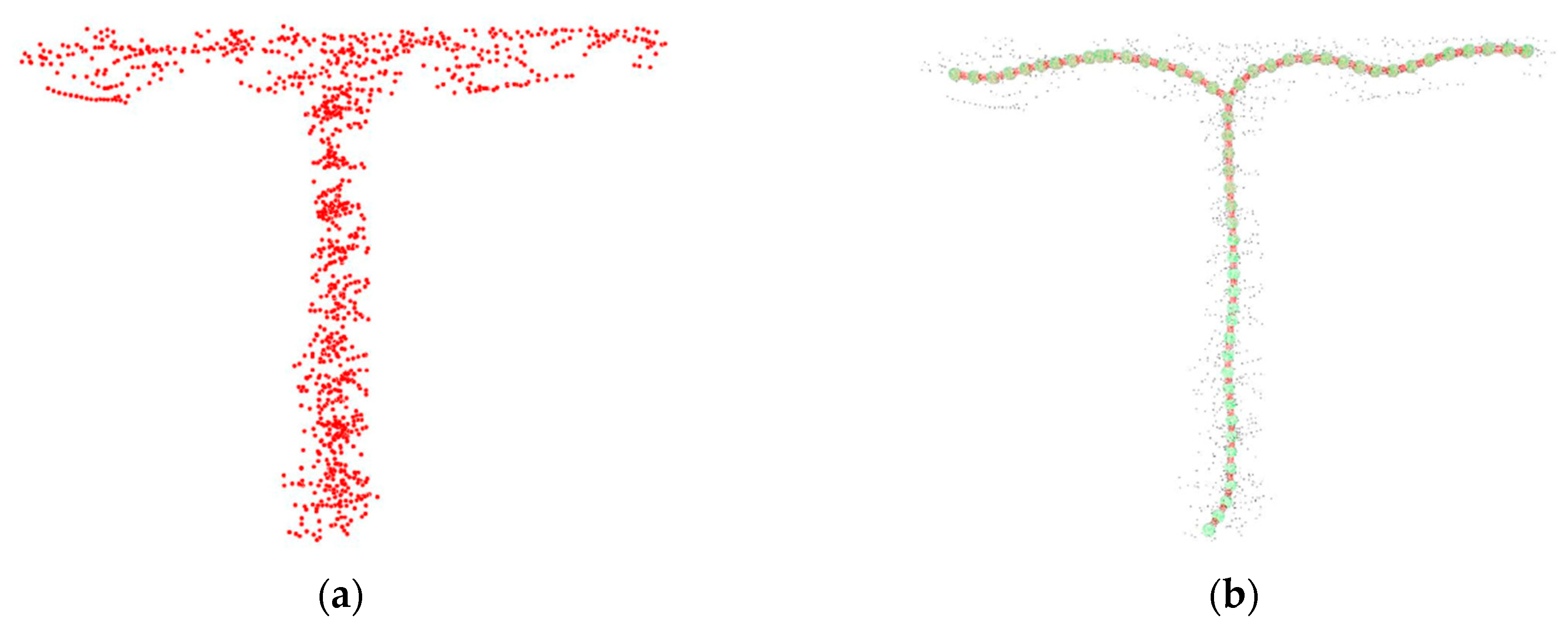
2.5.4. Volume Calculation with the VCTS Algorithm

The L₁-medial skeleton is an algorithm that generates a curved skeletal representation of scanned objects as 3D point clouds. This curved skeleton defines a simplified inner abstraction of the 3D shape of the object, which facilitates analysis of that shape.

This skeleton consists of nodes and segments linked together, as shown in Figure 10. A line string is formed by all segments whose nodes are up to two segments long. The nodes belonging to three (or more) segments define the end of a line string and the beginning of two different line strings.

Although this algorithm is not conditioned by previous assumptions of the geometric shape of the object, we start from the premise that the vine trunk can be modelled as the sum of the volumes enclosed by the cylinders defined by each segment of the skeleton or by the cylinders defined by each line string. Knowing the skeleton and its segments, all the points of the cloud are clustered according to the segment to which they belong. This clustering is based on the proximity of the point to the segment as the minimum (orthogonal) distance between them.

In the first case, the height of each cylinder is taken as the length of each segment. For the estimation of the radius, the parameters of the mean and median centralization of the minimum distances that exist between each point and its segment were used. In the second case, the height of the cylinder is considered to be the sum of the lengths of the segments that comprise it, and the radius as the mean and median of the minimum distances between the points and the segments.

These four volume estimation strategies have been called “VCTS segment mean”, “VCTS segment median”, “VCTS line string mean”, and “VCTS line string median”. These strategies are designed to solve the problem that, for a segment, each point provides a different radius, which can be due to real changes or noise in the point cloud. The success of the algorithm depends on defining a suitable strategy to estimate a single radius value that represents the segment of the object.

To this point, it is necessary to highlight that in the extremes of the vines, the skeleton strategy can fail, because there are few points near the base for the presence of soil, stones, vegetation, and the upper section due to the obfuscation caused by the aperture of the arms. Again, it is necessary to find a strategy to estimate the dimensions of the cylinders at the extremes of the figure. The problems that arise in the clustering of points and the assignation of each segment or string are solved in the following ways:

• The extreme points that are not assigned to any segment or line string (because they are not enclosed between planar sections fixed by nodes and segments) are added to the nearest segment or line string in each case, and extend until they reach the same conditions of belonging as the rest of the points assigned to this segment or line string. This, by default, avoids errors when quantifying the total volume of the vine.
• The assignment to segments or line strings is unique to each point, so all the points are assigned to a single segment or line string, which reduces errors by excess in the zones of insertion between elements (segments or line strings).
• For the mean and median of the L₁-medial skeleton segment, when the segments are given without any assigned point (because the density is not great enough), the radius of the cylinder is considered to be the minimum found in the segments of its line string.
• Because of the low density of the points, their quality and the probability of missing scanned faces, for the VCTS algorithm’s mean and median, if the radius of a cylinder is lower than the mean (or median) radius of the line string to which it belongs in by as many units as the threshold establishes, its radius is considered to be the mean (or median) radius of the line string.

The editable parameters of these algorithms are listed in

Table 7. List of the editable parameters of the VCTS algorithms.

Name	Description	Possible Values
Class to use	LiDAR class [53] to use	−1 to 31 1
Algorithm	Chosen strategy to set radius and height of cylinders	Segment mean, segment median, line string mean, line string median
Minimum outlier threshold	Threshold for elimination of rough errors in meters	0.0010 to 1.0000

¹ −1 for all classes.

.

2.6. Validation Analysis

For the validation of the methods, the absolute and relative errors made in the estimates of the calculation of the volume of both VSAOs carried out with the six proposed strategies were calculated. However, other factors have also been taken into account in order to determine the true possibilities of each sensor and volume calculation algorithm, which will be fully analyzed in the results and discussion. The real value of the volume of each VSAO has been obtained thanks to the simplified form of the pipes that form it. In order to calculate the volume of these artificial objects, the diameter and length of both cylinders that compose them were measured. Afterwards, the equation of the cylinder volume (the circular area of the base multiplied by its height) was applied.

2.7. Generation of Vine Size Maps

Crop vigor maps were elaborated with the GIS (geographical information system) QGIS 3.4.3 Madeira (QGIS Development Team) through volumes calculated by the developed software in relation to the geolocation of each vine. The output data of the implemented algorithms were written to an ESRI Shapefile (Environmental Systems Research Institute, Inc., Redlands, USA) with a geometry type point. Each point feature represented a vine in the vineyard, which included a field with the values of the estimated volumes for each vine. This vector layer was represented with an appropriate graduated color ramp to show, with 7 classes, how vigorous each vine was (its volume). A 2 cm orthoimage of the ground sample distance (GSD) was used as the background layer (the product of the solution of a photogrammetric flight block taken via an airborne RGB camera in an unmanned aerial vehicle (UAV) at a later date). As an aid for the delimitation of the experimental area of this vineyard, the extent of each treatment, and its replications, was also represented. Due to its semi-automatic character, this calculation was applied only to a random selection of 10% of the scanned vines.

3. Results

3.1. 3D Point Cloud Acquisition and Preprocessing

The input data acquisition performed in the test area with the TLS equipment resulted in a colored and georeferenced point cloud. It was performed via six scan stations (Figure 5) with five calibrated spheres as targets for scan joining and georeferencing. The mean target distance error was 9.98 mm and 0.021°, with a deviation of 1.57 mm and 0.009°. The configuration parameters were as follows: a horizontal resolution of 10,240 points, a vertical resolution of 4267 points, a horizontal angular area of 0° to 360°, a vertical angular area of 90° to −60°, and 4× quality.

The GPS positions registered by this equipment have a precision with a 5 m error. Each scan station takes 11.15 minutes.

The same area covered by the MMS collected a colored and georeferenced point cloud. The start and stop angles of its scanners were 65° to 185°, 65° to 185°, −5° to 185°, −5° to 115°, and −5° to 115°. These angles are suitable according to the assembly and position of the scanners in the platform and the occlusions that define the rest of the equipment of the system, including the vehicle itself. The assembly of the scanners can be seen in Figure 4b. The scan frequency was set to 100 Hz, and the pulse repetition frequency (PRF) for the system configuration was 134,000 points per second. The contamination level was set to level 2 for all of them. Level 2, for this equipment, is a high level of contamination that fits the requirement of the agricultural environment in which the data were acquired. The spherical camera captured images in 5 m intervals. The recording of the GPS observations was kept at 10 Hz. The capture lasted 27 minutes and drove 1.7 km due to the maneuvers and the obstacles that the driver of the vehicle had to avoid. The car’s advance speed was set to approximately 1 m/s to increase the cloud point density.

Both clouds were cut with the same defined area of 18.15 m², which included six vines (represented in Figure 5). The TLS cloud had 5,613,180 points, while the one captured with the MMS had 188,984 points.

For data acquisition from the real vineyard, the same capture configuration was used as in the test area. The scanning work was divided into four independent captures of 34, 50, 54, and 35 minutes, covering a total of 27.2 km. It should be noted that despite the size of the scanned area, the vehicle had to find accesses to the strips and have a clear path for kinematic alignment at the beginning of each shot. Thus, the distance travelled far exceeds the actual scanning distance. The environmental acquisition conditions (reflection, dust, etc.) and the characteristics of the equipment’s techniques generated several outliers, which were cleaned with a filter using points based on an intensity value between 225 and 826 and a minimum threshold of four neighbors in a cube with a 0.09 m sized side.

The final point cloud clipped to the experimental zone (0.58 ha; represented in Figure 3) produced 38,833,904 points.

Point cloud preprocessing was done with the parameters reviewed in

Table 8. List of the utilized parameters in preprocessing processes.

Clipping Parameters	TLS2Test Area	MMS3Test Area	MMS Real Case
ROI 1 buffer	computed@halfMeanDistance	computed@halfMeanDistance	computed@halfMeanDistance
Trunk buffer from strip	0.3 m	0.3 m	0.3 m
Trunk buffer in strip	0.3 m	0.3 m	0.3 m
Minimum foliage height from terrain	0.4 m	0.4 m	0.4 m
Maximum foliage height from terrain	1.2 m	1.2 m	1.2 m
Foliage buffer from strip	0.6 m	0.6 m	0.6 m
Foliage buffer in strip	ROI buffer	ROI buffer	ROI buffer
Sensor type	TLS	MMS	MMS
Point Cloud Classifier Parameters	TLS Test Area	MMS Test Area	MMS Real Case
Class for trunk	13	13	13
Hidden nodes	5	5	5
Input nodes	3	3	3
Iterations	60	60	60
Minimum calibration accuracy	95	95	95
Output nodes	1	1	1
Remove Outliers Parameters	TLS Test Area	MMS Test Area	MMS Real Case
Class to use	13	13	13
Statistical sample neighbors for SOR 4 algorithm	50	50	10
Statistical std threshold for SOR algorithm	2	0.5	0.5
Radius minimum neighbors for ROR 5 algorithm	10	2	6
Radius search for ROR algorithm	0.05	0.2	0.09

¹ Region of interest. ² Terrestrial laser scanner. ³ Mobile mapping system. ⁴ Statistical outlier removal. ⁵ Radius outlier removal.

. These parameters were determined by the conditions of the capture. Each situation (sensor, meteorology, crop status, etc.) has specific characteristics to which these parameters have been adapted. The election of dimensional parameters was established considering such aspects as the point density of the clouds, the plantation framework, and the vine size or its prune. For outlier removal, we considered ambient conditions (i.e., dust presence); the skill of the equipment operator and vehicle driver, as well as ground conditions (for constant-speed scanning); and the equipment’s functional requirements and limitations.

Manual editing of the point cloud was done in the segmented vines when the results were anomalous.

3.2. Volume Calculation Results

The processing parameters for volume calculations with OctoMap, CHC, and VCTS are reviewed in

Table 9. List of the utilized parameters in the volume calculation algorithms.

OctoMap Parameters	TLS1Test Area	MMS2Test Area	MMS Real Case
Class to use	13	-	-
Compute free voxels	False	-	-
Voxel resolution	0.01	-	-
CHC 3 Parameters	TLS Test Area	MMS Test Area	MMS Real Case
Class to use	13	-	-
Color weight	0	-	-
Normal weight	1	-	-
Spatial weight	1	-	-
Seed resolution	0.15	-	-
Voxel resolution	0.01	-	-
VCTS 4 Parameters	TLS Test Area	MMS Test Area	MMS Real Case
Class to use	-	13	13
Minimum outlier threshold	-	0.01	0.01

¹ Terrestrial laser scanner. ² Mobile mapping system. ³ Convex hull cluster. ⁴ Volume calculation from the trunk skeleton.

.

These parameters were chosen in an iterative, manual, and supervised process of selection based on the improvement of the results. The visual interpretation of the three-dimensional modelling of each algorithm (whether in the form of voxels, the clustering of points, or simulation of internal structures), and the approximation of the estimated volume to the actual volume of the VSAO, were the criteria for optimizing these values.

The OctoMap algorithm needs to know the precise location of the sensor with respect to each scanned point in order to determine if the resulting voxels represent occupied or undefined space, and, therefore, makes it impossible for us to calculate the volume enclosed by the clouds of points taken with MMS (with this algorithm), as in [60]. In addition, the density of the points attained with MMS does not allow us to calculate the volume of the vines with the CHC algorithm, since the dimensions of some parts (i.e., the trunk’s diameter) exceed the mean density of the cloud; moreover, its precision is low and it lacks the geometric definition of the figure due to occlusions or a lack of perspective when scanning, as in [60]. The results of these volume calculations are shown in

Table 10. Volume calculation results and errors committed.

Scanner	Volume Calculation Algorithm	VSAO 1 A (dm3)	VSAO B (dm3)	Absolute Error (dm3)	Relative Error (%)
TLS 2	OctoMap	2.329	1.666	0.793	28.41
TLS	Convex hull cluster	2.807	2.450	0.179	6.40
MMS 3	VCTS 4 segment median	2.868	2.341	0.264	9.44
MMS	VCTS segment mean	2.863	2.665	0.099	3.55
MMS	VCTS line string median	2.843	2.128	0.358	12.81
MMS	VCTS line string mean	2.916	2.779	0.069	2.46
	Real volume	2.790	2.790

¹ Vine-shaped artificial object. ² Terrestrial laser scanner. ³ Mobile mapping system. ⁴ Volume calculation from the trunk skeleton.

.

The results obtained follow the four strategies proposed for the estimation of the height and radius of the identified cylinders, as shown in Table 10.

Considering these results, the maximum error is reached with the OctoMap algorithm for the cloud scanned with TLS. This is a default error of 28.41%, which may be mainly due to the lack of faces on the scanned object.

The convex hull cluster algorithm improves the volume estimation from this cloud (with a 6.40% error). However, better approximations are given from MMS clouds with strategies based on the calculation of the mean radius per segment (3.55%) and the line string (2.46%).

Figure 8 shows the VSAO (Figure 8a), and the 3D point cloud taken by its TLS (Figure 8b). One can see the lack of scan points where the irrigation pipe is near the VSAO trunk, as well as under its arms. These occluded parts are also visible in the result of the OctoMap algorithm in Figure 8f, where there are no voxels. The same lack of occlusions is visible in the CHC algorithm results (Figure 9b), where it can be observed that the cluster segmented in the arms is thinner than the cluster segmented in the trunk. In both cases, the TLS point cloud underestimates the exterior surface of the VSAO and, consequently, the volume that these two algorithms estimate.

In the same manner, the occlusion of the lower arms is also noticed in the point cloud captured with the MMS equipment (Figure 10a), affecting both the position of the skeleton (not centered) and the determination of the radius of the segmented cylinders (lower than the real value).

3.3. Generation of Vine Size Maps

Based on the results obtained in the validation process, the methodology that achieves the lowest error from the equipment and makes large-scale data collection (MMS) feasible in a real case study was applied. This methodology applies the VCTS line string mean algorithm to 10% of the total scanned strains (120 vines of 1203 vines), which were randomly selected. In the final generated map (Figure 11), values between 1.0 and 8.0 dm³ are observed. This variability may be due to various factors such as new vines planted to replace vines with problems, the lack of consistency in pruning methods, increased occlusions, uneven scanning speed, and other reasons for managing a vineyard or the technical limitations of the scanning method with this equipment in this type of scenario. No differences between the treatments were found (as expected), because these differentiated treatments started only two years ago. We expect to find these differences in the volume of the canopy but not in the trunk volume.

It should be noted that the operational character of the MMS equipment allows a complete mapping of the vineyard with an acceptable density of points, as can be seen in Figure 12.

4. Discussion

It should be noted that the technical limitations of each piece of equipment have guided this work in its two subobjectives: to test the possibility of calculating the volume occupied by the trunks of vines in a vineyard using clouds from points taken with TLS equipment, and to extrapolate the best possibility to a real case study scanned with MMS, where it would be feasible to elaborate a vine size map based on the volume of each vine.

Firstly, the TLS point clouds have digitalized, with high detail and precision, the areas of the vines that were within their reach. Nevertheless, the areas occluded behind the equipment itself or its intermediate elements were not captured, thus making the three-dimensional definition of the scanned object incomplete (in this case, the vines of the vineyard), similar to the problems found in [61]. Secondly, the mobile capture system of the MMS solves this deficiency, as the number of views taken of the object covers most of its faces. This result could be achieved by increasing the number of TLS scan stations, but, considering the large number of faces these objects have, this process would be too costly for the intended purpose. However, the point density and low-quality cause other problems (also treated in [21]). Thus, the approach to treat and evaluate the obtained data should be different. In fact, the different algorithms implemented obtained different results depending on the scanning systems utilized because of the differences in the types of information acquired.

Taking advantage of the TLS (detail and precision) and considering their limitations (occlusions), the two proposed algorithms (OctoMap and CHC) can estimate the volume occupied by the scanned vines with the proposed methodology. OctoMap does not need to know the entire figure if the occlusions are smaller than the calculated voxel size [50], which makes this method appropriate for TLS, where many faces of the object are occluded. Indeed, we identified a defect error in the results due to the occlusion of the lower face of the arms, which could be solved by placing the scan stations at a lower height from the ground. The CHC algorithm is not as strongly affected by this lack of scanned faces since in the case of figures with simple geometries, such as cylinders, the closing of the convex envelopes of the point groupings obtained by this algorithm is accurate and resolves the occlusions suffered by the cloud.

Nevertheless, the capture performance of the TLS makes it unfeasible to survey large extensions of land, such as those covered by agricultural crops. However, the application of the tested algorithms to MMS point clouds is not possible because they have lost the precision and definition conditions required by OctoMap and CHC. In addition, those two algorithms also resulted in lower accuracy in the determination of the VSAO volume for TLS. Thus, it can be concluded that OctoMap and CHC are not the most appropriate algorithms for this case study. We recommend increasing future efforts in developing strategies for the skeleton algorithm.

The proposed change of strategy that focuses on modelling algorithms based on the internal structure of the objects (L₁-medial skeleton [52]), and not on determining the closure of their surfaces (OctoMap [50] and CHC [51]), has made it possible to estimate the volumes of individualized vines scanned with MMS point clouds, as the results show. Even the estimation of volume with this strategy improves, in some cases, the values obtained with TLS clouds (3.55% and 2.46% errors for the VCTS segment mean and line string mean, respectively, compared with a 6.40% error with the CHC algorithm and TLS point clouds). However, in the case of a TLS in which two faces of the trunk are perfectly defined but there are many occlusions because of the lack of perspective, the skeleton algorithm returned many errors that require further development to be robust and usable.

The extrapolation of this methodology to a real case study has identified several alterations that make it difficult to obtain the individualized volumes, which should be overcome in future work. On the one hand, the segmented point clouds of some vines do not define their shape due to the poor quantity and quality of the scanned points. This makes manual additions to the cloud subjective, in order to clean outliers that have not been identified, which is also seen in previous automatic processes, and contributes to the generation of incoherent skeletons. Therefore, the volumes obtained in these cases are inaccurate due to poor quality data acquisition, which can be solved by a better vehicle to transport the MMS, avoiding the generation of dust, decreasing the speed (to increase point density), and maintaining constant speed, among many other factors. On the other hand, strategies based on the VCTS algorithm are semi-supervised and require visual inspection of the generated skeleton before applying the volume calculation. Consequently, this methodology is time-consuming and materially cost-intensive. The increase in the costs that this methodology would require is also affected by the number of vines that require manual editing because of anomalies. Thus, the more variable the scanned noise is, the less the cleaning can be automated, and the more manual editing is needed. More effort towards the complete automation of this process should be developed, because it is the most promising algorithm with this objective.

As probable areas of work based on this experience, improvements will be developed in the automation and handling of algorithms. Further, it will be necessary to improve the conditions during data acquisition, taking into account the generation of dust, the constant speed of the vehicle during data acquisition, and other factors. In addition, since these are parameterized algorithms, their evaluation and optimization for each case study is necessary, so we intend to develop methods that consolidate an appropriate choice based on the improvements that occur in the acquisition of point clouds. Of course, more algorithms that allow the estimation of volumes will be tested, as in [62]. Another challenge to address is the determination of the volume occupied by the canopy (not only the trunk), which will require other algorithms and software development.

Thus, the proposed methodology and developed software are the first step towards promising technology to characterize the geometry of woody crops in order to help decision-making in crop management.

5. Conclusions

In this work, different strategies for calculating vine volumes from point clouds captured with static and mobile terrestrial laser scanners were developed in order to elaborate maps of the vegetative vigor of crops, particularly vine size. The proposed methodology makes use of laser scanning systems in precision agriculture, a promising technology; however, the experience has left several improvements to be solved to improve the obtained results, such as (1) improving the data acquisition; (2) increasing the automation of the result generation to avoid current manual data treatments; and (3) refining the algorithms to better determine the volume.

The results have revealed that the calculation of volumes from different scanning systems requires different algorithms because of the variability in the density of point cloud, noise, and occlusions. TLS point clouds are more accurate using the CHC [51] algorithm (with a 6.40% relative error), while the most complete and accurate results are obtained from MMS point clouds using the VCTS with the L₁-medial skeleton [52] line string mean algorithm (2.46% relative error). The VCTS could not be applied to TLS because of the occlusions that appear with this system, but considering the results using MMS, it is an interesting algorithm to apply to these systems after its adaptation.

The potential of laser scanning equipment has been demonstrated in agronomic challenges, as well as the application of three-dimensional point clouds to the three-dimensional digital characterization of vegetation. However, in this first approach, an intensive manual editing process is required, which should be solved in future developments. Nevertheless, these are the first experiments with this technology, and outstanding results were obtained by this working group, so future prospects are positive.