Detecting Ecological Changes with a Remote Sensing Based Ecological Index (RSEI) Produced Time Series and Change Vector Analysis


Abstract

1. Introduction
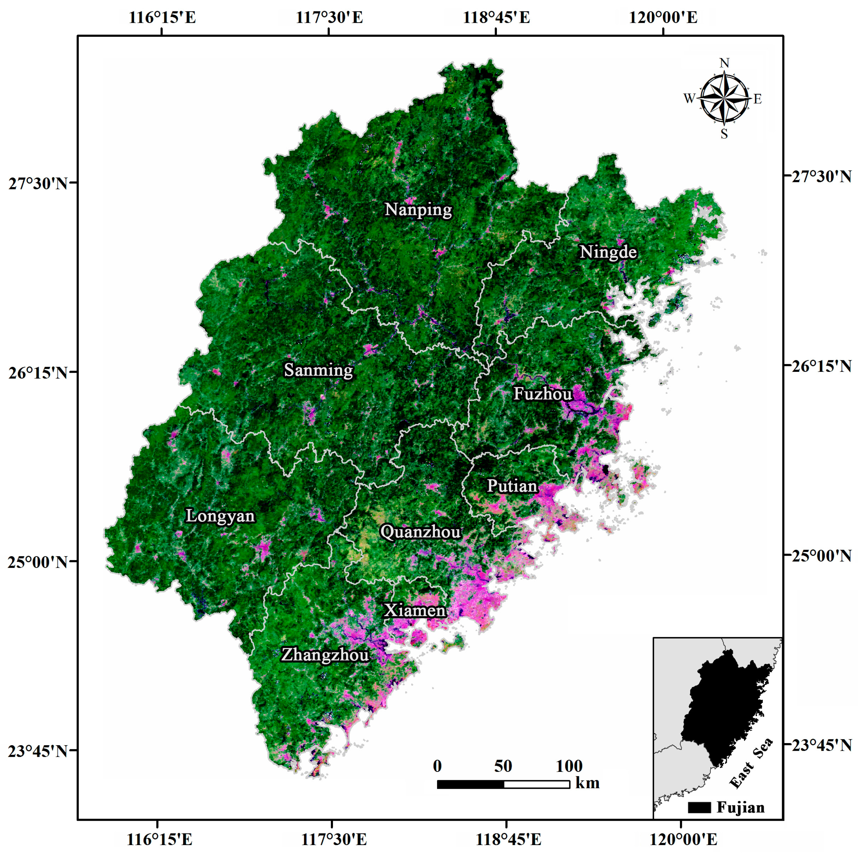
2. Study Area
3. Methods
3.1. Satellite Data
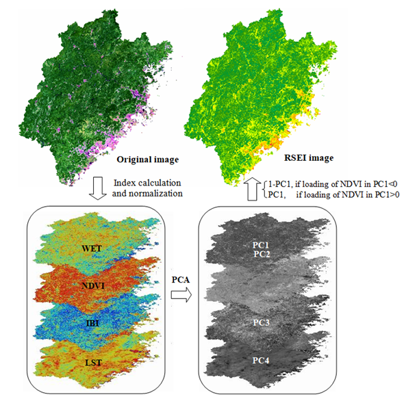
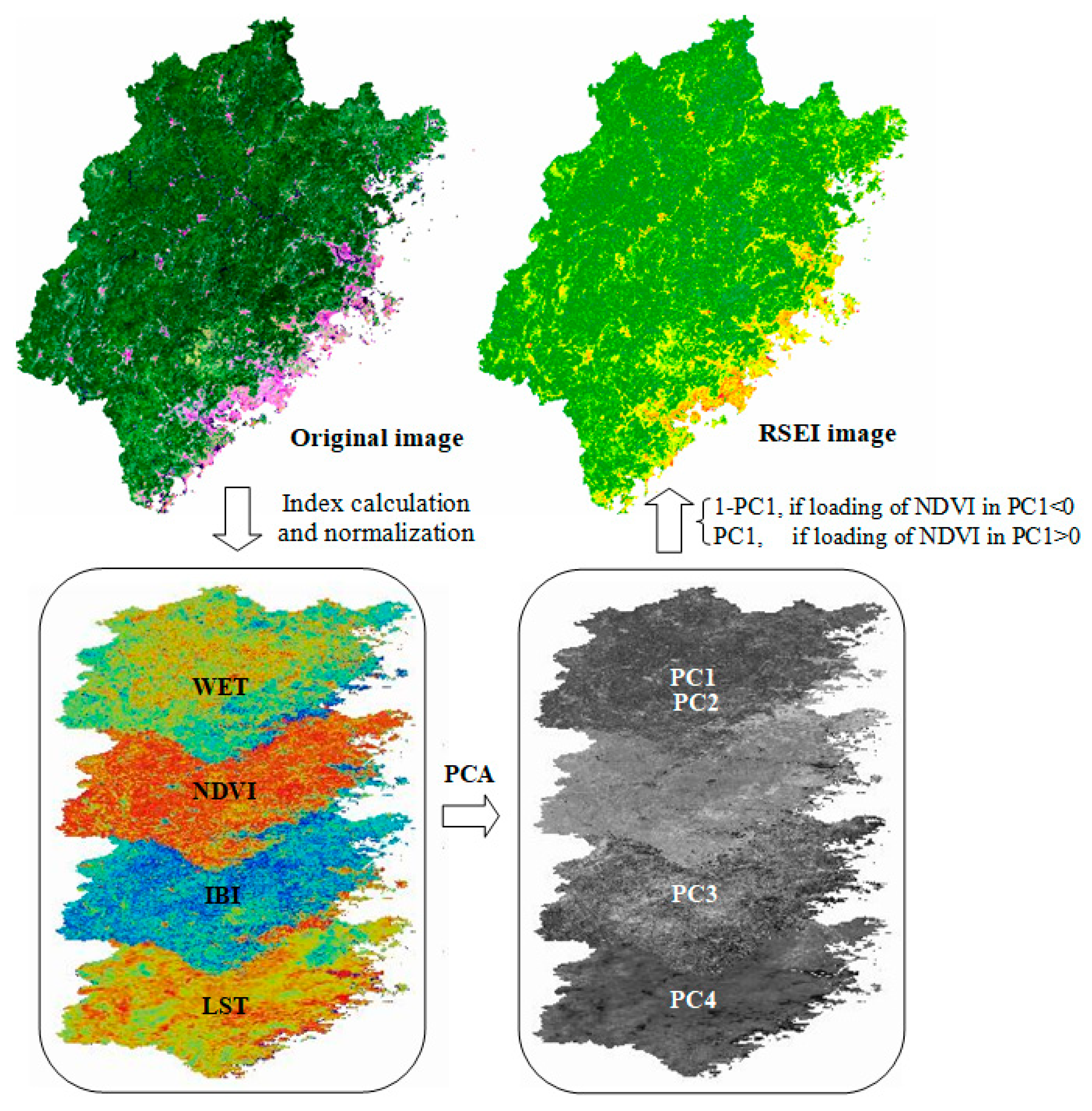
3.2. RSEI Ecological Index
3.2.1. Indicators Used in RSEI
3.2.2. Integration of the Indicators
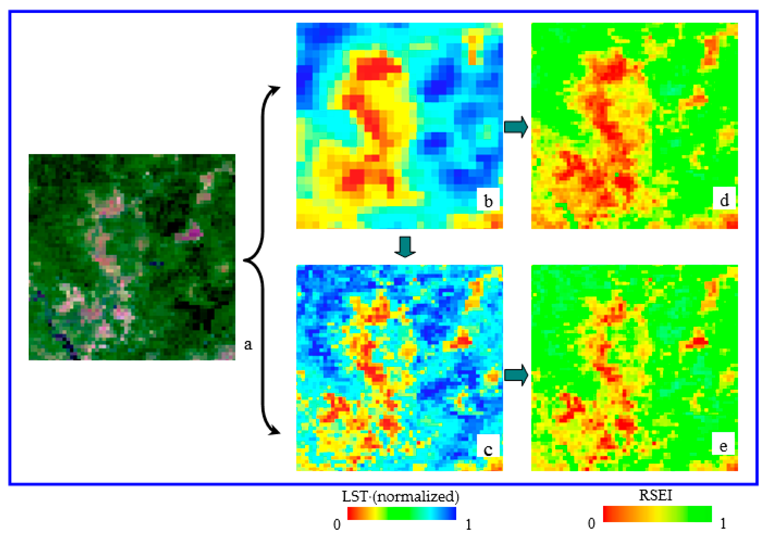
3.2.3. Improvement of RSEI
3.2.4. Detecting Ecological Changes
3.2.5. Statistical Analysis
4. Results
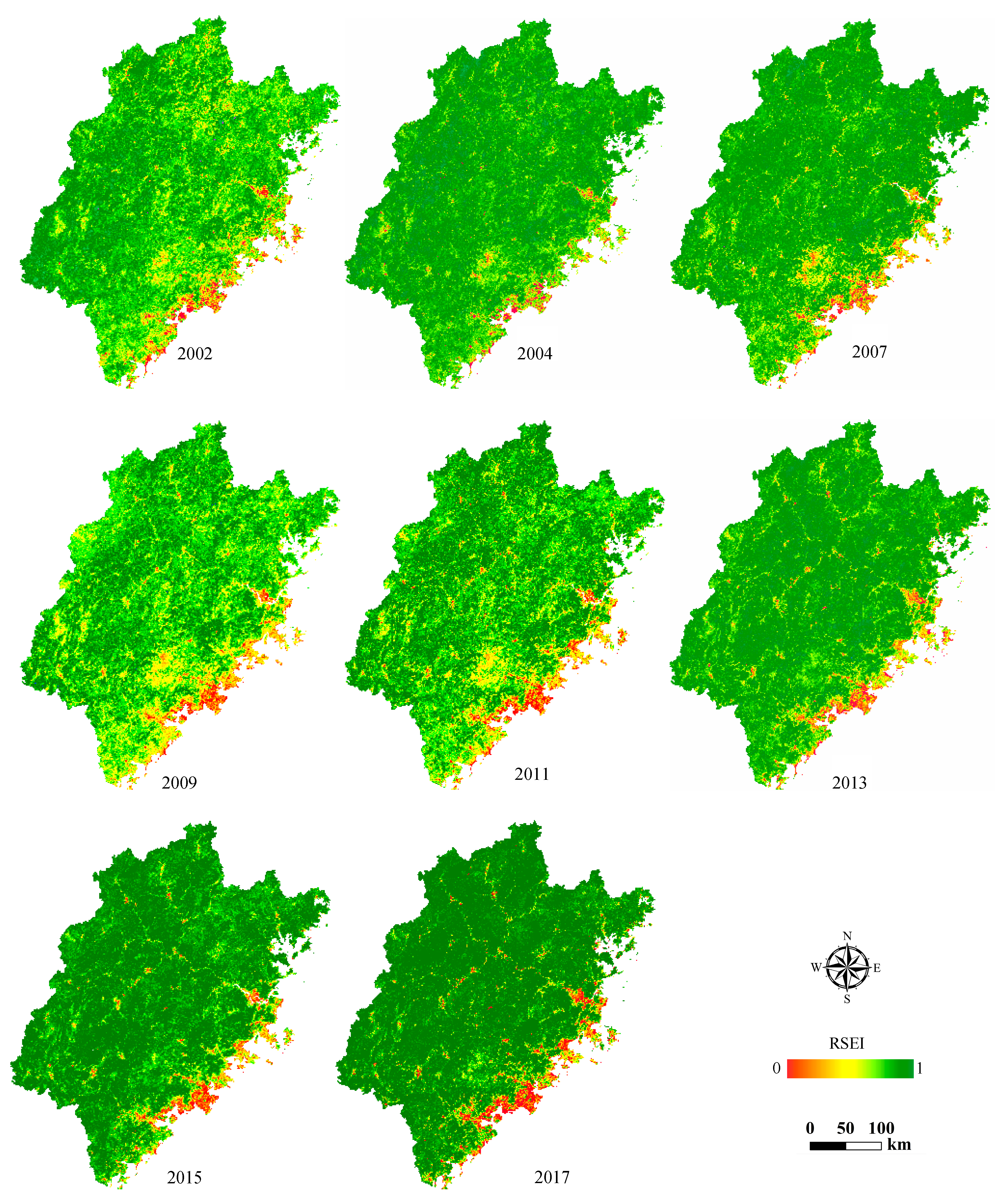
4.1. Ecological Status
4.2. Spatiotemporal Ecological Changes
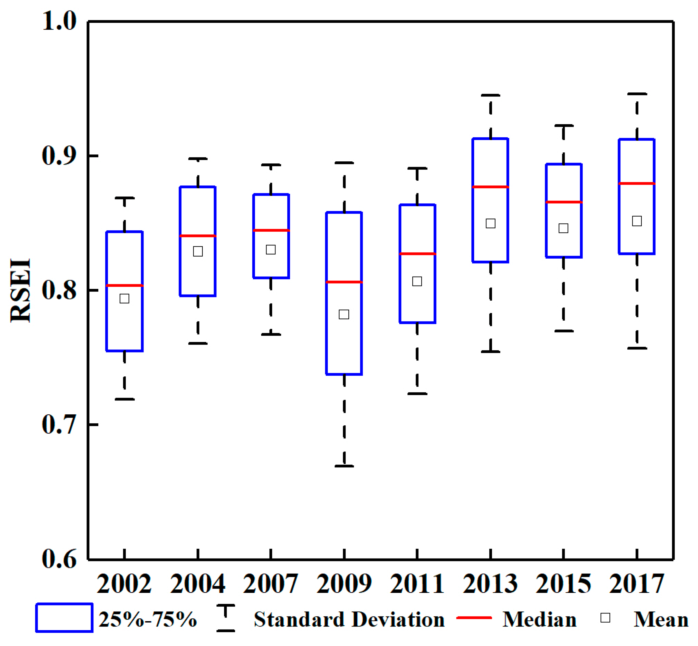
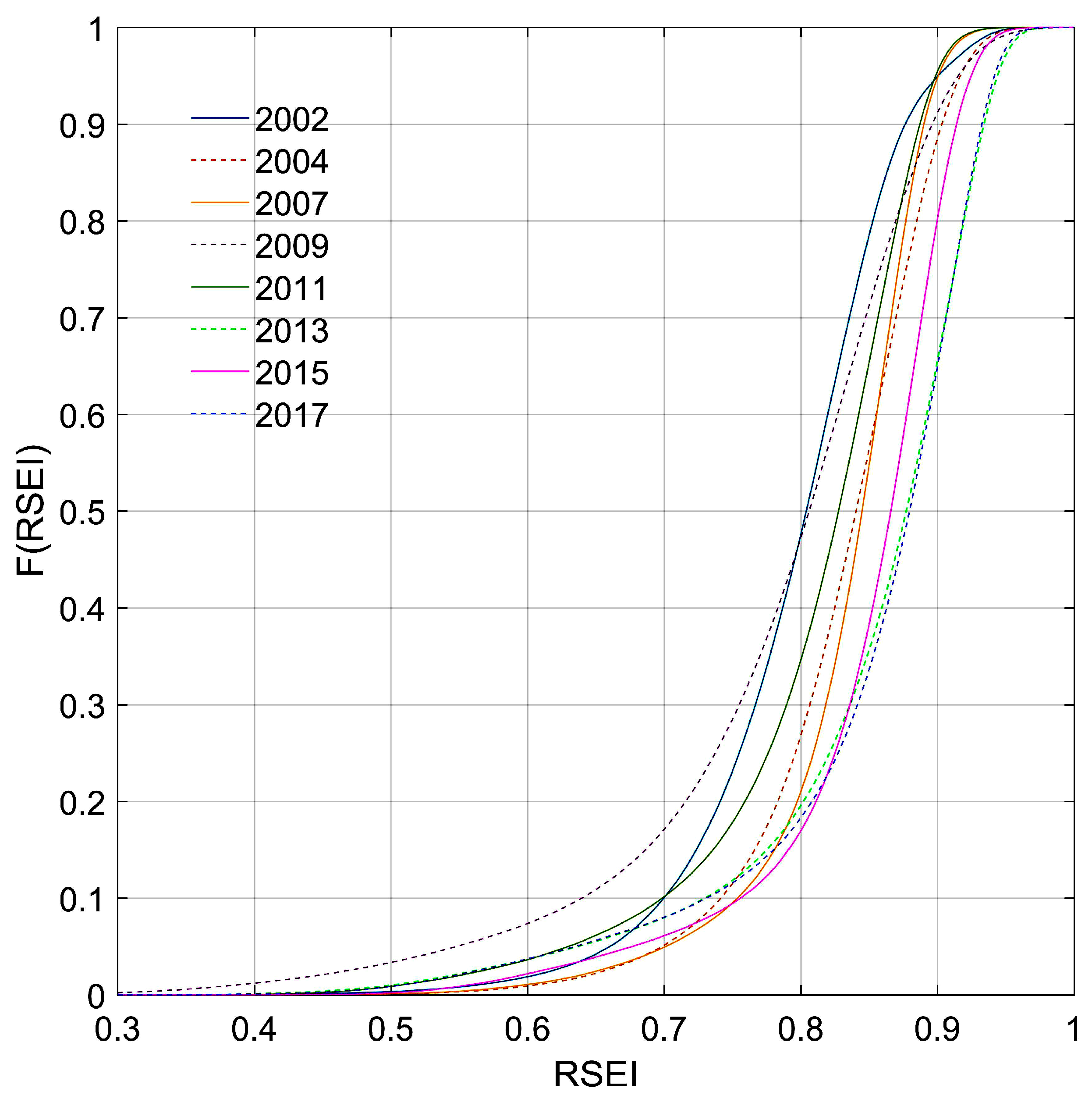
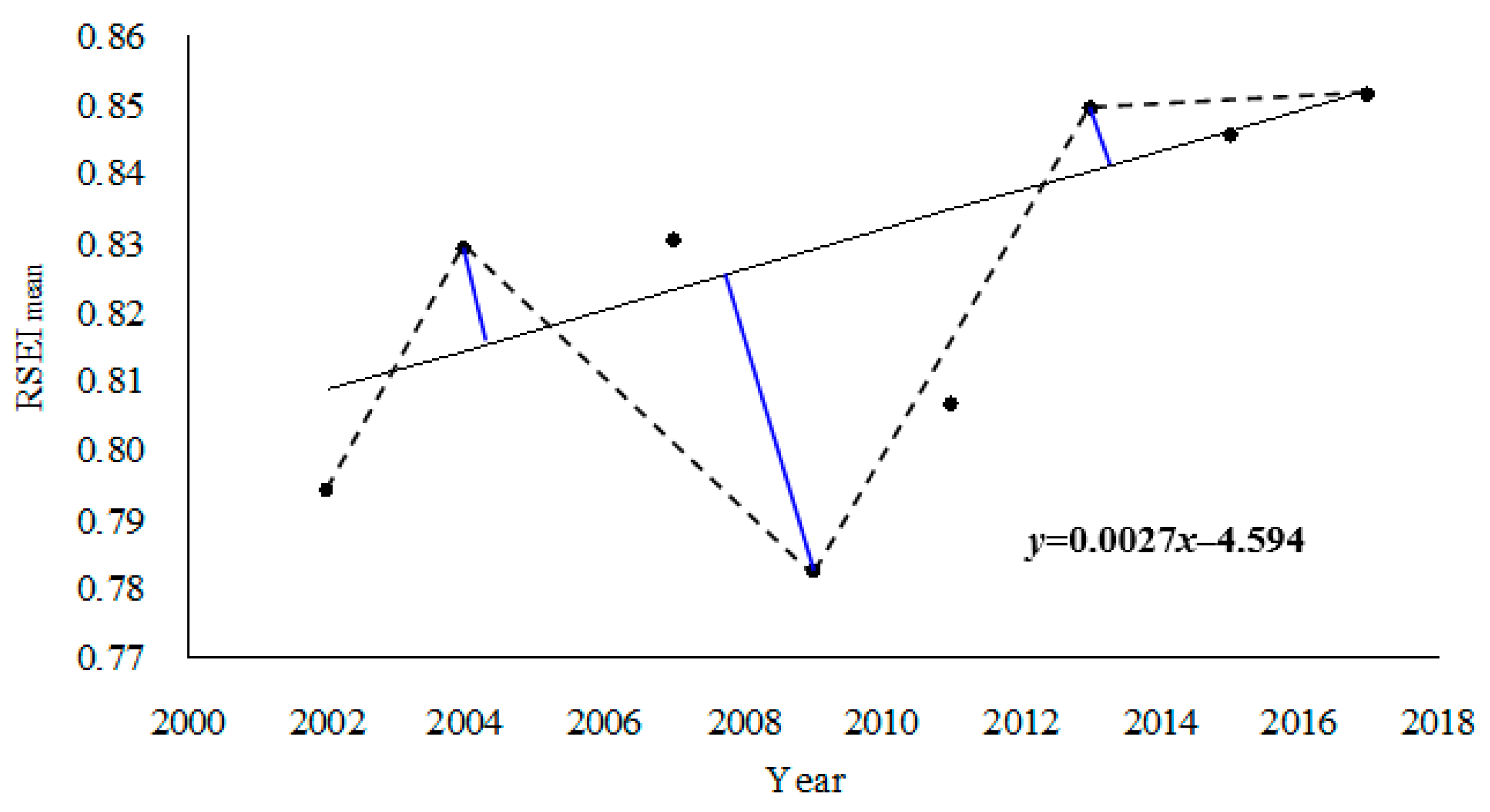
4.2.1. Temporal Change Analysis
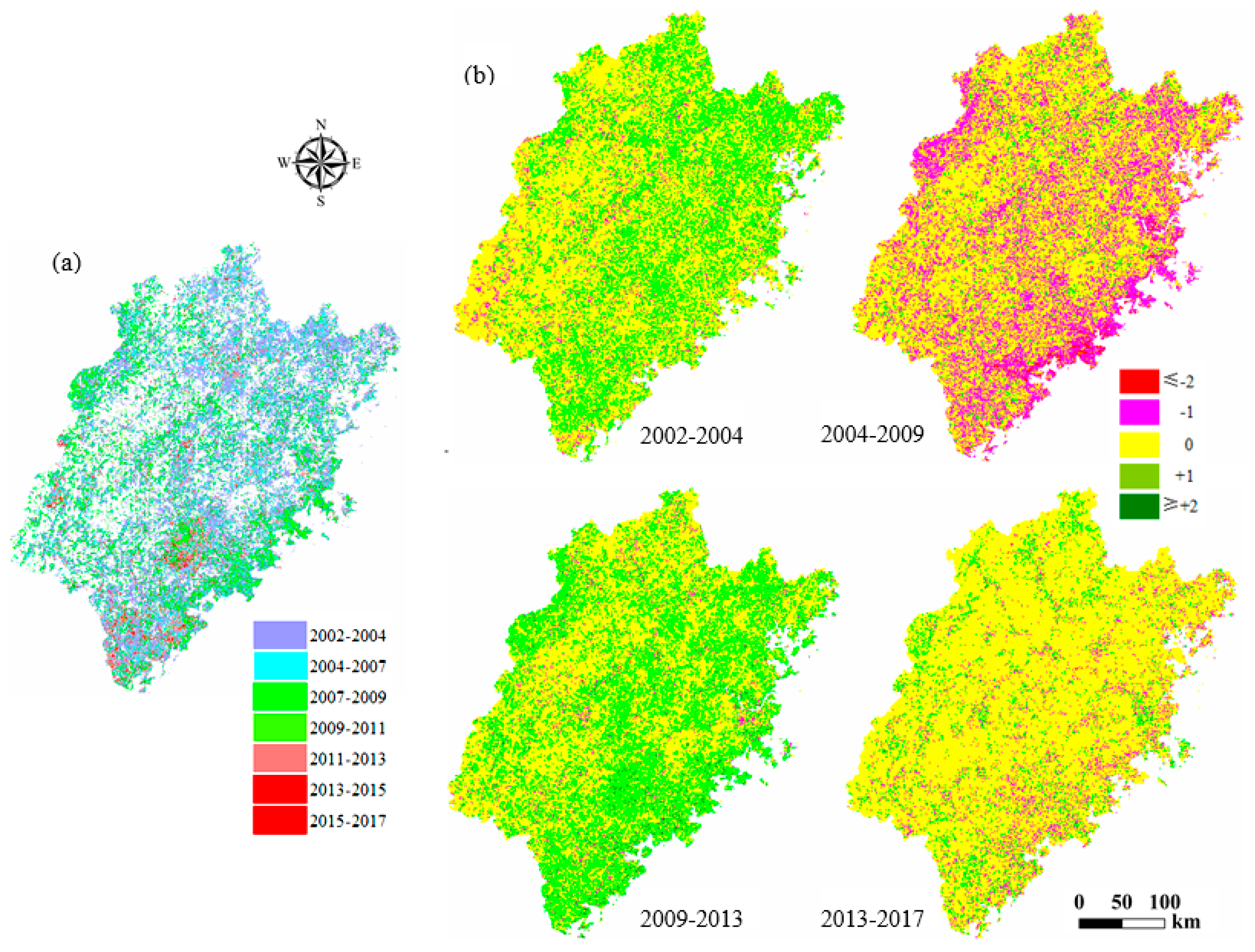
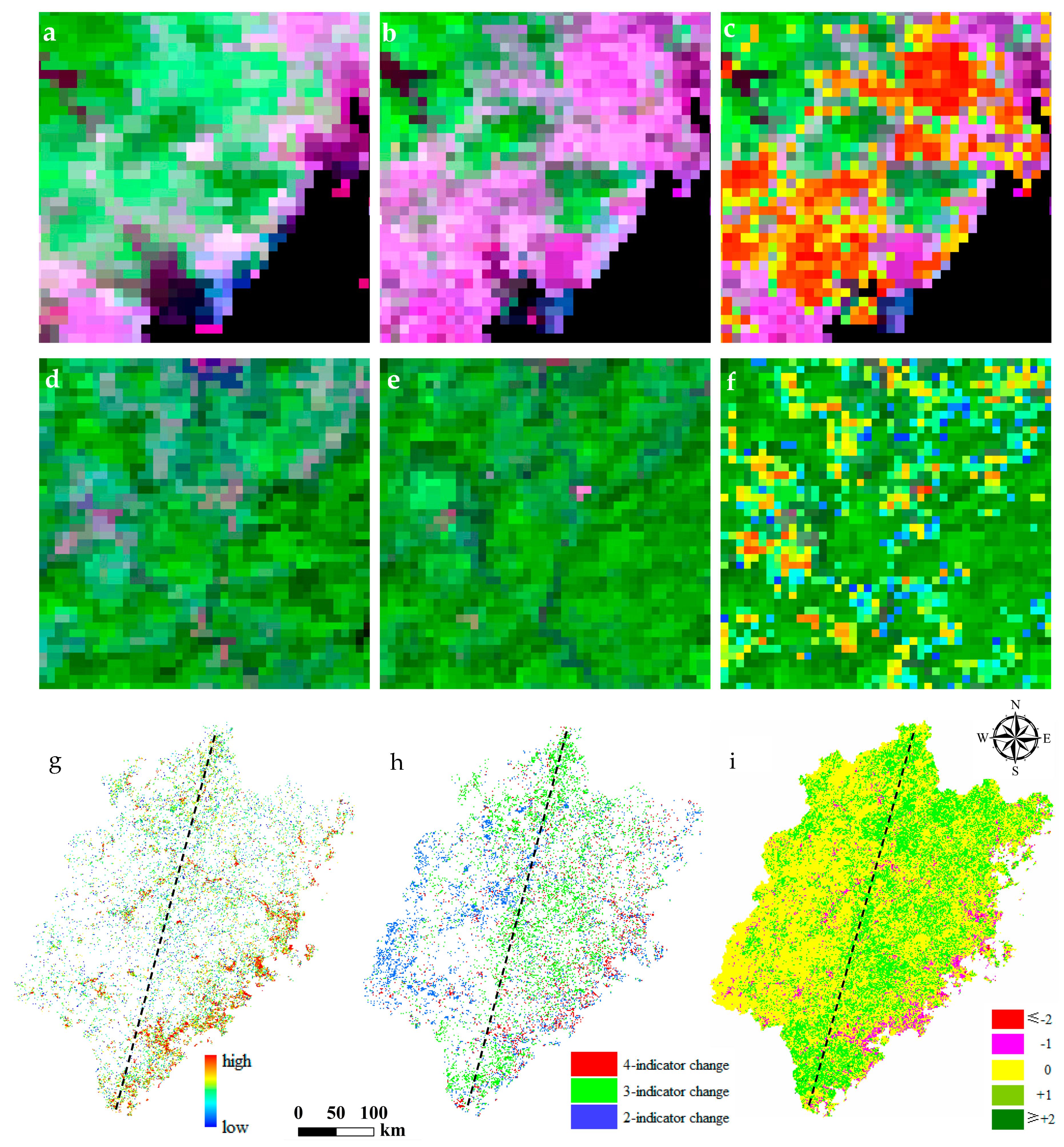
4.2.2. Spatial Change Analysis
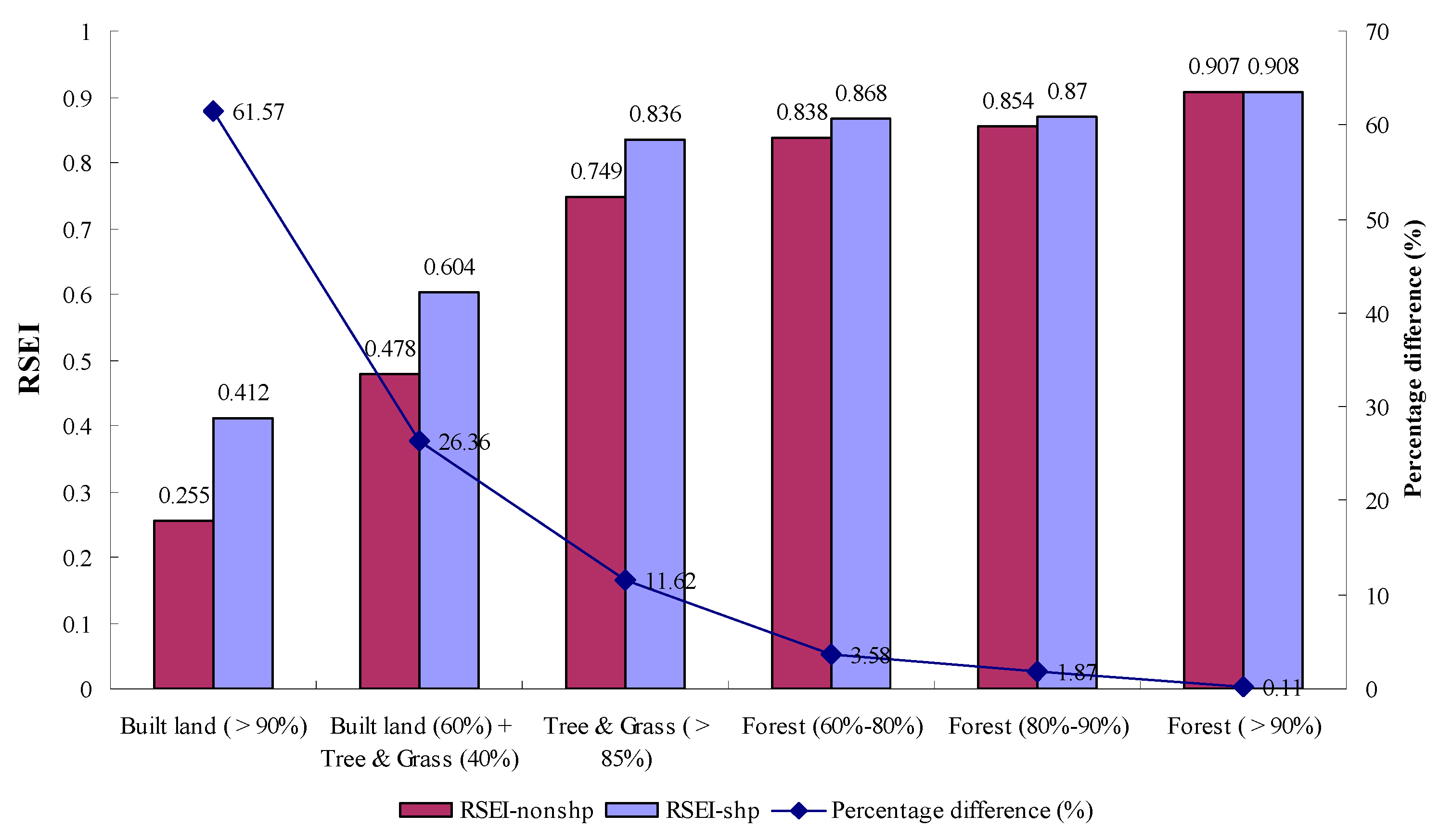
4.3. Comparison of RSEIs Computed with and without Sharpened LST
4.4. Comparison of RESI with Existing Ecological Indices
5. Discussion
6. Conclusions
Supplementary Materials
Author Contributions
Funding
Acknowledgments
Conflicts of Interest
References
- McDonnell, M.J.; MacGregor-Fors, I. The ecological future of cities. Science 2016, 352, 936–938. [Google Scholar] [CrossRef] [PubMed]
- Williams, M.; Longstaff, B.; Buchanan, C.; Llanso, R.; Dennison, W. Development and evaluation of a spatially-explicit index of Chesapeake Bay health. Mar. Pollut. Bull. 2009, 59, 14–25. [Google Scholar] [CrossRef] [PubMed]
- Baldocchi, D. Breathing of the terrestrial biosphere: Lessons learned from a global network of carbon dioxide flux measurement systems. Aust. J. Bot. 2008, 56, 1–26. [Google Scholar] [CrossRef]
- Levin, S.A. The problem of pattern and scale in ecology: The Robert H. MacArthur Award Lecture. Ecology 1992, 73, 1943–1967. [Google Scholar] [CrossRef]
- Qiu, B.W.; Chen, G.; Tang, Z.H.; Lu, D.F.; Wang, Z.Z.; Chen, C. Assessing the Three-North Shelter Forest Program in China by a novel framework for characterizing vegetation changes. ISPRS J. Photogramm. 2017, 133, 75–88. [Google Scholar] [CrossRef]
- Willis, K.S. Remote sensing change detection for ecological monitoring in United States protected areas. Biol. Conserv. 2015, 182, 233–242. [Google Scholar] [CrossRef]
- De Araujo Barbosa, C.C.; Atkinson, P.M.; Dearing, J.A. Remote sensing of ecosystem services: A systematic review. Ecol. Indic. 2015, 52, 430–443. [Google Scholar] [CrossRef]
- Kwok, R. Ecology’s remote-sensing revolution. Nature 2018, 556, 137–138. [Google Scholar] [CrossRef]
- Reza, M.I.H.; Abdullah, S.A. Regional Index of Ecological Integrity: A need for sustainable management of natural resources. Ecol. Indic. 2011, 11, 220–229. [Google Scholar] [CrossRef]
- Ivits, E.; Cherlet, M.; Mehl, W.; Sommer, S. Estimating the ecological status and change of riparian zones in Andalusia assessed by multi-temporal AVHHR datasets. Ecol. Indic. 2009, 9, 422–431. [Google Scholar] [CrossRef]
- Kennedy, R.E.; Andréfouët, S.; Cohen, W.B.; Gómez, C.; Griffiths, P.; Hais, M.; Healey, S.P.; Helmer, E.H.; Hostert, P.; Lyons, M.B.; et al. Bringing an ecological view of change to Landsat-based remote sensing. Front. Ecol. Environ. 2014, 12, 339–346. [Google Scholar] [CrossRef]
- Xu, H.Q.; Wang, M.Y.; Shi, T.T.; Guan, H.D.; Fang, C.Y.; Lin, Z.L. Prediction of ecological effects of potential population and impervious surface increases using a remote sensing based ecological index (RSEI). Ecol. Indic. 2018, 93, 730–740. [Google Scholar] [CrossRef]
- Ouyang, Z.Y.; Wang, Q.; Zheng, H.; Zhang, F.; Hou, P. National ecosystem survey and assessment of China (2000–2010). Bull. Chin. Acad. Sci. 2014, 29, 462–466. [Google Scholar]
- Caccamo, G.; Chisholm, L.A.; Bradstock, R.; Puotinen, M.L. Assessing the sensitivity of MODIS to monitor drought in high biomass ecosystems. Remote Sens. Environ. 2011, 115, 2626–2639. [Google Scholar] [CrossRef]
- Rouse, J.W.; Haas, R.H.; Schell, J.A.; Deering, D.W. Monitoring vegetation systems in the Great Plains with ERTS. In Proceedings of the Third ERTS Symposium, NASA SP-351, Washington, DC, USA, 10–14 December 1973; pp. 309–317. [Google Scholar]
- Mishra, N.B.; Crews, K.A.; Thoralf, N.M.; Kenneth, R.Y. MODIS derived vegetation greenness trends in African Savanna: Deconstructing and localizing the role of changing moisture availability, fire regime and anthropogenic impact. Remote Sens. Environ. 2015, 169, 192–204. [Google Scholar] [CrossRef]
- White, D.C.; Lewis, M.M.; Green, G.; Gotch, T.B. A generalizable NDVI-based wetland delineation indicator for remote monitoring of groundwater flows in the Australian Great Artesian Basin. Ecol. Indic. 2016, 60, 1309–1320. [Google Scholar] [CrossRef]
- Dubinin, V.; Svoray, T.; Dorman, M.; Perevolotsky, A. Detecting biodiversity refugia using remotely sensed data. Landsc. Ecol. 2018, 33, 1815–1830. [Google Scholar] [CrossRef]
- Ivits, E.; Buchanan, G.; Olsvig-Whittaker, L.; Cherlet, M. European farmland bird distribution explained by remotely sensed phenological indices. Environ. Model. Assess. 2011, 16, 385–399. [Google Scholar] [CrossRef]
- Alcaraz-Segura, D.; Lomba, A.; Sousa-Silva, R.; Nieto-Lugilde, D.; Alves, P.; Georges, D.; Vicente, J.R.; Honrado, J.P. Potential of satellite-derived ecosystem functional attributes to anticipate species range shifts. Int. J. Appl. Earth Obs. 2017, 57, 86–92. [Google Scholar] [CrossRef]
- Chen, J.; Shen, M.; Zhu, X.; Tang, Y. Indicator of flower status derived from in situ hyperspectral measurement in an alpine meadow on the Tibetan Plateau. Ecol. Indic. 2009, 9, 818–823. [Google Scholar] [CrossRef]
- Coutts, A.M.; Harris, R.J.; Phan, T.; Livesley, S.J.; Williams, N.S.G.; Tapper, N.J. Thermal infrared remote sensing of urban heat: Hotspots, vegetation, and an assessment of techniques for use in urban planning. Remote Sens. Environ. 2016, 186, 637–651. [Google Scholar] [CrossRef]
- Estoque, R.C.; Murayama, Y. Monitoring surface urban heat island formation in a tropical mountain city using Landsat data (1987–2015). ISPRS J. Photogramm. 2017, 133, 18–29. [Google Scholar] [CrossRef]
- Xu, H.Q.; Chen, B.Q. Remote sensing of the urban heat island and its changes in Xiamen City of SE China. J. Environ. Sci. 2004, 16, 276–281. [Google Scholar]
- Xu, H.Q.; Hu, X.J.; Huade, G.; He, G.J. Development of a fine-scale discomfort index map and its application in measuring living environments using remotely-sensed thermal infrared imagery. Energy Build. 2017, 150, 598–607. [Google Scholar] [CrossRef]
- Huang, G.; Cadenasso, M.L. People, landscape, and urban heat island: Dynamics among neighborhood social conditions, land cover and surface temperatures. Landsc. Ecol. 2016, 31, 2507–2515. [Google Scholar] [CrossRef]
- Tiner, R.W. Remotely-sensed indicators for monitoring the general condition of “natural habitat” in watersheds: An application for Delaware’s Nanticoke River watershed. Ecol. Indic. 2004, 4, 227–243. [Google Scholar] [CrossRef]
- Healey, S.P.; Cohen, W.B.; Yang, Z.Q.; Krankina, O.N. Comparison of tasseled cap-based Landsat data structures for use in forest disturbance detection. Remote Sens. Environ. 2005, 97, 301–310. [Google Scholar] [CrossRef]
- Mildrexler, D.J.; Zhao, M.; Running, S.W. Testing a MODIS global disturbance index across North America. Remote Sens. Environ. 2009, 113, 2103–2117. [Google Scholar] [CrossRef]
- Rhee, J.; Im, J.; Carbone, G.J. Monitoring agricultural drought for arid and humid regions using multi-sensor remote sensing data. Remote Sens. Environ. 2010, 114, 2875–2887. [Google Scholar] [CrossRef]
- Papes, M.; Peterson, A.T.; Powell, G.V.N. Vegetation dynamics and avian seasonal migration: Clues from remotely sensed vegetation indices and ecological niche modeling. J. Biogeogr. 2012, 39, 652–664. [Google Scholar] [CrossRef]
- Gonçalves, J.; Alves, P.; Pôças, I.; Marcos, B.; Sousa-Silva, R.; Lomba, Â.; Honrado, J.P. Exploring the spatiotemporal dynamics of habitat suitability to improve conservation management of a vulnerable plant species. Biodivers. Conserv. 2016, 25, 2867–2888. [Google Scholar]
- Behling, R.; Bochow, M.; Foerster, S.; Roessner, S.; Kaufmann, H. Automated GIS-based derivation of urban ecological indicators using hyperspectral remote sensing and height information. Ecol. Indic. 2015, 48, 218–234. [Google Scholar] [CrossRef]
- Xu, H.Q. A remote sensing urban ecological index and its application. Acta Ecol. Sin. 2013, 33, 7853–7862. [Google Scholar]
- Hu, X.S.; Xu, H.Q. A new remote sensing index for assessing the spatial heterogeneity in urban ecological quality: A case from Fuzhou City, China. Ecol. Indic. 2018, 89, 11–21. [Google Scholar] [CrossRef]
- Song, H.M.; Xue, L. Dynamic monitoring and analysis of ecological environment in Weinan City, Northwest China based on RSEI model. Chin. J. Appl. Ecol. 2016, 27, 3913–3919. [Google Scholar]
- Zhou, M.; Yang, Y. Evaluation of ecological situation in Dongguan city based on remote sensing. Guangdong Agric. Sci. 2018, 45, 126–134. [Google Scholar]
- Yue, H.; Liu, Y.; Li, Y.; Lu, Y. Eco-environmental quality assessment in China’s 35 major cities based on remote sensing ecological index. IEEE Access 2019. [Google Scholar] [CrossRef]
- Zhang, C.; Xu, H.Q.; Zhang, H.; Tang, F.; Lin, Z.L. Analysis of fractional vegetation cover change and its ecological effect assessment in a typical reddish soil region of Southern China: Changting County, Fujian Province. J. Nat. Resour. 2015, 30, 917–928. [Google Scholar]
- Vermote, E. MOD09A1 MODIS/Terra surface reflectance 8-Day L3 global 500 m SIN grid V006; Distributed by NASA EOSDIS LP DAAC; USGS: Sioux Falls, SD, USA, 2015. [CrossRef]
- Wan, Z.; Hook, S.; Hulley, G. MOD11A2 MODIS/Terra Land Surface Temperature/Emissivity 8-day L3 Global 1 km SIN grid V006; Distributed by NASA EOSDIS LP DAAC; USGS: Sioux Falls, SD, USA, 2015. [CrossRef]
- Kauth, R.J.; Thomas, G.S. The tasseled cap graphic description of the spectral-temporal development of agricultural crops as seen in Landsat. In Proceedings of the Symposium on Machine Processing of Remotely Sensed Data, West Lafayette, IN, USA, 29 June–1 July 1976; pp. 41–51. [Google Scholar]
- Huang, C.; Wylie, B.; Yang, L.; Homer, C.; Zylstra, G. Derivation of a tasselled cap transformation based on Landsat 7 at-satellite reflectance. Int. J. Remote Sens. 2002, 23, 1741–1748. [Google Scholar] [CrossRef]
- Crist, E.P.; Cicone, R.C. A physically-based transformation of Thematic Mapper data—The TM Tasseled Cap. IEEE Trans. Geosci. Remote Sens. 1984, 22, 256–263. [Google Scholar] [CrossRef]
- Lobser, S.E.; Cohen, W.B. MODIS tasselled cap: Land cover characteristics expressed through transformed MODIS data. Int. J. Remote Sens. 2007, 28, 5079–5101. [Google Scholar] [CrossRef]
- Xu, H.Q. A new index for delineating built-up land features in satellite imagery. Int. J. Remote Sens. 2008, 29, 4269–4276. [Google Scholar] [CrossRef]
- Weng, Q.; Fu, P.; Gao, F. Generating daily land surface temperature at Landsat resolution by fusing Landsat and MODIS data. Remote Sens. Environ. 2014, 145, 55–67. [Google Scholar] [CrossRef]
- Xu, H.Q. Dynamic of soil exposure intensity and its effect on thermal environment change. Int. J. Climatol. 2014, 34, 902–910. [Google Scholar] [CrossRef]
- MEP. Technical Criterion for Ecosystem Status Evaluation; Trial Version; Environmental Science Press: Beijing, China, 2006. [Google Scholar]
- Wang, S.Y.; Zhang, X.X.; Zhu, T.; Yang, W.; Zhao, J.Y. Assessment of ecological environment quality in the Changbai Mountain Nature Reserve based on remote sensing technology. Prog. Geogr. 2016, 35, 1269–1278. [Google Scholar]
- Liu, Y.; Yue, H.; Meng, J.; Zhang, F.; Cui, Q. Ecological environment assessment for the main cities along the Silk Road Economic Belt (China section) based on remote sensing. Admin. Tech. Environ. Monit. 2018, 30, 35–39. [Google Scholar]
- Zhang, X.; Liu, X.; Zhao, Z.; Ma, Y.; Yang, Y. Dynamic monitoring of ecology and environment in the agro-pastral ecotone based on remote sensing: A case of Yanchi County in Ningxia Hui Autonomous Region. Arid. Land. Geogr. 2017, 40, 1070–1078. [Google Scholar]
- Jiang, C.; Wu, L.; Liu, D.; Wang, S. Dynamic monitoring of eco-environmental quality by remote sensing in arid desert area: Taking the Gurbantunggut Desert China as an example. Chin. J. Appl. Ecol. 2019, 30, 277–284. [Google Scholar]
- Hwang, T.; Song, C.; Bolstad, P.V.; Band, L.E. Downscaling real-time vegetation dynamics by fusing multi-temporal MODIS and Landsat NDVI in topographically complex terrain. Remote Sens. Environ. 2011, 115, 2499–2512. [Google Scholar] [CrossRef]
- Agam, N.; Kustas, W.; Anderson, M.; Li, F.; Neale, C. A vegetation index based technique for spatial sharpening of thermal imagery. Remote Sens. Environ. 2007, 107, 545–558. [Google Scholar] [CrossRef]
- Xian, G.; Homer, C.; Fry, J. Updating the 2001 National Land Cover Database land cover classification to 2006 by using Landsat imagery change detection methods. Remote Sens. Environ. 2009, 113, 1133–1147. [Google Scholar] [CrossRef]
- Yu, W.; Zhou, W.; Qian, Y.; Yan, J. A new approach for land cover classification and change analysis: Integrating backdating and an object-based method. Remote Sens. Environ. 2016, 177, 37–47. [Google Scholar] [CrossRef]
- Dewi, R.S.; Bijker, W.; Stein, A. Change vector analysis to monitor the changes in fuzzy shorelines. Remote Sens. 2017, 9, 147. [Google Scholar] [CrossRef]
- Morisette, J.T.; Khorram, S. Accuracy assessment curves for satellite-based change detection. Photogramm. Eng. Remote. Sens. 2000, 66, 875–880. [Google Scholar]
- Zhu, Z. Change detection using Landsat time series: A review of frequencies, preprocessing, algorithms, and applications. ISPRS J. Photogramm. 2017, 130, 370–384. [Google Scholar] [CrossRef]
- Massey, F.J. The Kolmogorov-Smirnov test for goodness of fit. J. Am. Stat. Assoc. 1951, 46, 68–78. [Google Scholar] [CrossRef]
- Gilbert, R.O. Statistical Methods for Environmental Pollution Monitoring; Wiley: New York, NY, USA, 1987; p. 320. [Google Scholar]
- Theil, H. A rank-invariant method of linear and polynomial regression analysis. Nederlandse Akademie Wetenchappen Ser. A. 1950, 53, 386–392. [Google Scholar]
- Sen, P.K. Estimates of the regression coefficient based on Kendall’s tau. J. Am. Stat. Assoc. 1968, 63, 1379–1389. [Google Scholar] [CrossRef]
- Li, X.; Zhou, Y.; Zhu, Z.; Liang, L.; Yu, B.; Cao, W. Mapping annual urban dynamics (1985–2015) using time series of Landsat Data. Remote Sens. Environ. 2018, 216, 674–683. [Google Scholar] [CrossRef]
- Zhang, J.; Yang, Y. Remote sensing evaluation on the change of ecological status of Pearl River delta urban agglomeration. J. Northwest For. Univ. 2019, 34, 184–191. [Google Scholar]
- Dale, V.H.; Beyeler, S.C. Challenges in the development and use of ecological indicators. Ecol. Indic. 2001, 1, 3–10. [Google Scholar] [CrossRef]
- Niemeijer, D.; de Groot, R.S. A conceptual framework for selecting environmental indicator sets. Ecol. Indic. 2008, 8, 14–25. [Google Scholar] [CrossRef]
- Hu, X.; Xu, H. A new remote sensing index based on the pressure-state-response framework to assess regional ecological change. Environ. Sci. Pollut. Res. 2019, 26, 5381–5393. [Google Scholar] [CrossRef] [PubMed]
- OECD. OECD Environmental Indicators: Towards Sustainable Development; Organisation for Economic Cooperation and Development: Paris, France, 2001; 155p. [Google Scholar]
- Hughey, K.F.D.; Cullen, R.; Kerr, G.N.; Cook, A.J. Application of the pressure–state–response framework to perceptions reporting of the state of the New Zealand environment. J. Environ. Manag. 2004, 70, 85–93. [Google Scholar] [CrossRef]
- Cheng, J.N.; Zhao, G.X.; Li, H. Dynamic changes and evaluation of land ecological environment status based on RS and GIS technique. Trans. CSAE 2008, 24, 83–88. [Google Scholar]
- Meng, Y.; Zhao, G.X. Ecological environment condition evaluation of estuarine area based on quantitative remote sensing—A case study in Kenli County. Chin. Environ. Sci. 2009, 29, 163–167. [Google Scholar]
- Wen, X.L.; Lin, Z.F.; Tang, F. Remote sensing analysis of ecological change caused by construction of the new island city: Pingtan Comprehensive Experimental Zone, Fujian Province. Chin. J. Appl. Ecol. 2015, 26, 541–547. [Google Scholar]
- Xu, H.Q.; Zhang, H. Ecological response to urban expansion in an island city: Xiamen, southeastern China. Sci. Geogr. Sin. 2015, 35, 867–872. [Google Scholar]
- Shi, T.T.; Xu, H.Q.; Tang, F. Built-up land change and its impact on ecological quality in a fast-growing economic zone: Jinjiang County, Fujian Province, China. Chin. J. Appl. Ecol. 2017, 28, 1317–1325. [Google Scholar]
- Wang, M.Y.; Xu, H.Q. Temporal and spatial changes of urban impervious increase and its influence on urban ecological quality: A comparison between Shanghai and New York. Chin. J. Appl. Ecol. 2018, 29, 3735–3746. [Google Scholar]
- Zhang, H.; Du, P.J.; Luo, J.Q.; Li, E.Z. A RSEI-based analysis on the ecological changes of Nanjing city. Geospat. Inform. 2017, 15, 58–62. [Google Scholar]
- Peng, L.; Zhang, J.; Liang, E.; Hu, M. Evaluation of natural ecological environment change in Manasi River Basin based on RSEI. J. Shihezi Univ. Nat. Sci. 2017, 35, 506–512. [Google Scholar]
- Li, Q.; Wang, Z.; Qui, J.; Yang, G.; Yang, Y.; Liang, G. Study on the classification of ecological environmental quality index RSEI in Aksu city based on TM data. Tianjin Agric. Sci. 2018, 24, 63–67. [Google Scholar]


| 2002 PC1 | 2004 PC1 | 2007 PC1 | 2009 PC1 | 2011 PC1 | 2013 PC1 | 2015 PC1 | 2017 PC1 | |
|---|---|---|---|---|---|---|---|---|
| Loading of Wet | −0.343 | −0.278 | −0.283 | −0.522 | −0.319 | −0.444 | −0.224 | −0.308 |
| Loading of NDVI | −0.810 | −0.906 | −0.851 | −0.626 | −0.816 | −0.777 | −0.848 | −0.825 |
| Loading of IBI | 0.334 | 0.220 | 0.305 | 0.402 | 0.326 | 0.470 | 0.303 | 0.332 |
| Loading of LST | 0.340 | 0.231 | 0.320 | 0.416 | 0.355 | 0.498 | 0.373 | 0.338 |
| Percent covariance eigenvalue (%) | 78.26 | 81.08 | 78.36 | 80.01 | 79.33 | 83.33 | 76.83 | 86.36 |
| Comparison Pair of Two Years | Difference of Mean RSEI in Absolute Value | D Value | p Value |
|---|---|---|---|
| 2002 vs. 2004 | 0.0351 | 0.2371 | 0.0000 |
| 2004 vs. 2007 | 0.0011 | 0.0701 | 0.0000 |
| 2007 vs. 2009 | 0.0478 | 0.2663 | 0.0000 |
| 2009 vs. 2011 | 0.0243 | 0.1268 | 0.0000 |
| 2011 vs. 2013 | 0.0429 | 0.3500 | 0.0000 |
| 2013 vs. 2015 | 0.0041 | 0.1531 | 0.0000 |
| 2015 vs. 2017 | 0.0060 | 0.1574 | 0.0000 |
| Year | RSEI | Wet | NDVI | IBI | LST (k) |
|---|---|---|---|---|---|
| 2002 | 0.794 | −0.138 | 0.709 | −0.227 | 300.74 |
| 2004 | 0.829 | −0.120 | 0.726 | −0.241 | 300.37 |
| 2007 | 0.830 | −0.138 | 0.740 | −0.244 | 301.02 |
| 2009 | 0.782 | −0.139 | 0.693 | −0.231 | 302.23 |
| 2011 | 0.807 | −0.143 | 0.718 | −0.242 | 301.92 |
| 2013 | 0.850 | −0.119 | 0.735 | −0.270 | 302.78 |
| 2015 | 0.846 | −0.130 | 0.740 | −0.258 | 299.41 |
| 2017 | 0.852 | −0.134 | 0.756 | −0.272 | 301.21 |
| 2002–2004 | 2004–2007 | 2007–2009 | 2009–2011 | 2011–2013 | 2013–2015 | 2015–2017 | |
|---|---|---|---|---|---|---|---|
| Area (km2) | 34843 | 24892 | 43221 | 38042 | 27434 | 15893 | 16092 |
| Change Intensity | Change Attribute | |||||
|---|---|---|---|---|---|---|
| Number of Indicator Change | Area (km2) | Percentage (%) | Number of Level Change | Area (km2) | Percentage (%) | |
| 4 | 2005.79 | 1.64 | −4 | 1.76 | 5808.63 | 4.76 |
| 3 | 10397.35 | 8.52 | −3 | 21.13 | ||
| 2 | 7767.82 | 6.36 | −2 | 323.05 | ||
| 1 | 24827.98 | 20.36 | −1 | 5462.68 | ||
| 0 | 77018.27 | 77018.27 | 63.12 | |||
| 1 | 39030.57 | 39189.58 | ||||
| 2 | 157 | 32.12 | ||||
| 3 | 2.01 | |||||
| 2002 | 2004 | 2007 | 2009 | 2011 | 2013 | 2015 | 2017 | |
|---|---|---|---|---|---|---|---|---|
| RSEI-nonshp | 0.758 | 0.795 | 0.795 | 0.745 | 0.771 | 0.815 | 0.811 | 0.817 |
| RSEI-shp | 0.794 | 0.829 | 0.83 | 0.782 | 0.807 | 0.85 | 0.846 | 0.852 |
| Percentage difference (%) | 4.75 | 4.28 | 4.40 | 4.97 | 4.67 | 4.29 | 4.32 | 4.28 |
| 2007 | 2009 | 2011 | 2013 | 2015 | 2017 | ||
|---|---|---|---|---|---|---|---|
| EI | value | 83.2 | 82.2 | 81.1 | 82.3 | 82.4 | 81.3 |
| Level | 5 | 5 | 5 | 5 | 5 | 5 | |
| RSEI | value | 83.0 | 78.2 | 80.7 | 85.0 | 84.6 | 85.2 |
| Level | 5 | 4 | 5 | 5 | 5 | 5 | |
© 2019 by the authors. Licensee MDPI, Basel, Switzerland. This article is an open access article distributed under the terms and conditions of the Creative Commons Attribution (CC BY) license (http://creativecommons.org/licenses/by/4.0/).
Share and Cite
Xu, H.; Wang, Y.; Guan, H.; Shi, T.; Hu, X. Detecting Ecological Changes with a Remote Sensing Based Ecological Index (RSEI) Produced Time Series and Change Vector Analysis. Remote Sens. 2019, 11, 2345. https://doi.org/10.3390/rs11202345
Xu H, Wang Y, Guan H, Shi T, Hu X. Detecting Ecological Changes with a Remote Sensing Based Ecological Index (RSEI) Produced Time Series and Change Vector Analysis. Remote Sensing. 2019; 11(20):2345. https://doi.org/10.3390/rs11202345
Chicago/Turabian StyleXu, Hanqiu, Yifan Wang, Huade Guan, Tingting Shi, and Xisheng Hu. 2019. "Detecting Ecological Changes with a Remote Sensing Based Ecological Index (RSEI) Produced Time Series and Change Vector Analysis" Remote Sensing 11, no. 20: 2345. https://doi.org/10.3390/rs11202345
APA StyleXu, H., Wang, Y., Guan, H., Shi, T., & Hu, X. (2019). Detecting Ecological Changes with a Remote Sensing Based Ecological Index (RSEI) Produced Time Series and Change Vector Analysis. Remote Sensing, 11(20), 2345. https://doi.org/10.3390/rs11202345