Spatial Patterns of Land Surface Temperature and Their Influencing Factors: A Case Study in Suzhou, China

Abstract

Land surface temperature (LST) is a fundamental Earth parameter, on both regional and global scales. We used seven Landsat images to derive LST at Suzhou City, in spring and summer 1996, 2004, and 2016, and examined the spatial factors that influence the LST patterns. Candidate spatial factors include (1) land coverage indices, such as the normalized difference built-up index (NDBI), the normalized difference vegetation index (NDVI), and the normalized difference water index (NDWI), (2) proximity factors such as the distances to the city center, town centers, and major roads, and (3) the LST location. Our results showed that the intensity of the surface urban heat island (SUHI) has continuously increased, over time, and the spatial distribution of SUHI was different between the two seasons. The SUHIs in Suzhou were mainly distributed in the city center, in 1996, but expanded to near suburban, in 2004 and 2016, with a substantial expansion at the highest level of SUHIs. Our buffer-zone-based gradient analysis showed that the LST decays logarithmically, or decreases linearly, with the distance to the Suzhou city center. As inferred by the generalized additive models (GAMs), strong relationships exist between the LST and the candidate factors, where the dominant factor was NDBI, followed by NDWI and NDVI. While the land coverage indices were the LST dominant factors, the spatial proximity and location also substantially influenced the LST and the SUHIs. This work improved our understanding of the SUHIs and their impacts in Suzhou, and should be helpful for policymakers to formulate counter-measures for mitigating SUHI effects.

1. Introduction

Land radiative temperature, more commonly known as Land Surface Temperature (LST) [1,2], is a key Earth surface parameter on regional and global scales [3,4,5]. Accompanied by drastic land-use change and rapid urbanization, the transformation from natural landscapes to built-up urban areas has led to changes in land surface physics, as a consequence [6]. The increasing LST makes some urban areas significantly warmer than the surrounding rural areas. The warmer areas are known as urban heat islands (UHIs) [7], which can result in local climate change. The UHI and surface UHI (SUHI) effects increase the local energy consumption and are linked to human health problems [6,8,9], and even threaten environmental security [10,11]. Su et al. [9] noted that, understanding the spatially nonstationary relationships between LST and land cover, can help formulate temperature mitigation strategies for the very young and elderly who are particularly sensitive to temperature. LST derived from thermal infrared remote sensing has drawn attention from geographers and environmentalist, over the last two decades [12]. Understanding LST and SUHI dynamics may improve our awareness of regional environmental change and support sustainable development [13,14]. For this reason, it is important to analyze the spatial patterns of LST and SUHIs and identify their influencing factors.

A recent review conducted by Zhou et al. [15] provides a comprehensive summary of the main satellites, methods, key findings, and challenges regarding the SUHI research. This paper also shows that there are a growing number of publications that analyze the spatial patterns of SUHI, in towns and cities, worldwide, since 1970. Spatial patterns are essential features of the LST and SUHIs [16] because the temperature is inherently associated with the location. In the literature, the patterns have been commonly described using spatial analysis tools, in geographical information systems (GIS). Using an integrated workflow, including spatial autocorrelation, semivariance, and fractal analysis, Li et al. [17] quantified SUHI patterns at Shanghai (China), in 1996 and 2004, revealing significant increases in SUHI degree. Zhang et al. [18] investigated spatial features of SUHIs in Shanghai using a polyline chart, and analyzed the spatiotemporal SUHI changes over the past three decades. Keramitsoglou et al. [19] applied object-based image analysis to extract thermal patterns, quantified the satellite-based LST, and analyzed the intensity and spatial extent of the SUHIs in Athens (Greece). Xiao and Weng [20] plotted thermal field profiles to reflect the change trend of LST in specified directions. Using buffer zone analysis, Zhao et al. [21] characterized the radial and circumferential spatial distribution of the LST in Shenyang (China), revealing the LST gradient in relation to land-use change. These studies substantially improved our understanding of the spatial patterns of both LST and SUHI, and helped further explore the relationships between LST and its influencing factors.

Identification of the dominant factors affecting LST is important in understanding LST dynamics, and is helpful in alleviating the SUHI effect and improving the quality of the urban environment. LST is closely linked to land-use patterns, land coverage, landscape structures, and land-use configuration [1,22,23,24]. Rapid urban growth has led to major land-use pattern change, altering the underlying surface [25,26]. This results in an increased heat capacity and concomitant ability to release stored heat [27], thereby intensifying the SUHI effect, especially in megacities. He et al. [28] analyzed the SUHI changes in China and found that the SUHI intensity is spatially related to the magnitude and spatial pattern of land-use change. Using geographically-weighted regression, Buyantuyev and Wu [29] discovered strong relationships between the day–night/seasonal SUHIs and land cover, in Phoenix (United States). Zhang et al. [30] quantified the impacts of land-use change and population growth on the spatiotemporal SUHI patterns in Shanghai. Using typical SUHI profiles, Estoque et al. [31] noted that LST is closely associated with green space and impervious surface areas (ISA), in Southeast Asian cities, highlighting the mitigating effect of green space on SUHIs. While the relationships between LST and land-use have been illustrated in many publications, some have argued that land coverage indices are continuous values that better explain spatiotemporal differences in LST [32].

In the LST literature, commonly applied land coverage indices include the normalized difference built-up index (NDBI), the normalized difference vegetation index (NDVI), and the normalized difference water index (NDWI). The exchange of surface latent heat and sensible heat is directly indicated by NDBI, which is strongly correlated with LST in urban areas [33]. Vegetation coverage is linked to the biophysical characteristics of plants, and affects the spatial patterns of surface energy, providing cooling and humidifying effects on the surrounding environments. NDVI strongly correlates with LST, even in the Arctic [34]. NDWI reflects landscape features, in relation to water status, with a significant effect on reducing SUHIs [35]. Modelers have applied the three indices and quantitatively described the impacts on LST, which is recognized to be positively correlated with NDBI but negatively correlated with NDVI and NDWI [36,37]. The three indices have also been applied in predicting future LST patterns, by establishing their quantitative relationships [38].

Landscape patterns and composition have been found to have close relationships with LST, and with SUHIs [39]. Landscape composition is a key factor in distinguishing the effects of land class on LST, through spatial autocorrelation [40]. The spatial continuity of urban development is a key factor that increases the SUHI effect [41], while the green space configuration is one of the important landscape configurations that reduces it [42]. These studies have addressed the effects of land-use patterns, land coverage, and landscape configuration on LST and SUHIs, but in addition, the spatial factors that reflect proximity to urban infrastructure must also be understood.

Spatial proximity was found to be related to land-use and urban patterns [43], which in turn affect the spatial patterns of LST and SUHIs [44]. The proximity factors include the distances to the city center, town centers, major roads, and residential areas, and reflect the accessibility to facilities and high-density, built-up areas. City centers often contain the highest LST [45] and the SUHIs may impact towns about one-thousand kilometers away [46]. The density of road networks is also strongly correlated with LST and SUHIs [47]. While proximity factors have often been applied to landscape pattern modeling [48], their effects on LST have not yet been examined. Until this work, the effects of these spatial factors on LST and SUHIs, and how they respond to LST and SUHIs, when applied together with land coverage indices, were not well understood.

To address these issues, we derived spring and summer LST at Suzhou in 1996, 2004, and 2016, using Landsat imagery, computed SUHIs, using an urban–suburban boundary method, and analyzed the LST gradients. We then applied a generalized additive model (GAM) to examine the relationships between LST and important spatial influencing factors, and discussed their changes over time. We studied the effect of many spatial factors—land coverage indices (NDBI, NDVI, and NDWI); distances to the city center, town centers, and major roads; and the spatial location of LST. The dominant factors for each year were identified to address LST dynamics and provide a rationale for potential SUHI mitigation and urban environment improvement. Compared to early publications, our contributions are the inclusion of spatial proximity and location factors, and the use of GAM to quantify the effects of the factors influencing LST.

2. Methodology

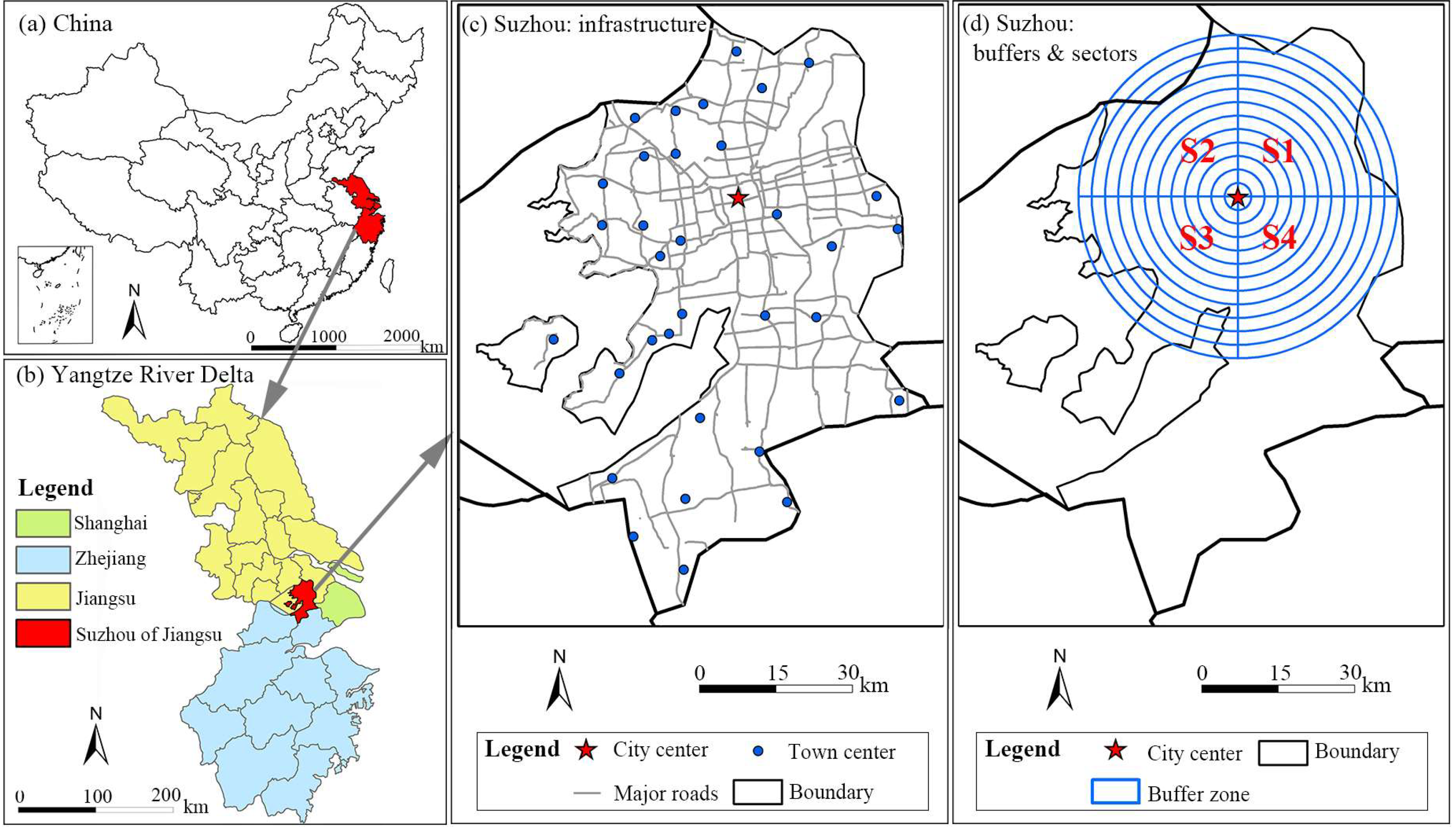
2.1. Study Area and Datasets

Suzhou is the most economically developed city located in the southeastern part of the Jiangsu Province in Eastern China (Figure 1a,b). It is one of the central cities in the Yangtze River Delta, urban agglomeration, and is adjacent to China’s economic center, Shanghai. Suzhou has five administrative districts (Gusu, Xiangcheng, Wuzhong, Huqiu, and Wujiang) and four satellite cities (Changshu, Kunshan, Zhangjiagang, and Taicang). Our study area includes the above five districts that total 2,778 km² (Figure 1c,d; denoted as Suzhou, hereafter).

Suzhou has a subtropical monsoon marine climate with four distinct seasons, abundant rainfall, and rich water resources [49], facilitating cropping and noncommercial vegetation growth. The superior geographical location and good climate have led to early industrialization and urbanization in Suzhou, as compared to other Chinese cities. The built-up area has increased from 12.1% in 2000 to 40.3% in 2015 [49], attributed to the rapid development of the economy and urban infrastructure. Such rapid urbanization has claimed much ecological and agricultural land and led to a decline in vegetation coverage. Industrialization, urbanization, and vegetation decline has affected the local climate substantially, and areas affected by SUHI have expanded significantly [50].

We used seven Landsat images (

Table 1. Landsat images for LST derivation—satellite, sensor, cloud, date, season, and usage.

Satellite	Sensor	Date	Season	Cloud (%)	Usage
Landsat-5	TM (30m)	01 May, 1996	Spring	0.0	Derive LST and land coverage indices
Landsat-5	TM (30m)	05 Aug, 1996	Summer	0.4	Derive LST, land coverage indices, and land-use pattern
Landsat-5	TM (30m)	04 Mar, 2004	Spring*	0.1	Derive LST and land coverage indices
Landsat-5	TM (30m)	23 May, 2004	Spring*	0.0	Derive LST and land coverage indices
Landsat-5	TM (30m)	26 Jul, 2004	Summer	0.0	Derive LST, land coverage indices and land-use pattern
Landsat-8	OLI (30m) TIRS (30m)	22 Apr, 2016	Spring	0.2	Derive LST and land coverage indices
Landsat-8	OLI (30m) TIRS (30m)	27 Jul, 2016	Summer	6.4	Derive LST, land coverage indices and land-use pattern

Note: The date of available spring images in 2004 cannot well match those in 1996 and 2016, we therefore assembled two Landsat images in March and May 2004 and produced their average LST to reflect the thermal patterns in spring 2004.

) to derive the spring and summer LST patterns and land coverage indices, and applied vector-based maps (

Table 2. Vector datasets for proximity layers—scale, feature, date, and usage.

Map	Scale	Feature	Date	Usage
Administrative map	1:1,000,000	Boundary, city center, and town centers	2016	Extract proximity layers
Road network map	1:1,000	OSM major roads	1996, 2004, 2016	Extract proximity layers

) to define the administrative boundary and generate the spatial driving factors. All Landsat images were provided by Geospatial Data Clouds and these are the best images of Suzhou that could be used for the LST retrieval and further comparison, considering the negative effects of cloud and cloud shadow. LST derivation and the calculation of the built-up area, vegetation, and water, were performed using these images. The administrative map was collected from the Geographical Information Monitoring Cloud Platform (GIMCP) and was employed to define administrative boundaries, the Suzhou City center (hereafter denoted as the city center), and town centers. The road network maps were collected from the Open Street Map (OSM) and were used to define major roads in 1996, 2004, and 2016. All vector maps were used to extract proximity factors, such as distance to the city center, town centers, and major roads, representing the spatial accessibility to urban facilities.

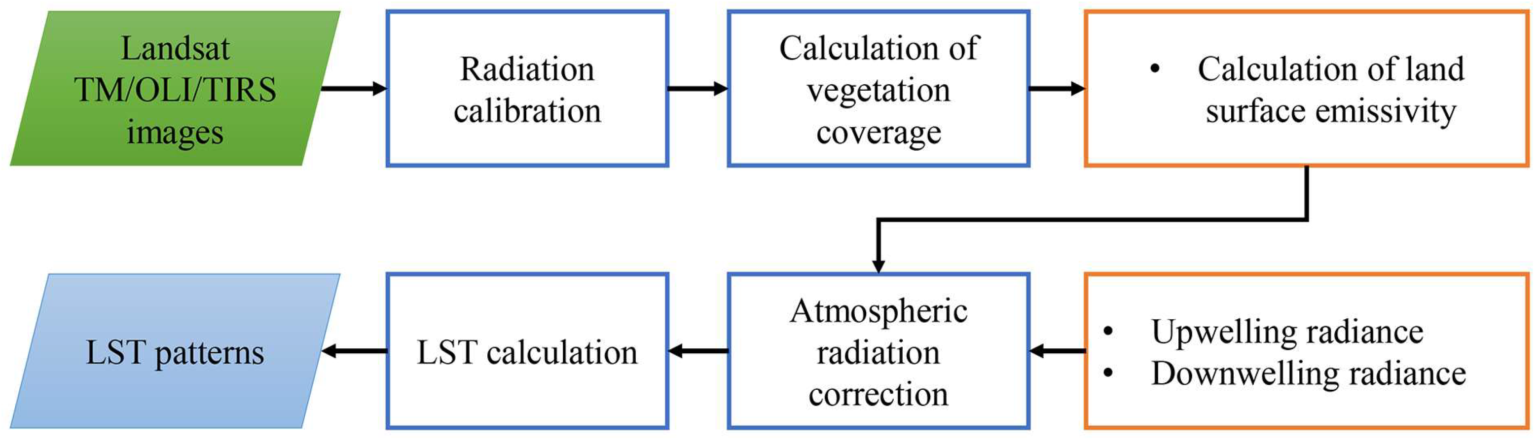
2.2. LST Retrieval Method

Before LST retrieval, we performed atmospheric correction of the reflective band observations for the selected Landsat images. Practically, we applied “Radiometric Calibration” and “FLAASH Atmospheric correction” tools in ENVI 5.4, to convert Landsat digital numbers to exoatmospheric reflectance. These reflective bands were used to produce land coverage indices and land-use patterns.

LST at Suzhou was derived using the Landsat-5 TM thermal band-6 and Landsat-8 TIRS band-10, based on the radiative transfer equation, as described in early publications [38,51]. The thermal infrared radiation $L_{sens}\left(\lambda \right)$ can be given by [38,51]:

$$L_{sens}\left(\lambda \right)=\left({\epsilon }_{\lambda }·B_{\lambda }\left(TS\right)+\left(1-{\epsilon }_{\lambda }\right)·L_{\lambda }\downarrow \right)·{\tau }_{\lambda }+L_{\lambda }\uparrow$$

(1)

where $\lambda$ denotes the wavelength, ${\epsilon }_{\lambda }$ denotes the land surface emissivity, $TS$ denotes the real temperature of the land surface, $B_{\lambda }\left(TS\right)$ denotes the Planck’s law, ${\tau }_{\lambda }$ denotes the total atmospheric transmissivity, $L_{\lambda }\uparrow$ denotes the upwelling radiance, and $L_{\lambda }\downarrow$ denotes the downwelling atmospheric radiance.

The LST derivation procedure (Figure 2) includes four major steps. (1) A radiation calibration is performed then the land coverage for vegetation, urban area, soil, and water is calculated; (2) land surface emissivity is calculated, based on the radiance ratio between a natural object and a blackbody; (3) atmospheric radiation correction is performed by inputting the land surface emissivity, and upwelling, and downwelling radiances that were retrieved using the Atmospheric Correction Parameter Calculator (atmcorr.gsfc.nasa.gov), and (4) LST is calculated using an inverse Planck law, based on thermal radiation of the blackbody, and finally the LST spatial patterns are visualized.

2.3. Selected Influencing Factors

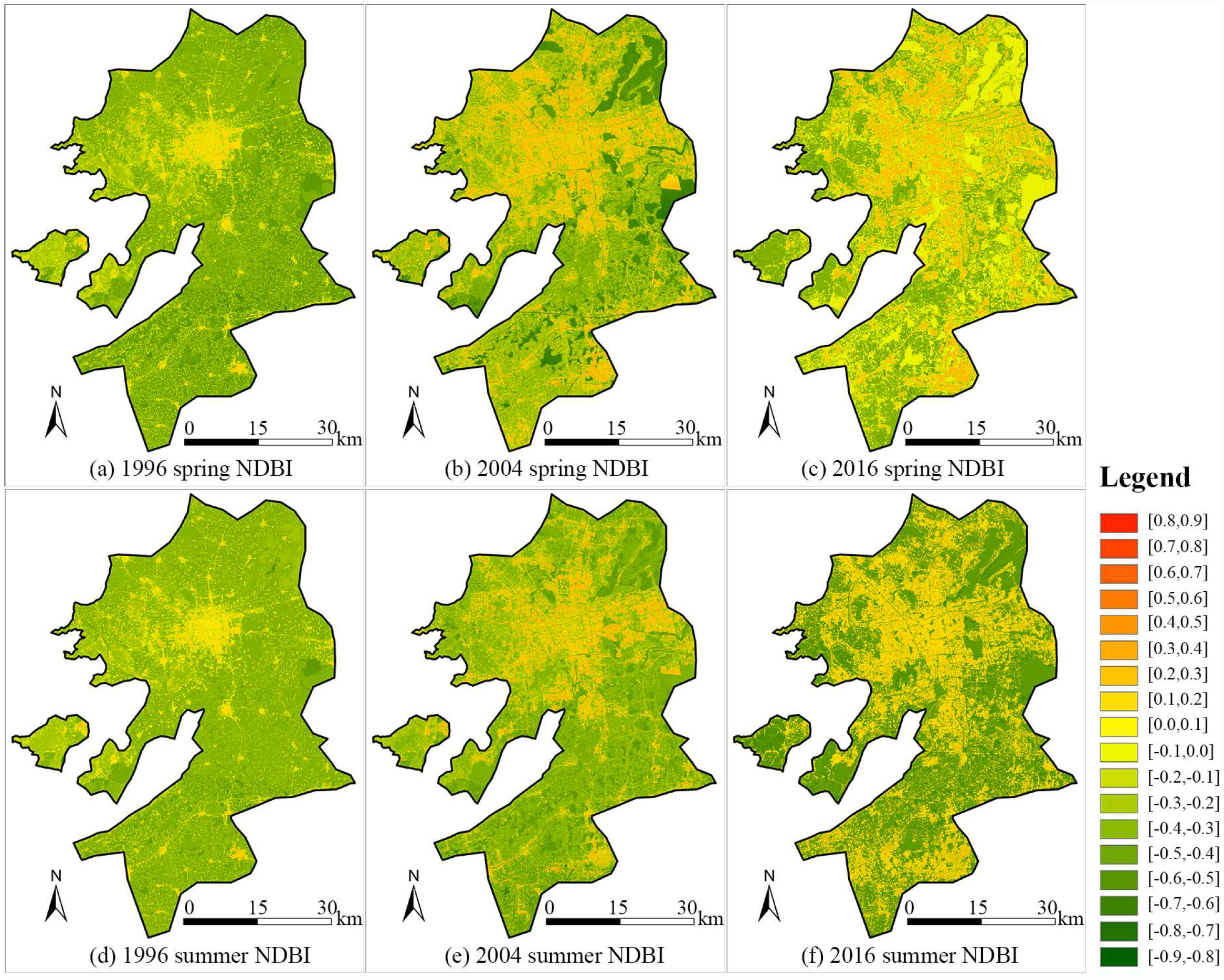
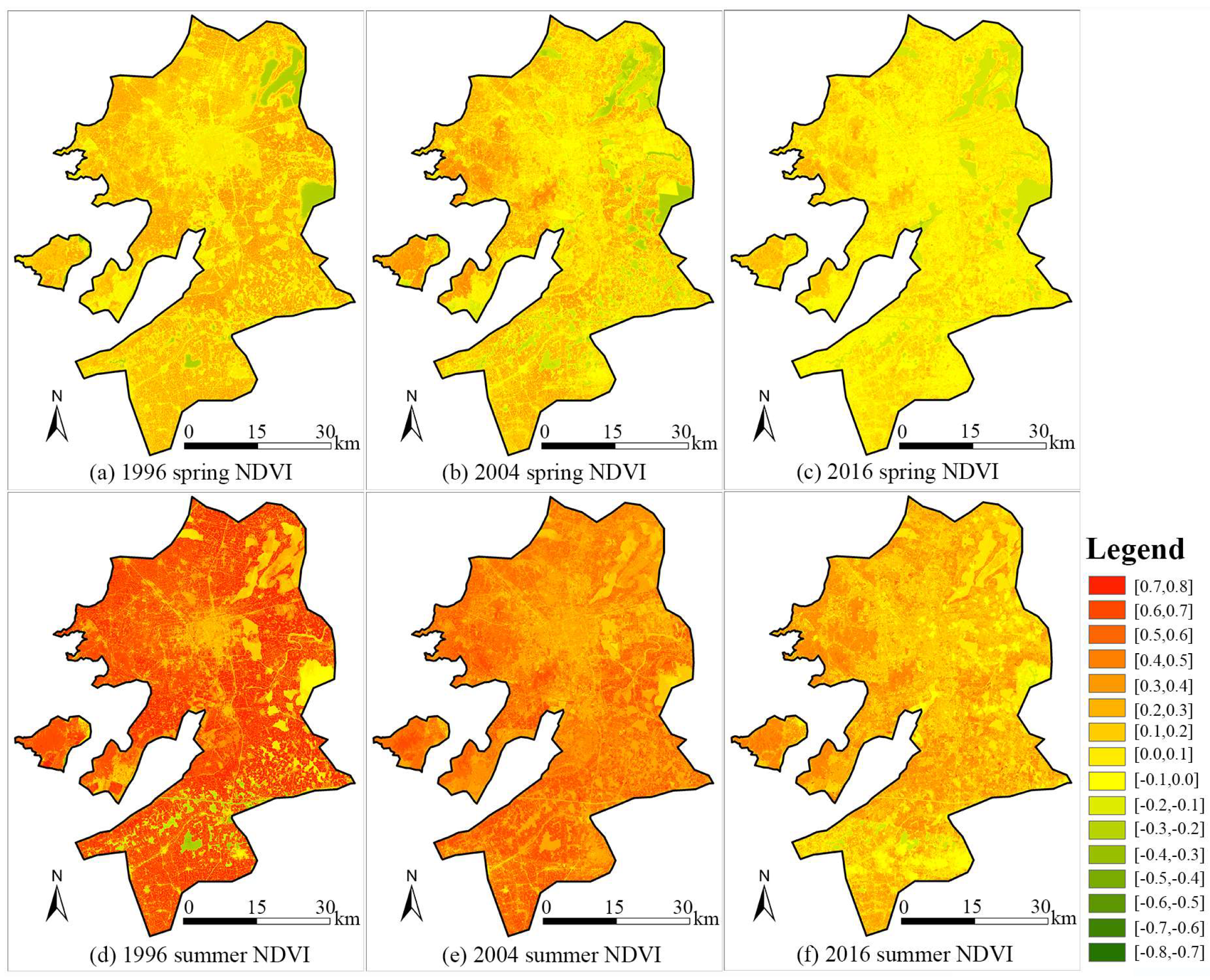
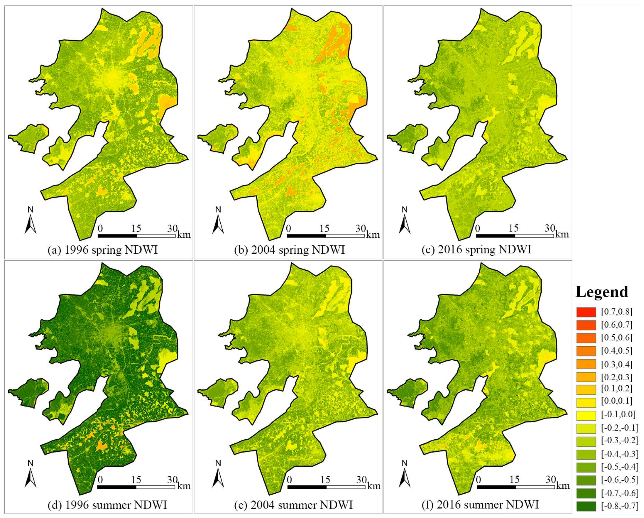
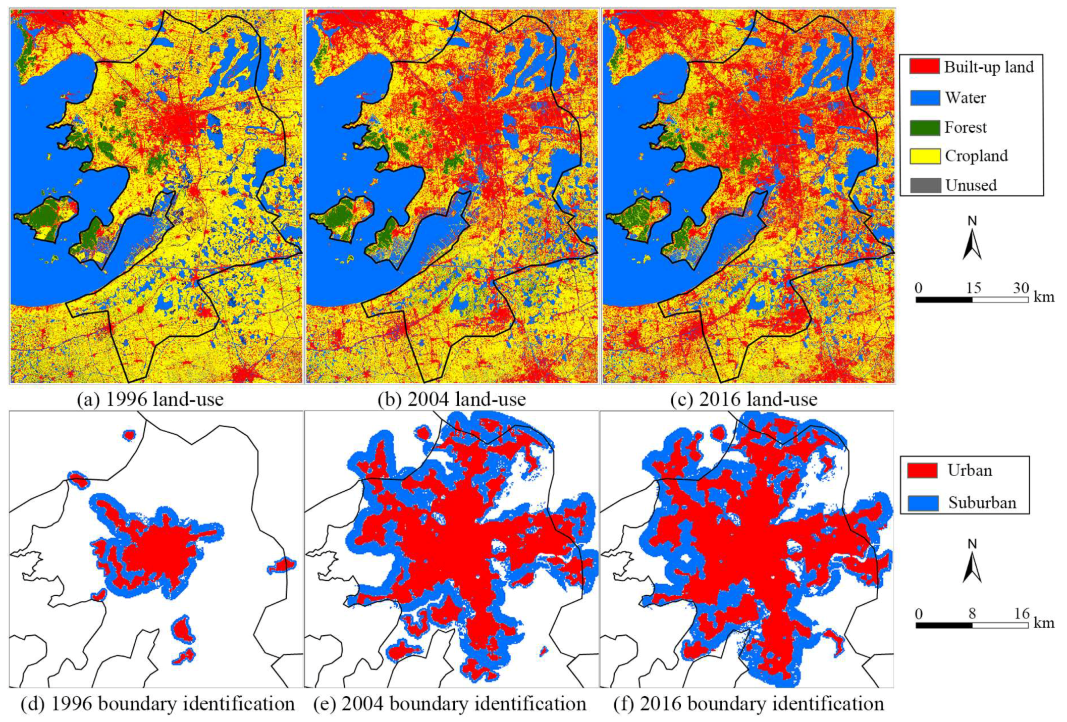
2.3.1. Land Coverage: NDBI, NDVI, and NDWI

NDBI is an urban impervious surface index that represents the intensity of the urban built-up area and is an important analytical tool in characterizing land development, urbanization, and land surface parameters [36]. NDVI is a live green vegetation indicator, reflecting the vegetation coverage by separating vegetation from water and soil [52]. NDWI is a liquid water metric that denotes the coverage of water bodies and land water content [53]. The NDBI, NDVI, and NDWI calculations were performed using the Band Math tool in ENVI 5.4. The three indices were calculated as [54]:

$$\{\begin{array}{l}NDBI=\frac{SWIR-NIR}{SWIR+NIR}\\ NDVI=\frac{NIR-R}{NIR+R}\\ NDWI=\frac{Green-NIR}{Green+NIR}\end{array}$$

(2)

where SWIR denotes the short-wave infrared band, NIR denotes the near-infrared band, R denotes the red band, and Green denotes the green band. For calculating the indices using Landsat imagery, this can be rewritten as:

$$\{\begin{array}{c}NDBI~\frac{Band5-Band4}{Band5+Band4}\left(TM/ETM+\right)~\frac{Band6-Band5}{Band6+Band5}\left(OLI\right)\\ NDVI~\frac{Band4-Band3}{Band4+Band3}\left(TM/ETM+\right)~\frac{Band5-Band4}{Band5+Band4}\left(OLI\right)\\ NDWI~\frac{Band2-Band4}{Band2+Band4}\left(TM/ETM+\right)~\frac{Band3-Band5}{Band3+Band5}\left(OLI\right)\end{array}$$

(3)

Figure 3 shows that the high NDBI was distributed principally in the city center, but over time the areas with high NDBI expanded from the city center to the urban fringe; meanwhile, there were no substantial differences in the NDBI, between spring and summer. Figure 4 shows that there was a decrease in NDVI, over time, and the NDVI was higher in summer than in spring. Figure 5 shows that the broad waters at Suzhou were distributed in the eastern and southern regions, and the spatial patterns of NDWI differed between spring and summer, and among the three years.

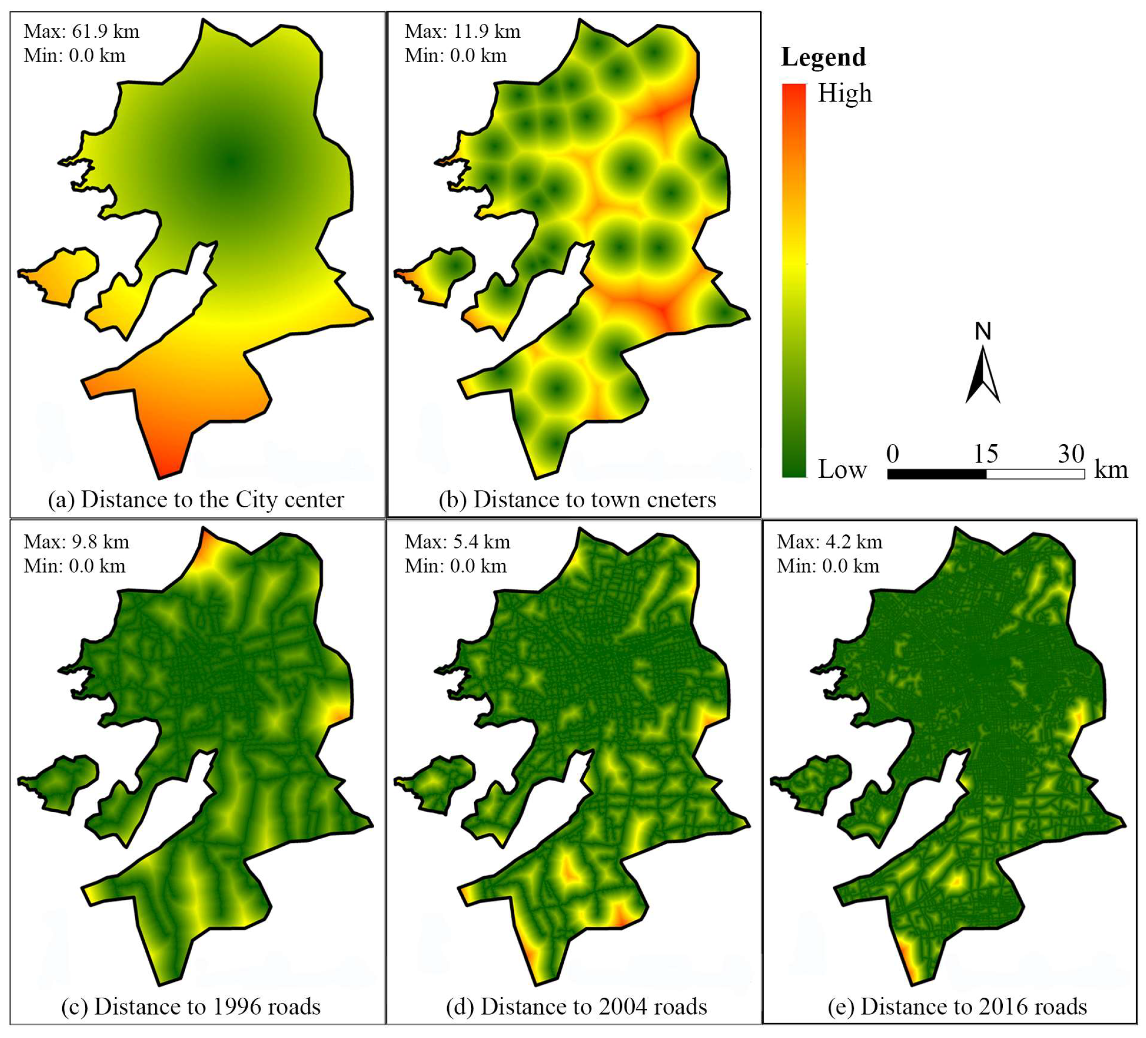
2.3.2. Distance-Based Proximity Factors

We applied the vector datasets (see Table 2) to extract the proximity factors to address the influence of distance to city center (D-city), town centers (D-town), and major roads (D-road), for each year. Maps of these spatial factors were produced using the ArcGIS 10.2 Euclidean distance tool, with all factors measured in kilometers (Figure 6). The lower values of these proximity factors are found near centers and roads, because the proximity was calculated using an inverse distance weight. The D-city maximum is about 62 km, occurring to the south of Suzhou, and the D-town peak is about 12 km, much shorter than D-city. Due to the road network construction in Suzhou, the length and density of road networks increased during the past two decades, leading to a decrease in the maximum D-road from ~10 km in 1996 to ~5 km in 2004, and then to ~4 km in 2016.

LST is a land surface parameter that is spatially heterogeneous, which implies that it may be strongly correlated with spatial coordinates [55]. We therefore incorporated both longitude (D-X) and latitude (D–Y), as additional spatial influencing factors, in exploring their effects on LST at Suzhou.

2.4. Analysis Methods

SUHIs are caused by artificial heat, heat storage of artificial constructions, and reduction of green space. At local and regional scales, Landsat-derived LST has been widely applied to examine SUHI variation [15], which in turn reflect the impacts of changing LST on the environments. SUHIs can be defined based on an LST classification that can be performed using an urban–suburban boundary method [15,56,57]. The terrain’s effect on the SUHI intensity was not considered in this research, because our study area was very flat [57]. We computed SUHI intensity ($\Delta \mathrm{T}$) by [58]:

$$\Delta \mathrm{T}=LS{T}_{urban}-LS{T}_{suburban}$$

(4)

where $LS{T}_{urban}$ is the mean LST of urban areas and $LS{T}_{suburban}$ is mean LST of the suburban area.

We followed Zhou et al. [56] to define the urban area each year, using the segmentation of the built-up density map, which was produced using a moving 1km×1km grid. The segmentation threshold for urban identification was 0.5 at Suzhou, for all three years, where the suburban area was taken as the same size as the urban area (Figure 7). We followed Meng et al. [57] to define the SUHI level (

Table 3. Surface Urban Heat Island (SUHI) classification criteria at Suzhou [57].

Level	Temperature Range	Calculation Method
I	Low temperature	LSTsuburban ≤ LSTori < (LSTsuburban + ∆T)
II	Sub-low temperature	(LSTsuburban + ∆T) < LSTori < (LSTsuburban + 2∆T)
III	Middle temperature	(LSTsuburban + 2∆T) < LSTori < (LSTsuburban + 3∆T)
IV	Sub-high temperature	(LSTsuburban + 3∆T) < LSTori < (LSTsuburban+4∆T)
V	High temperature	LSTori ≥ (LSTsuburban + 4∆T)

Note: LST_ori is the LST of each pixel, for each season, each year.

), which has five grades, to show the temperature range and SUHI at Suzhou.

We used GAM to examine the relationship between LST and its potential influencing factors. As an extension of a generalized linear model, GAM connects LST with all factors, using smoothing functions, where the factors are added into the model, one by one. The GAM can be given by [59]:

$$E\left[Y|X\right]=G\left(\alpha +\sum _{i=1}^d{f}_i\left(X^i\right)\right)$$

(5)

where E is the expected value, Y is the dependent variable, X are the independent variables, G is a connect function, α is the linear error, d is the number of independent variables, and f_i is the smoothing function. Using specific parameters, Equation (5) can be expressed as:

$$\begin{gathered} LST~\mathrm{s}\left(NDBI\right)+\mathrm{s}\left(NDVI\right)+\mathrm{s}\left(NDWI\right)+\mathrm{s}\left(D-city\right)+\mathrm{s}\left(D-town\right)+\mathrm{s}\left(D-road\right) \\ +\mathrm{s}\left(D-X\right)+\mathrm{s}\left(D-Y\right)+\epsilon \end{gathered}$$

(6)

where LST is the dependent variable (LST); s is a natural cubic spline smoothing; NDBI, NDVI, NDWI, D-city, D-town, D-road, D-X and D–Y are the spatial influencing factors; and ε is an error term.

GAM generates two statistics [10,48]—the accumulated deviance explained (ADE) and the Akaike information criterion (AIC) when examining the relationships between LST and influencing factors. ADE reports how much the independent variables explain the dependent variable (LST) regarding the modeling residual deviance [59]. AIC measures the relative quality of the model and is inversely proportional to the fitting performance. A smaller AIC suggests a better model [10]. GAM is a stepwise model that incorporates the independent variables, one by one, by which the ADE and the AIC collaboratively determine the rank-order of each variable. Anterior variables yield stronger effects while posteriors yield weaker effects. In Equation (6), the rank-order of the driving factors was arranged by the categories presented in Section 2.3, but this would be different when inputting real samples. GAM was implemented using the R-Gui package “mgcv”.

3. Results

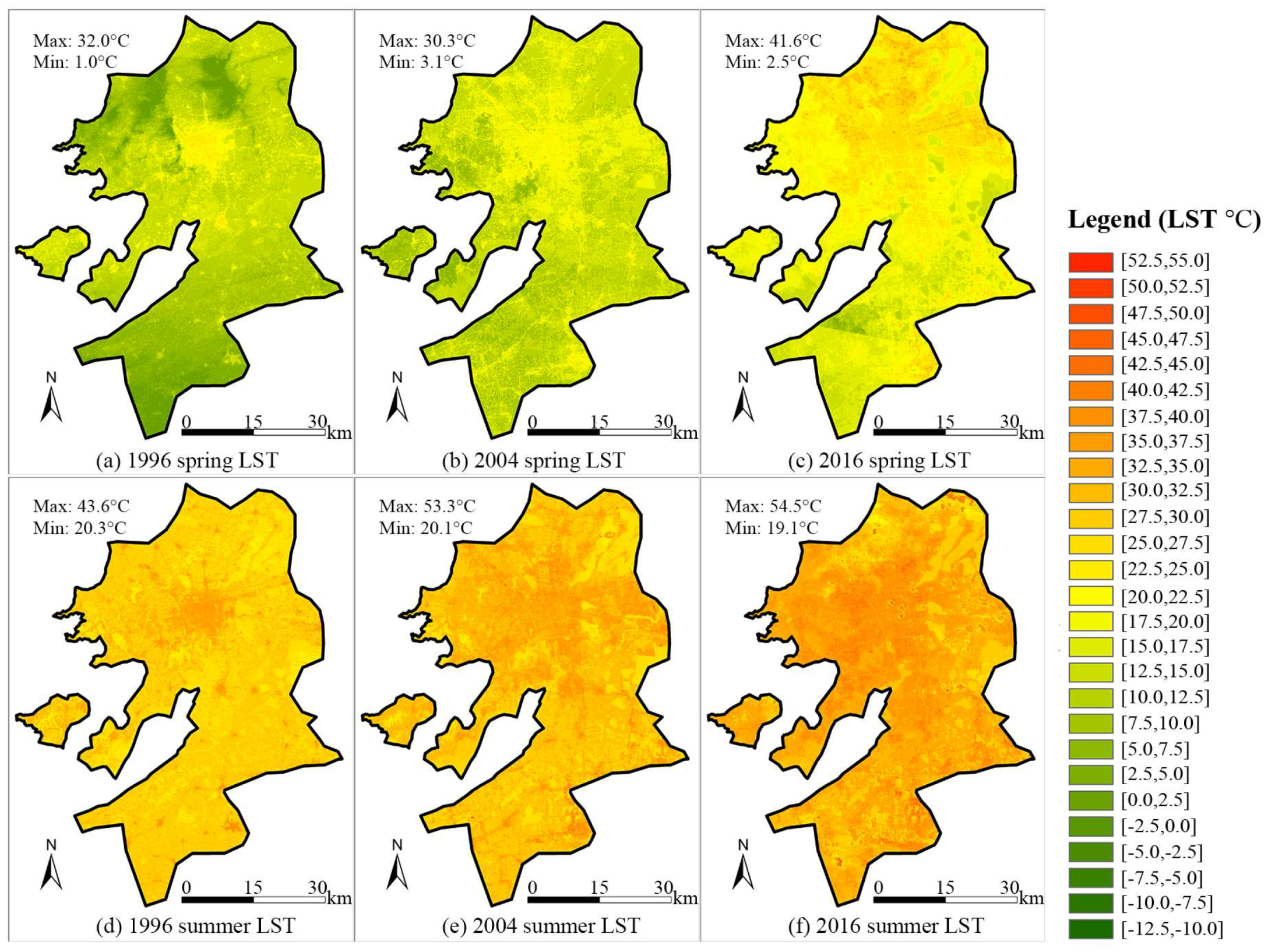
3.1. Spring and Summer LST

LST at Suzhou was derived using the radiative transfer equation, based on the near-infrared bands of Landsat images [60,61,62]. We calculated vegetation coverage and land surface emissivity for atmospheric radiation correction [63,64], and converted surface heat radiation intensity to LST [65,66]. We derived the spring LST data (Figure 8a–c) using the method presented in Section 2.2 and used the summer LST data (Figure 8d–f), reported by an earlier publication [38] on the Taihu Lake Basin.

The LST maps clearly show that the warmest regions lie in and near the city center and have expanded in spatial extent, with urban growth (Figure 8).

Table 4. The summary statistics of spring and summer LST at Suzhou in 1996, 2004, and 2016.

Year	Season (°C)	Min (°C)	Max (°C)	Range (°C)	Mean (°C)	SD
1996	Spring	1.00	32.00	31.00	11.09	4.62
	Summer	20.30	43.55	23.26	28.28	2.56
2004	Spring	3.13	30.30	27.17	14.46	3.67
	Summer	20.12	53.31	33.19	30.72	3.12
2016	Spring	2.48	41.59	39.11	20.63	4.35
	Summer	19.07	53.89	34.82	33.95	3.69

shows that, for spring 1996, 2004, and 2016, the lowest LST decreased by about 1~2 °C, but the highest LST significantly increased by about 10 °C; for summer, the lowest LST decreased slightly by ~1 °C, but the highest LST increased significantly by ~10.5 °C. The mean LST values show that Suzhou became warmer with time, rising by ~0.5 °C in spring per year and by ~0.3 °C in summer per year, suggesting a faster warming in spring than in summer. Except for spring 1996, the range and standard deviation of LST increased with time, suggesting greater LST differences, across space and time.

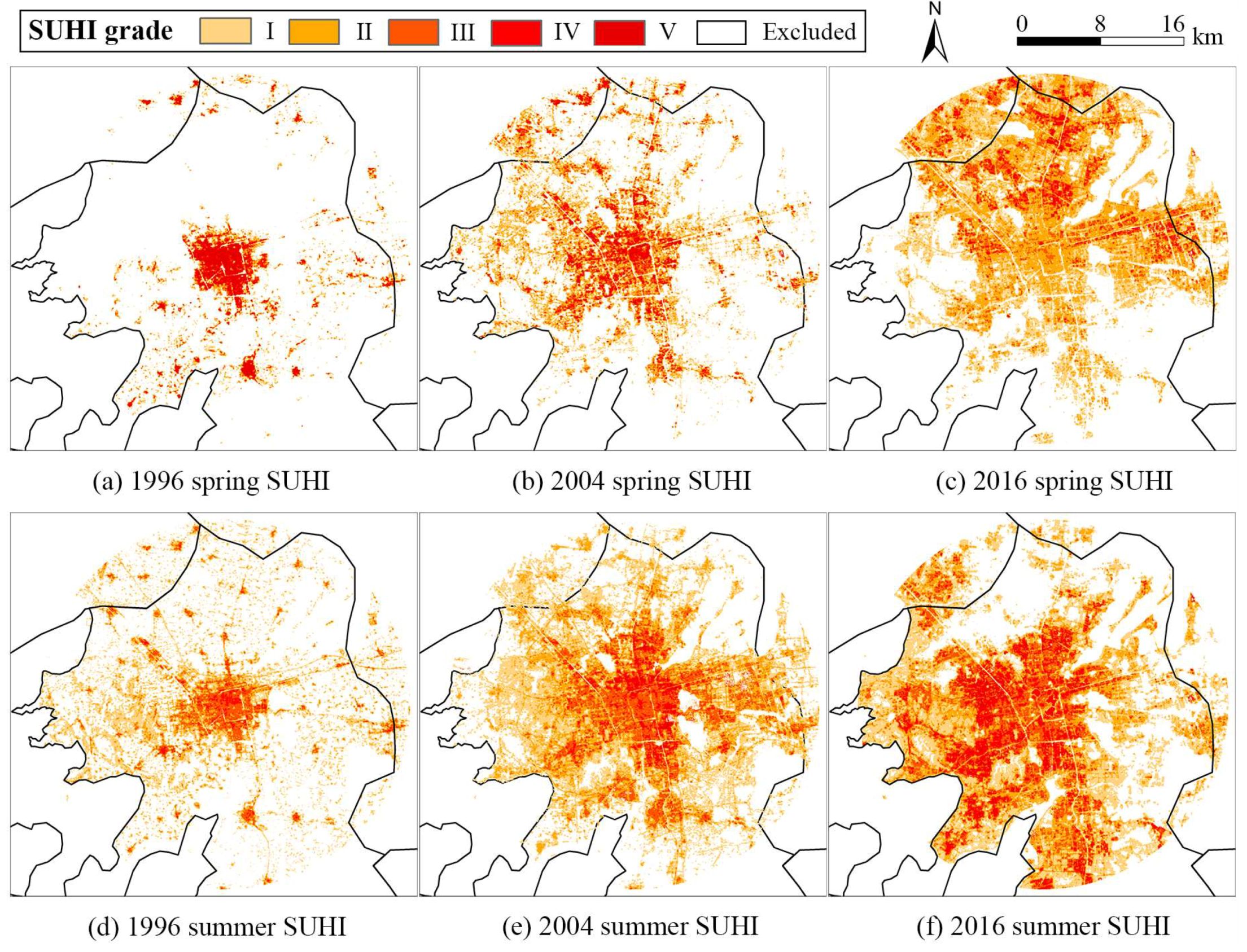
3.2. Spring and Summer SUHI

Table 5. Mean LST and SUHI intensity (ΔT) for spring and summer 1996, 2004, and 2016.

Season	1996			2004			2016
	LSTurban	LSTsuburban	ΔT	LSTurban	LSTsuburban	ΔT	LSTurban	LSTsuburban	ΔT
Spring	4.73	3.58	1.15	7.06	5.87	1.19	22.84	20.52	2.32
Summer	19.80	17.91	1.89	25.26	21.99	3.27	41.37	37.77	3.60

shows increasing SUHI intensity (ΔT) over time, and stronger SUHI intensity in summer than in spring. Figure 9 shows clear increases in the areas with high temperature (strong SUHI effect), for both spring and summer, across the three years, and shows a different spatial distribution of SUHI intensity between these two seasons. For all three years, Figure 9 also shows larger areas that were affected by SUHIs, in summer than in spring. Specifically, the area in spring increased from 223 km² in 1996 to 626 km² in 2004, and to 1116 km² in 2016; meanwhile, the area in summer increased from 556 km² in 1996 to 1170 km² in 2004, and to 1295 km² in 2016. These indicate a substantial warming trend associated with the rapid urban growth and drastic land-use change, across the study area.

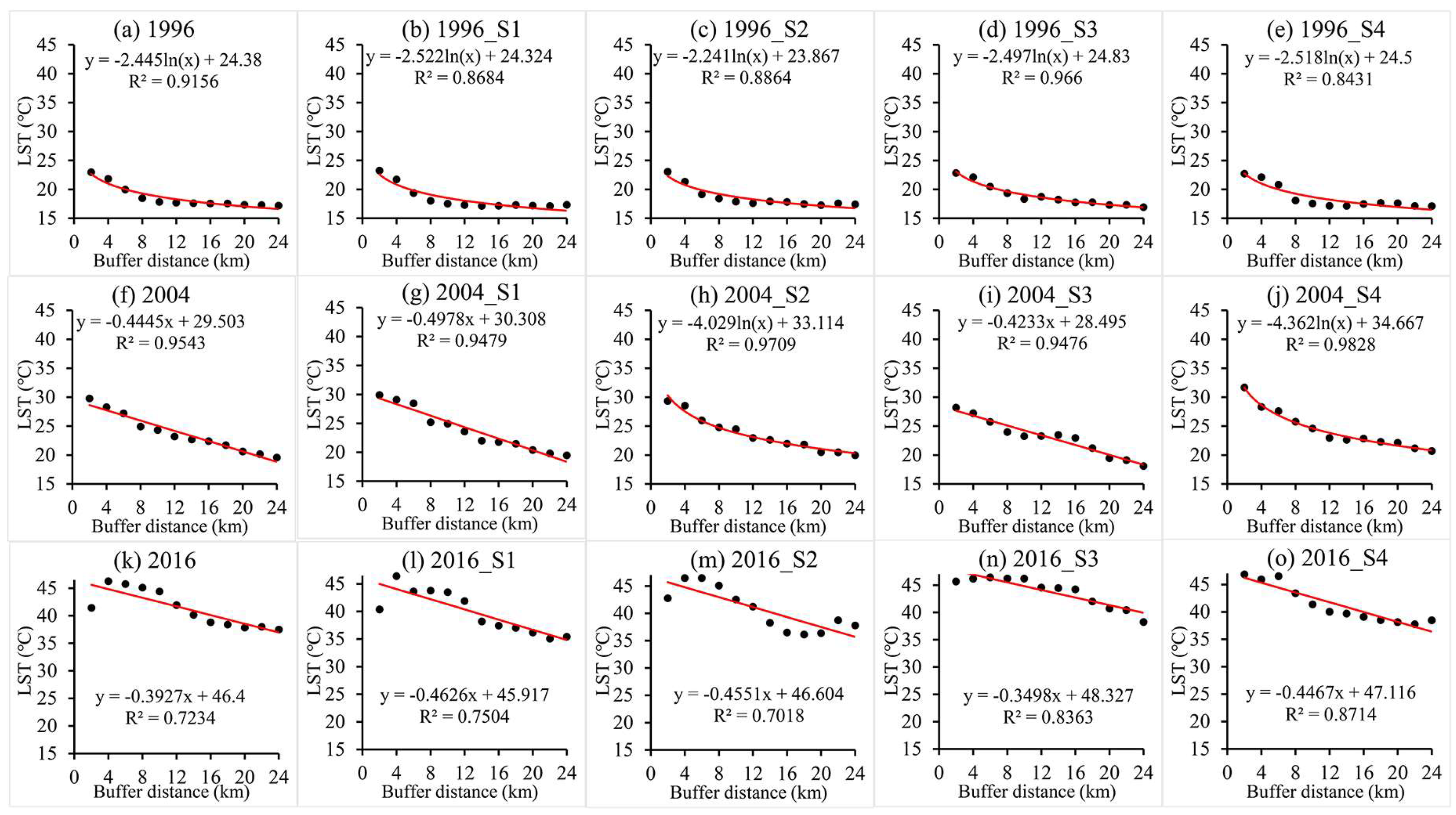
3.3 LST Gradients in 1996, 2004, and 2016

Based on the sector layout in Figure 1d, we examined the relationships between LST and the distance to the city center, then presented the curves with the highest R²s (Figure 10 and Figure 11). Clear decreases in LST were detected in both spring and summer, for all three years.

The distribution of LST at Suzhou, varied over time, and the spatiotemporal changes in LST were highly affected by proximity to the city center (Figure 10 and Figure 11). In 1996, both spring and summer followed logarithmic functions, for all four sectors, suggesting that LST decayed with the distance to the city center. In 2004, both spring and summer followed the logarithmic functions for S2 and S4, and followed linear functions for S3; however, for S1, spring followed a logarithmic function while summer followed a linear function. These suggest that the relationships between LST and the distance to the city center were more complex in 2004 than in the other two years. In 2016, all sectors followed linear functions, where S3 decreased most rapidly in spring but least rapidly in summer, as inferred by the slopes. In 1996, 2004, and spring 2016, the city center was the warmest location for all sectors; in summer 2016, the city center was not the warmest location for S1, S2, and S3 (Figure 11). These may be due to the impact of cloud in the city center and the relatively low LST in S4, where nearly half were excluded in the SUHI because they did not belong to any SUHI levels (Figure 9f).

3.4 Factor Effects on LST

The GAMs show that the AIC decreased when more factors were included in the models. The factors explained more than 75% of the ADEs for spring and explained more than 54% of the ADEs for summer, when all eight factors were included in the GAMs (

Table 6. Generalized additive models (GAMs) linking LST and its influencing factors in 1996, 2004, and 2016.

Season	Rank	1996			2004			2016
		Driving Factor	ADE (%)	AIC	Driving Factor	ADE (%)	AIC	Driving Factor	ADE (%)	AIC
Spring	1	+D-Y	51.3	6427.71	+NDVI	61.9	5526.43	+D-Y	46. 6	6465.20
	2	+NDBI	63.7	6075.16	+D-Y	76.0	4967.77	+NDWI	67.2	5874.43
	3	+NDWI	69.1	5881.10	+NDBI	82.2	4613.61	+NDBI	78.4	5373.09
	4	+D-X	72.7	5752.56	+NDWI	83.1	4552.96	+D-X	81.6	5188.70
	5	+D-city	74.6	5673.85	+D-city	83.7	4518.78	+D-city	83.2	5090.98
	6	+NDVI	75.5	5648.72	+D-town	84.0	4508.96	+D-road	84.3	5021.60
	7	+D-road	75.8	5637.41	+D-X	84.3	4494.06	+D-town	85.0	4981.46
	8	+D-town*	75.8	5638.24	+D-road	84.3	4495.68	+NDVI	85.4	4952.90
Summer	1	+NDBI	42.3	5110.99	+NDBI	56.3	5315.95	+NDWI	18.3	6566.45
	2	+NDWI	50.3	4943.03	+NDWI	59.0	5247.30	+NDVI	36.5	6263.40
	3	+D-city	53.7	4869.08	+NDVI	62.9	5139.85	+D-Y	45.0	6101.55
	4	+NDVI	55.8	4813.21	+D-X	64.1	5112.77	+D-X	47.9	6045.81
	5	+D-Y	56.4	4807.30	+D-city	64.9	5091.08	+NDBI	50.3	5996.70
	6	+D-X	57.4	4787.89	+D-Y	65.5	5079.15	+D-town	51.6	5973.33
	7	+D-road	58.1	4776.39	+D-road	65.8	5070.68	+D-road	52.9	5945.46
	8	+D-town*	58.2	4775.86	+D-town	65.9	5058.02	+D-city	54.2	5931.15

Note: For both spring and summer 1996, D-town was not statistically significant, showing that this factor was not correlated with LST in 1996. The inclusion of D-town could not improve, and even reduced, the GAM performance for 1996. We, therefore, excluded D-town in analyzing the 1996 LST.

). This suggests that these factors yield a stronger ability in explaining the LST distribution in spring, than in summer. The effects of the selected factors on LST vary with time, as inferred by the factor rank-order. Note that rank-order is determined, based on both the ADE and AIC, regardless of their positive or negative effects on the SUHIs.

For spring, the D-Y (horizontal direction) factor substantially affected the LST distribution but was less influential in summer 1996, 2004, and 2016. Regarding the positional factors, except for summer 2004, the D-Y (horizontal direction) was more influential than the D-X (vertical direction). For summer, NDBI was the most influential factor for LST in 1996 and 2004, but had a significantly decreased influence on LST, in 2016. For both spring and summer, the land coverage indices were more influential than the spatial proximity factors. For spring, D-city produced a stable effect on LST in spring but only ranked fifth, while in summer this factor produced a less important role in contributing to SUHIs (

Table 7. Spring LST change in response to the spatial influencing factors. A negative correlation between LST and the proximity factors suggests an intensifying effect on SUHIs, while a negative correlation between LST and the other types suggests a mitigating effect on SUHIs.

Driving Factor	Year	Interval and Trend				Effect
		Interval	Trend	Interval	Trend
NDBI	1996	> −0.4*	↗			Monotonous
	2004	> −0.3*	↗			Monotonous
	2016	−0.3*–0.0	↗↗	> 0.0	↗	Piecewise
NDWI	1996	−0.4*–0.0	↗	> 0.2	↘	Piecewise
	2004	−0.3*–0.1	↘	> 0.1	↘↘	Piecewise
	2016	> −0.4*	↘			Monotonous
NDVI	1996	> −0.23*	↘			Piecewise
	2004	> −0.3*	↘			Monotonous
	2016	> 0.0	↘			Monotonous
D-road	1996	> 0 km	↘			Monotonous
	2004	> 0 km	↘			Monotonous
	2016	> 0 km	↘			Monotonous
D-city	1996	0–10 km	↘	> 10 km	↗	Piecewise
	2004	0–10 km	↘	> 10 km	↗	Piecewise
	2016	0–25 km	↘	> 25 km	↗	Piecewise
D-town	1996					Not significant
	2004	> 0 km	↗			Monotonous
	2016	0–2 km	↘	> 2 km	↗	Monotonous

Note: “↗” denotes a positive correlation, “↗↗” denotes a strong positive correlation, “↘” denotes a negative correlation, and “↘↘” denotes a strong negative correlation. An asterisk “*” denotes that these values are the minima of the corresponding factors.

). For 1996, the LST did not yield a statistically significant correlation with D-town, while in 2004 and 2016 there were weak correlations between them. The D-road factor produced a weak and varying effect on LST for spring, but yielded a weak and stable effect on LST for summer.

We further identified intervals of factor values and the trends affecting LST, based on GAM plots that reflected the relationships between LST and each influencing factor. Eighteen items were included in both Table 7 and

Table 8. Summer LST change in response to the spatial influencing factors. A negative correlation between LST and the proximity factors suggests an intensifying effect on the SUHIs, while a negative correlation between LST and the other types suggests a mitigating effect on the SUHIs.

Driving Factor	Year	Interval and Trend						Effect
		Interval	Trend	Interval	Trend	Interval	Trend
NDBI	1996	> −0.60*	↗					Monotonous
	2004	−0.3–−0.2	↘	−0.2–−0.15	↗↗	> −0.15	↗	Piecewise
	2016	> −0.33*	↗					Monotonous
NDWI	1996	> −0.70*	↘					Monotonous
	2004	> −0.43*	↘					Monotonous
	2016	> −0.52*	↘					Monotonous
NDVI	1996	> −0.25*	↘					Monotonous
	2004	0–0.1	↗	> 0.1	↘			Piecewise
	2016	> −0.1*	↘					Monotonous
D−road	1996	> 0 km	↘					Monotonous
	2004	> 0 km	↘					Monotonous
	2016	> 0 km	↘					Monotonous
D−city	1996	0–10 km	↘	> 10 km	↗			Piecewise
	2004	0–30 km	↘	> 30 km	↗			Piecewise
	2016	0–40 km	↘	> 40 km	↗			Piecewise
D−town	1996							Not significant
	2004	> 0 km	↗					Monotonous
	2016	0–3 km	↘	> 3 km	↗			Piecewise

, with six spatial influencing factors in each of the three years. For spring, ten of these items illustrated monotonous correlations between LST and the factors, while the other seven items illustrated piecewise correlations; for summer, eleven of these items illustrated monotonous correlations, while the other six items illustrated piecewise correlations. Compared to monotonous correlations, piecewise correlations suggest more complex relationships between LST and the factors.

NDBI was positively correlated with LST, in most cases, but was correlated, piecewise, with LST in spring 2016 and summer 2004. This factor clearly showed an intensifying effect on the SUHIs at Suzhou. For spring 2016, the positive correlations had two pieces with a critical point at 0.0 (Table 7), where NDBI in the [−0.3, 0.0] range was primarily associated with water bodies, agricultural land, and forest, and NDBI greater than 0.0 was primarily associated with rural residential land and built-up urban areas. For summer 2004, the LST–NDBI relationships had three pieces with two critical points at −0.2 and −0.15 (Table 8). The [−0.3, −0.2] NDBI range was primarily associated with water bodies, agricultural land, and forest, the [−0.2, −0.15] NDBI range was primarily associated with rural residential land, and an NDBI greater than −0.15 was primarily associated with built-up urban areas. As shown by Figure 3, the built-up urban areas in the city center did not maintain the same NDBI values across the years, leading to varying effects on the SUHIs. NDWI was correlated, piecewise, with LST in spring 1996 and 2004, where NDWI in the [−0.4, 0.0] range corresponded to the rural residential land and built-up urban areas; for the other time-points, this index was monotonously, negatively correlated with LST. These indicate that NDWI was basically a mitigating factor for the SUHIs at Suzhou. NDVI between 0.0–0.1 showed a positive correlation with LST in summer 2004, but showed monotonously negative correlations with LST, in other cases. This demonstrated that a higher NDVI linked to a lower LST, and NDVI yielded a significant mitigating effect on the SUHIs at Suzhou.

D-road was negatively correlated with LST, for both spring and summer, in all three years. This suggests that areas closer to major roads were linked with a higher LST, denoting an increased effect of D-road on the SUHIs. There were complex correlations between D-city and LST because both seasons, in all three years, yielded piecewise intervals and trends. Within 10 km from the city center, D-city had a clear intensifying effect on the SUHIs for spring 1996 and 2004, and summer 1996; within 30 km and 40 km from the city center, the factor also showed a clear intensifying effect on the SUHIs, for summer 2004 and 2016, respectively. When D-city was greater than these critical distances, this factor had a lesser effect on LST (Table 7 and Table 8). The increasing critical distance of D-city implied the spatial expansion of SUHIs at Suzhou, accompanied by its urban growth, leading to the increased effect of the city center on the SUHIs. D-town showed a mitigating effect on the SUHIs, for both spring and summer 2004; whereas, for 2016, this factor intensified the SUHIs within 2–3 km but mitigated the SUHIs when D-town was greater than the critical distance. The increasing critical distance of D-town from 2004 to 2016 indicated the expansion of the built-up areas in town centers and the increased effect of the town centers on the SUHIs.

4. Discussion

We used Landsat imagery to derive LST patterns and generate SUHIs at Suzhou, for spring and summer 1996, 2004, and 2016. The warmest regions lay in and near the city center, and had expanded in spatial extent, with urban growth. The spatial distribution of the SUHI intensity was different between the two seasons, and the spatial expansion of Level-V SUHIs was significant, but minor, during 2004–2016. The gradient analysis showed clear decreases in LST, with an increasing distance from the city center, out to the urban fringe. We applied GAMs to examine the relationships between LST and its influencing factors, including NDBI, NDVI, NDWI, D-city, D-town, D-road, D-X, and D-Y. Our results showed the ability of these factors to explain LST variations, with the most influential factor being D-Y in spring 1996 and 2016, NDVI in spring 2004, NDBI in summer 1996 and 2004, and NDWI in summer 2016. The GAMs adequately captured the LST dynamics over the past 20 years, and identified temporal changes in factor effects.

China has experienced rapid urban growth, with extensive expansion of high-density built-up areas [38,49] and large buildings with reinforced-concrete floors, in the city center. With increased demands for improved living space quality and the reconstruction of the downtown areas, more green space has been built in the city center, recently, slightly alleviating the SUHI effects in downtown Suzhou. Our buffer-zone analysis showed both decay and negative linear LST gradients, from the city center to the fringe areas (D-city), but the GAM analysis showed more complex relationships between the LST and D-city. This might have been caused by (1) differences in spatial extent applied to these two methods and hence the differences in LST, and (2) that our LST gradients were calculated based on the mean LST, but the GAMs were established based on the specific LST value at each sampling point.

The LST in Suzhou and its influencing factors have been studied previously [67,68]. In these studies, Zhang et al. [67] used MODIS images to derive LST and investigate diurnal changes of SUHI intensity, in July 2007. Their results showed that the average LST range observed by MODIS in July 2007 was 30–45 °C. According to Table 4 and the warming rate (0.3 °C per year), our LST range in July 2007 would have been 21–54 °C, which was wider than that reported by Zhang et al. [67]. These authors have also noted that the maximum LST appeared in the city center, in accordance with our findings. The literature also showed that the LST decreased substantially with increasing distance from the city center, confirming the LST gradients that we retrieved using buffer zones. More importantly, our sector-based LST gradients reflect spatial variations that help to identify the dominant factors of the LST at Suzhou. Using Suzhou as the case study area, Liu et al. [68] found a positive correlation between LST and the ISA in 2010, and a negative correlation between LST and NDVI, consistent with our results.

Previous research has also shown that LST is positively correlated with NDBI [33,36], but is strongly negatively correlated with NDVI and NDWI [34,35,38]. This suggests that these three indices are closely related to LST, as is our case in Suzhou, except summer 2016. As inferred by the GAMs, the impacts of NDBI in spring 2016 and summer 2004, NDWI in spring 1996 and 2004, and NDVI in summer 2004 were piecewise, indicating more complex relationships between these factors and LST. The NDWI range [−0.4, 0.0] in spring 1996 that was related to the built-up urban areas, reinforced the SUHIs at Suzhou. An NDBI range (e.g., [−0.3, −0.2] in summer 2004), related to the agricultural land and forest, could mitigate the SUHIs, while an NDVI range (e.g., [0.0, 0.1] in summer 2004) related to the built-up urban areas could strengthen the SUHIs (Table 8). These suggest that the land coverage indices of a specific land-use may vary over time, leading to changes in affecting the LST and SUHIs. Additionally, numerous studies have identified that both LST and SUHIs are correlated with the city center, town centers, and road networks [45,46,47], but few have studied the effects of their proximity on the LST. Our results show that LSTs are correlated to the location of the city center, town centers, and roads, and also correlated with proximity to urban facilities (Table 6).

Our study described the LST spatial patterns and gradients at Suzhou and successfully identified the dominant factors and their variation through time, using GAM, which is a nonparametric method that links LST and its influence, using smoothing functions. The advantage of GAM is quantifying the importance of each LST factor, using the explained accumulated deviance. GAM is a global regression method like ordinary least squared (OLS) regression, which has also been applied to identify the explanatory power of independent variables for LST [69]. While global regression techniques have widely been used in SUHI analysis, the SUHI distribution is recognized as spatially varying and appears to be non-stationary across space. To address the spatial heterogeneity in LST, and its spatially varying relationships with land cover, local regression methods, such as geographically weighted regression, are suitable choices [9,23].

5. Conclusions

We derived LST patterns at Suzhou, in spring and summer 1996, 2004, and 2016 using seven Landsat images and explored LST evolution and its spatial influencing factors, using GAMs. Our results showed that the SUHI level and magnitude have increased continuously, during the past 20 years, and the spatial distribution of SUHI intensity was different between the two seasons. The SUHIs in Suzhou were principally distributed in the city center in 1996, but expanded to near suburban in 2004 and 2016, and there was only a minor extent expansion of Level-V SUHIs, during 2004–2016. Buffer-zone-based gradients showed that LST decreased logarithmically or linearly with the increasing distance to the city center. GAMs indicated that, in most cases, LST was positively correlated with NDBI, and negatively correlated with NDVI and NDWI. Among the candidates, the dominant factor that affected LST was NDBI, followed by NDWI and NDVI. LST was significantly influenced by its location, especially D-Y (the horizontal direction) in spring, and was moderately influenced by proximity layers, such as D-city and D-road, and the D-town layer was less important, compared to the former two factors. Our results indicated that while land coverage indices are the determinants for LST and SUHIs, spatial proximity and location were also important influences.

Our buffer-zone-based method is applicable to the analysis of LST patterns elsewhere, and GAMs are readily applicable to capture nonlinear LST dynamics and identify their biophysical and spatial determinants. This research improves our understanding of LST and SUHI in Suzhou and other cities in the Yangtze River Delta, and should be helpful for policymakers to formulate counter-measures to mitigate the effects of SUHI and create more sustainable and environment-friendly cities.

References

1. Fu, P.; Weng, Q. A time series analysis of urbanization induced land use and land cover change and its impact on land surface temperature with Landsat imagery. Remote Sens. Environ. 2016, 175, 205–214. [Google Scholar] [CrossRef]
2. Liu, X.; Tang, B.-H.; Li, Z.-L. Evaluation of Three Parametric Models for Estimating Directional Thermal Radiation from Simulation, Airborne, and Satellite Data. Remote Sens. 2018, 10, 420. [Google Scholar] [CrossRef]
3. Li, Z.-L.; Tang, B.-H.; Wu, H.; Ren, H.; Yan, G.; Wan, Z.; Trigo, I.F.; Sobrino, J.A. Satellite-derived land surface temperature: Current status and perspectives. Remote Sens. Environ. 2013, 131, 14–37. [Google Scholar] [CrossRef] [Green Version]
4. Chatterjee, R.S.; Singh, N.; Thapa, S.; Sharma, D.; Kumar, D. Retrieval of land surface temperature (LST) from landsat TM6 and TIRS data by single channel radiative transfer algorithm using satellite and ground-based inputs. Int. J. Appl. Earth Obs. Geoinf. 2017, 58, 264–277. [Google Scholar] [CrossRef]
5. Chen, Y.; Duan, S.-B.; Ren, H.; Labed, J.; Li, Z.-L. Algorithm Development for Land Surface Temperature Retrieval: Application to Chinese Gaofen-5 Data. Remote Sens. 2017, 9, 161. [Google Scholar] [CrossRef]
6. Jenerette, G.D.; Harlan, S.L.; Buyantuev, A.; Stefanov, W.L.; Declet-Barreto, J.; Ruddell, B.L.; Myint, S.W.; Kaplan, S.; Li, X. Micro-scale urban surface temperatures are related to land-cover features and residential heat related health impacts in Phoenix, AZ USA. Landsc. Ecol. 2015, 31, 745–760. [Google Scholar] [CrossRef] [Green Version]
7. Rotem-Mindali, O.; Michael, Y.; Helman, D.; Lensky, I.M. The role of local land-use on the urban heat island effect of Tel Aviv as assessed from satellite remote sensing. Appl. Geogr. 2015, 56, 145–153. [Google Scholar] [CrossRef]
8. Heaviside, C.; Macintyre, H.; Vardoulakis, S. The Urban Heat Island: Implications for health in a changing environment. Curr. Environ. Health Rep. 2017, 4, 296–305. [Google Scholar] [CrossRef]
9. Su, Y.-F.; Foody, G.M.; Cheng, K.-S. Spatial non-stationarity in the relationships between land cover and surface temperature in an urban heat island and its impacts on thermally sensitive populations. Landsc. Urban Plan. 2012, 107, 172–180. [Google Scholar] [CrossRef]
10. Feng, Y.; Yang, Q.; Tong, X.; Chen, L. Evaluating land ecological security and examining its relationships with driving factors using GIS and generalized additive model. Sci. Total Environ. 2018, 633, 1469–1479. [Google Scholar] [CrossRef]
11. Zhao, H.; Zhang, H.; Miao, C.; Ye, X.; Min, M. Linking Heat Source–Sink Landscape Patterns with Analysis of Urban Heat Islands: Study on the Fast-Growing Zhengzhou City in Central China. Remote Sens. 2018, 10, 1268. [Google Scholar] [CrossRef]
12. Metz, M.; Andreo, V.; Neteler, M. A New Fully Gap-Free Time Series of Land Surface Temperature from MODIS LST Data. Remote Sens. 2017, 9, 1333. [Google Scholar] [CrossRef]
13. Liu, H.; Zhan, Q.; Yang, C.; Wang, J. Characterizing the Spatio-Temporal Pattern of Land Surface Temperature through Time Series Clustering: Based on the Latent Pattern and Morphology. Remote Sens. 2018, 10, 654. [Google Scholar] [CrossRef]
14. Wang, L.; Zhu, J.; Xu, Y.; Wang, Z. Urban Built-Up Area Boundary Extraction and Spatial-Temporal Characteristics Based on Land Surface Temperature Retrieval. Remote Sens. 2018, 10, 473. [Google Scholar] [CrossRef]
15. Zhou, D.; Xiao, J.; Bonafoni, S.; Berger, C.; Deilami, K.; Zhou, Y.; Frolking, S.; Yao, R.; Qiao, Z.; Sobrino, J.A. Satellite Remote Sensing of Surface Urban Heat Islands: Progress, Challenges, and Perspectives. Remote Sens. 2019, 11, 48. [Google Scholar] [CrossRef]
16. Zhao, W.; Du, S. Spectral–Spatial Feature Extraction for Hyperspectral Image Classification: A Dimension Reduction and Deep Learning Approach. IEEE Trans. Geosci. Remote Sens. 2016, 54, 4544–4554. [Google Scholar] [CrossRef]
17. Li, J.-J.; Wang, X.-R.; Wang, X.-J.; Ma, W.-C.; Zhang, H. Remote sensing evaluation of urban heat island and its spatial pattern of the Shanghai metropolitan area, China. Ecol. Complex. 2009, 6, 413–420. [Google Scholar] [CrossRef]
18. Zhang, K.; Wang, R.; Shen, C.; Da, L. Temporal and spatial characteristics of the urban heat island during rapid urbanization in Shanghai, China. Environ. Monit. Assess. 2010, 169, 101–112. [Google Scholar] [CrossRef]
19. Keramitsoglou, I.; Kiranoudis, C.T.; Ceriola, G.; Weng, Q.; Rajasekar, U. Identification and analysis of urban surface temperature patterns in Greater Athens, Greece, using MODIS imagery. Remote Sens. Environ. 2011, 115, 3080–3090. [Google Scholar] [CrossRef]
20. Xiao, H.; Weng, Q. The impact of land use and land cover changes on land surface temperature in a karst area of China. J. Environ. Manag. 2007, 85, 245–257. [Google Scholar] [CrossRef]
21. Zhao, Z.-Q.; He, B.-J.; Li, L.-G.; Wang, H.-B.; Darko, A. Profile and concentric zonal analysis of relationships between land use/land cover and land surface temperature: Case study of Shenyang, China. Energy Build. 2017, 155, 282–295. [Google Scholar] [CrossRef]
22. Luyssaert, S.; Jammet, M.; Stoy, P.C.; Estel, S.; Pongratz, J.; Ceschia, E.; Churkina, G.; Don, A.; Erb, K.; Ferlicoq, M.; et al. Land management and land-cover change have impacts of similar magnitude on surface temperature. Nat. Clim. Chang. 2014, 4, 389–393. [Google Scholar] [CrossRef] [Green Version]
23. Zhao, C.; Jensen, J.; Weng, Q.; Weaver, R. A Geographically Weighted Regression Analysis of the Underlying Factors Related to the Surface Urban Heat Island Phenomenon. Remote Sens. 2018, 10, 1428. [Google Scholar] [CrossRef]
24. Cheng, K.-S.; Su, Y.-F.; Kuo, F.-T.; Hung, W.-C.; Chiang, J.-L. Assessing the effect of landcover changes on air temperature using remote sensing images—A pilot study in northern Taiwan. Landsc. Urban Plan. 2008, 85, 85–96. [Google Scholar] [CrossRef]
25. Julien, Y.; Sobrino, J.A.; Jiménez-Muñoz, J.C. Land use classification from multitemporal Landsat imagery using the Yearly Land Cover Dynamics (YLCD) method. Int. J. Appl. Earth Obs. Geoinf. 2011, 13, 711–720. [Google Scholar] [CrossRef]
26. Zhou, W.; Huang, G.; Cadenasso, M.L. Does spatial configuration matter? Understanding the effects of land cover pattern on land surface temperature in urban landscapes. Landsc. Urban Plan. 2011, 102, 54–63. [Google Scholar] [CrossRef]
27. Karnieli, A.; Agam, N.; Pinker, R.T.; Anderson, M.; Imhoff, M.L.; Gutman, G.G.; Panov, N.; Goldberg, A. Use of NDVI and Land Surface Temperature for Drought Assessment: Merits and Limitations. J. Clim. 2010, 23, 618–633. [Google Scholar] [CrossRef]
28. He, J.F.; Liu, J.Y.; Zhuang, D.F.; Zhang, W.; Liu, M.L. Assessing the effect of land use/land cover change on the change of urban heat island intensity. Theor. Appl. Climatol. 2007, 90, 217–226. [Google Scholar] [CrossRef] [Green Version]
29. Buyantuyev, A.; Wu, J. Urban heat islands and landscape heterogeneity: Linking spatiotemporal variations in surface temperatures to land-cover and socioeconomic patterns. Landsc. Ecol. 2009, 25, 17–33. [Google Scholar] [CrossRef]
30. Zhang, H.; Qi, Z.-F.; Ye, X.-Y.; Cai, Y.-B.; Ma, W.-C.; Chen, M.-N. Analysis of land use/land cover change, population shift, and their effects on spatiotemporal patterns of urban heat islands in metropolitan Shanghai, China. Appl. Geogr. 2013, 44, 121–133. [Google Scholar] [CrossRef]
31. Estoque, R.C.; Murayama, Y.; Myint, S.W. Effects of landscape composition and pattern on land surface temperature: An urban heat island study in the megacities of Southeast Asia. Sci. Total Environ. 2017, 577, 349–359. [Google Scholar] [CrossRef] [PubMed]
32. Amiri, R.; Weng, Q.; Alimohammadi, A.; Alavipanah, S.K. Spatial–temporal dynamics of land surface temperature in relation to fractional vegetation cover and land use/cover in the Tabriz urban area, Iran. Remote Sens. Environ. 2009, 113, 2606–2617. [Google Scholar] [CrossRef]
33. Zhou, X.; Wang, Y.-C. Dynamics of Land Surface Temperature in Response to Land-Use/Cover Change. Geogr. Res. 2011, 49, 23–36. [Google Scholar] [CrossRef]
34. Raynolds, M.; Comiso, J.; Walker, D.; Verbyla, D. Relationship between satellite-derived land surface temperatures, arctic vegetation types, and NDVI. Remote Sens. Environ. 2008, 112, 1884–1894. [Google Scholar] [CrossRef]
35. Jackson, T. Vegetation water content mapping using Landsat data derived normalized difference water index for corn and soybeans. Remote Sens. Environ. 2004, 92, 475–482. [Google Scholar] [CrossRef]
36. Chen, X.-L.; Zhao, H.-M.; Li, P.-X.; Yin, Z.-Y. Remote sensing image-based analysis of the relationship between urban heat island and land use/cover changes. Remote Sens. Environ. 2006, 104, 133–146. [Google Scholar] [CrossRef]
37. Rahman, M.T.; Aldosary, A.S.; Mortoja, M.G. Modeling Future Land Cover Changes and Their Effects on the Land Surface Temperatures in the Saudi Arabian Eastern Coastal City of Dammam. Land 2017, 6, 36. [Google Scholar] [CrossRef]
38. Feng, Y.; Li, H.; Tong, X.; Chen, L.; Liu, Y. Projection of land surface temperature considering the effects of future land change in the Taihu Lake Basin of China. Glob. Planet. Chang. 2018, 167, 24–34. [Google Scholar] [CrossRef]
39. Chen, A.; Yao, L.; Sun, R.; Chen, L. How many metrics are required to identify the effects of the landscape pattern on land surface temperature? Ecol. Indic. 2014, 45, 424–433. [Google Scholar] [CrossRef] [Green Version]
40. Song, J.; Du, S.; Feng, X.; Guo, L. The relationships between landscape compositions and land surface temperature: Quantifying their resolution sensitivity with spatial regression models. Landsc. Urban Plan. 2014, 123, 145–157. [Google Scholar] [CrossRef]
41. Debbage, N.; Shepherd, J.M. The urban heat island effect and city contiguity. Comput. Environ. Urban Syst. 2015, 54, 181–194. [Google Scholar] [CrossRef]
42. Zhou, W.; Wang, J.; Cadenasso, M.L. Effects of the spatial configuration of trees on urban heat mitigation: A comparative study. Remote Sens. Environ. 2017, 195, 1–12. [Google Scholar] [CrossRef]
43. Feng, Y. Modeling dynamic urban land-use change with geographical cellular automata and generalized pattern search-optimized rules. Int. J. Geogr. Inf. Sci. 2017, 31, 1198–1219. [Google Scholar]
44. Kalnay, E.; Cai, M. Impact of urbanization and land-use change on climate. Nature 2003, 423, 528–531. [Google Scholar] [CrossRef] [PubMed]
45. Streutker, D. Satellite-measured growth of the urban heat island of Houston, Texas. Remote Sens. Environ. 2003, 85, 282–289. [Google Scholar] [CrossRef]
46. Zhang, G.J.; Cai, M.; Hu, A. Energy consumption and the unexplained winter warming over northern Asia and North America. Nat. Clim. Chang. 2013, 3, 466–470. [Google Scholar] [CrossRef]
47. Sterling, S.; Ducharne, A. Comprehensive data set of global land cover change for land surface model applications. Glob. Biogeochem. Cycles 2008, 22. [Google Scholar] [CrossRef] [Green Version]
48. Feng, Y.; Liu, Y.; Tong, X. Spatiotemporal variation of landscape patterns and their spatial determinants in Shanghai, China. Ecol. Indic. 2018, 87, 22–32. [Google Scholar] [CrossRef]
49. Feng, Y.; Tong, X. Dynamic land use change simulation using cellular automata with spatially nonstationary transition rules. GISci. Remote Sens. 2018, 55, 678–698. [Google Scholar] [CrossRef]
50. Wu, Z.; Zhang, Y. Spatial Variation of Urban Thermal Environment and Its Relation to Green Space Patterns: Implication to Sustainable Landscape Planning. Sustainability 2018, 10, 2249. [Google Scholar] [CrossRef]
51. Bonafoni, S. Downscaling of Landsat and MODIS Land Surface Temperature Over the Heterogeneous Urban Area of Milan. IEEE J. Sel. Top. Appl. Earth Obs. Remote Sens. 2016, 9, 2019–2027. [Google Scholar] [CrossRef]
52. Ogashawara, I.; Bastos, V. A Quantitative Approach for Analyzing the Relationship between Urban Heat Islands and Land Cover. Remote Sens. 2012, 4, 3596–3618. [Google Scholar] [CrossRef] [Green Version]
53. McFeeters, S.K. The use of the Normalized Difference Water Index (NDWI) in the delineation of open water features. Int. J. Remote Sens. 1996, 17, 1425–1432. [Google Scholar] [CrossRef]
54. Zha, Y.; Gao, J.; Ni, S. Use of normalized difference built-up index in automatically mapping urban areas from TM imagery. Int. J. Remote Sens. 2003, 24, 583–594. [Google Scholar] [CrossRef]
55. Som, A.; Singh, B.N. Evidence for minority male mating success and minority female mating disadvantage in Drosophila ananassae. Genet. Mol. Res. 2005, 4, 1–17. [Google Scholar] [PubMed]
56. Zhou, D.; Bonafoni, S.; Zhang, L.; Wang, R. Remote sensing of the urban heat island effect in a highly populated urban agglomeration area in East China. Sci. Total Environ. 2018, 628–629, 415–429. [Google Scholar] [CrossRef] [PubMed]
57. Meng, Q.; Zhang, L.; Sun, Z.; Meng, F.; Wang, L.; Sun, Y. Characterizing spatial and temporal trends of surface urban heat island effect in an urban main built-up area: A 12-year case study in Beijing, China. Remote Sens. Environ. 2018, 204, 826–837. [Google Scholar] [CrossRef]
58. Schwarz, N.; Lautenbach, S.; Seppelt, R. Exploring indicators for quantifying surface urban heat islands of European cities with MODIS land surface temperatures. Remote Sens. Environ. 2011, 115, 3175–3186. [Google Scholar] [CrossRef]
59. Stasinopoulos, D.M.; Rigby, R.A. Generalized Additive Models for Location Scale and Shape (GAMLSS) in R. J. Stat. Softw. 2007, 23. [Google Scholar] [CrossRef] [Green Version]
60. Chander, G.; Markham, B. Revised Landsat-5 TM radiometric calibration procedures and postcalibration dynamic ranges. IEEE Trans. Geosci. Remote Sens. 2003, 41, 2674–2677. [Google Scholar] [CrossRef]
61. Tang, B.H.; Shao, K.; Li, Z.L.; Wu, H.; Tang, R. An improved NDVI-based threshold method for estimating land surface emissivity using MODIS satellite data. Int. J. Remote Sens. 2015, 36, 4864–4878. [Google Scholar] [CrossRef]
62. Zou, Z.; Zhan, W.; Liu, Z.; Bechtel, B.; Gao, L.; Hong, F.; Huang, F.; Lai, J. Enhanced Modeling of Annual Temperature Cycles with Temporally Discrete Remotely Sensed Thermal Observations. Remote Sens. 2018, 10, 650. [Google Scholar] [CrossRef]
63. Oliver, G.; Knight, S. Storage is a Strategic Issue: Digital Preservation in the Cloud. D-Lib Mag. 2015, 21. [Google Scholar] [CrossRef]
64. Tang, B.-H.; Shao, K.; Li, Z.-L.; Wu, H.; Nerry, F.; Zhou, G. Estimation and Validation of Land Surface Temperatures from Chinese Second-Generation Polar-Orbit FY-3A VIRR Data. Remote Sens. 2015, 7, 3250–3273. [Google Scholar] [CrossRef] [Green Version]
65. Ren, H.; Yan, G.; Liu, R.; Li, Z.-L.; Qin, Q.; Nerry, F.; Liu, Q. Determination of Optimum Viewing Angles for the Angular Normalization of Land Surface Temperature over Vegetated Surface. Sensors 2015, 15, 7537–7570. [Google Scholar] [CrossRef] [PubMed] [Green Version]
66. Li, Z.-L. Land surface emissivity retrieval from satellite data. Int. J. Remote Sens. 2013, 34, 3084–3127. [Google Scholar] [CrossRef]
67. Zhang, N.; Zhu, L.; Zhu, Y. Urban heat island and boundary layer structures under hot weather synoptic conditions: A case study of Suzhou City, China. Adv. Atmos. Sci. 2011, 28, 855–865. [Google Scholar] [CrossRef]
68. Liu, K.; Fang, J.-Y.; Zhao, D.; Liu, X.; Zhang, X.-H.; Wang, X.; Li, X.-K. An Assessment of Urban Surface Energy Fluxes Using a Sub-Pixel Remote Sensing Analysis: A Case Study in Suzhou, China. ISPRS Int. J. Geo-Inf. 2016, 5, 11. [Google Scholar] [CrossRef]
69. Coseo, P.; Larsen, L. How factors of land use/land cover, building configuration, and adjacent heat sources and sinks explain Urban Heat Islands in Chicago. Landsc. Urban Plan. 2014, 125, 117–129. [Google Scholar] [CrossRef]
Figure 1. The Suzhou study area. (a) map of China, (b) administrative map of the Yangtze River Delta, (c) Suzhou city with the municipal center, town centers, and major roads, and (d) the 12 buffers with the city center as the central point, where the innermost buffer is a circle of a radius of 2 km, while the other buffers are rings with a 2 km buffer distance. To examine the Land Surface Temperature LST spatial patterns in different directions, each buffer was divided into four sectors, i.e., S1 (upper right), S2 (top left), S3 (bottom left), and S4 (bottom right), using horizontal and vertical lines.
Remotesensing 11 00182 g001
Figure 2. The procedure of LST derivation using Landsat images.
Remotesensing 11 00182 g002
Figure 3. Normalized difference built-up index (NDBI) for spring and summer 1996, 2004, and 2016.
Remotesensing 11 00182 g003
Figure 4. Normalized difference vegetation index (NDVI) for spring and summer 1996, 2004 and 2016.
Remotesensing 11 00182 g004
Figure 5. Normalized difference water index (NDWI) for spring and summer 1996, 2004, and 2016.
Remotesensing 11 00182 g005
Figure 6. Proximity factors influencing LST patterns at Suzhou.
Remotesensing 11 00182 g006
Figure 7. The land-use patterns and urban–suburban boundaries in 1996, 2004, and 2016. The land-use patterns were produced, based on the Landsat images, in summer, using a support vector machine (SVM) classifier. The urban–suburban boundaries were produced by following earlier publications [56,57].
Remotesensing 11 00182 g007
Figure 8. The LST patterns at Suzhou derived using the Landsat images.
Remotesensing 11 00182 g008
Figure 9. SUHI intensity maps at Suzhou for spring and summer 1996, 2004, and 2016. Levels I~V indicate the SUHI grades with the areas in white excluded from computation.
Remotesensing 11 00182 g009
Figure 10. Spring LST gradients in the buffer zone and the four sectors.
Remotesensing 11 00182 g010
Figure 11. Summer LST gradients in the buffer zone and the four sectors.
Remotesensing 11 00182 g011